A THREE PARAMETER GENERALIZED LINDLEY
DISTRIBUTION: PROPERTIES AND APPLICATION
Nosakhare Ekhosuehi1
Department of Mathematics, University of Benin, Benin City, Nigeria Festus Opone
Department of Mathematics, University of Benin, Benin City, Nigeria
1. INTRODUCTION
Lindley (1958) proposed the classical one parameter Lindley distribution with scale pa-rameterθ >0 and the probability density function defined by
f(x,θ) = θ 2
θ+1(1+x)e
−θx, x>0,θ >0. (1)
The corresponding cumulative distribution function is given by
F(x,θ) =1−
θ+1+θx
θ+1
e−θx, x>0,θ >0. (2)
The probability density function (pdf) of the one-parameter Lindley distribution given in (1) is a two-component mixture of exponential (θ) and gamma (2,θ). Equation (1) can be expressed as
f(x,θ) = p f1(x) + (1−p)f2(x), (3) where f1(x)and f2(x)are the pdf of the exponential(θ)and gamma(2,θ)distribution and pis the mixing proportion. Ghitanyet al.(2008) studied the properties of the one parameter Lindley distribution and applied it to a waiting time data. Considering some comparison criteria, it was shown that the distribution is a better model than the ex-ponential distribution in modeling lifetime data. But due to the failure rate property of the one parameter Lindley distribution, there are some situations where the distribution fails to provide a good fit in modeling real lifetime data. To address this situation, many researchers have proposed generalized forms of the one parameter Lindley distribution.
234
Bhatiet al.(2015) introduced a new family of distributions with survival function given by
¯
F(x) = θ 2 θ+1
Z−logG(x)
0
(1+t)e−θtd t, x>0,θ >0. (4)
The corresponding density function is given by
f(x) = θ 2
θ+1([1−logG(x)]G(x))
θ−1g(x), x>0,θ >0, (5)
whereG(x)is the cdf of the parent distribution.
Lazri and Zeghdoudi (2016) used theT−X family of distribution framework pro-posed by Alzaartrehet al.(2013) to generate a new family of Lindley distribution called the Lindley-X family of distribution. The cumulative distribution function of the new family is given by
F(x) = θ2
θ+1
Z 1−G(x)G(x)
0
(1+t)e−θtd t, x>0,θ >0 (6)
and the corresponding density function is given by
f(x) = θ 2 θ+1
g(x) (1−G(x))2
1+ G(x) 1−G(x)
exp
−θ
G(x)
1−G(x)
. (7)
Other generalizations of the Lindley distribution are found in the works of Nadara-jahet al.(2011); Bakouchet al.(2012); Al-Babtainet al.(2015); Maya and Irshad (2017) and a host of others.
In this paper, we introduced a new family of Lindley distribution by considering an integral transform of the density function of a random variable which follows the one parameter Lindley distribution with cumulative distribution function defined by
F(x,φ) = θ 2 θ+1
ZG(x,φ)
0
(1+t)e−θtd t
=1−[1+θ(1+G(x,φ))]e
−θ[G(x,φ)]
(θ+1) , x>0,θ >0,φ >0.
(8)
The density function is given by
f(x,φ) = θ 2
θ+1(1+G(x,φ))e
−θ[G(x,φ)]g(x,φ), x>0,θ >0,φ >0. (9)
paper is to considerG(x,φ)ε(0,∞)as a non-negative monotonically increasing function depending on the parameter vector and also differentiable.
The remaining sections of this paper are organized as follows. An account of the mathematical properties of the proposed distribution is given in Sections 2-7. These properties include: the density function, cumulative distribution function, the survival function, the hazard rate function, the quantile function, moments and related mea-sures, Renyi entropy and the distribution of the ordered statistics. An estimation of the parameters of the proposed distribution using maximum likelihood method is presented in Section 8. Finally, Section 9 presents an application of the proposed distribution to two real lifetime data sets alongside with some well-known related lifetime distributions.
2. DENSITY FUNCTION
Consider a family of distributions whose cumulative distribution function and probabil-ity densprobabil-ity function is defined by Equations (8) and (9), respectively. LetG(x,φ) =xβα, then the cumulative distribution function and the density function of the three param-eter generalized Lindley distribution (TPGLD) are given by
F(x) =1−(1+λβ+λx
α)e−λxα
1+λβ , x>0,θ,λ,β >0, (10) and
f(x) =αλ2(β+xα)xα−1e−λx
α
1+λβ , x>0,θ,λ,β >0. (11) The density function in equation (11) which is a two-component mixture of Weibull distribution with shape parameter αand scale parameterλ and a generalized gamma distribution with shape parameters(2,α)and scale parameter(λ)can be expressed as
f(x,λ) =p f1(x) + (1−p)f2(x),
where f1(x)and f2(x)are pdf of Weibull distribution and generalized gamma distribu-tion, respectively, andp= 1+λβλβis the mixing proportion.
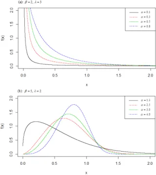
The graphical representation of the density function of TPGLD for some fixed value of the parameters is shown in Figure 1.
236
Figure 1 –Density function of the TPGLD for (a):β=2,λ=3; (b):β=5,λ=2.
TABLE 1
Distributions and corresponding G(x;φ).
Distributions Density function G(x;φ) Authors
Lindley θ2(1(+1+xθ)e)−θx x Lindley (1958)
Power Lindley αθ2(1+x(1α+)xθα)−1e−θxα xα Ghitanyet al.(2013)
Sushila θ2(1(+1+xθ)e)−θx βx Shankeret al.(2013)
Lindley-Pareto βθ2eθx2β−1e−[θ(
x α)β]
α2β(1+θ) (
x
θ)β−1 Lazri and Zeghdoudi (2016)
Lindley-Half Logistic θ2(1+ex)e[
θ
2(1−e x)+x]
[4(1+θ)] e
x−1
2 Silvaet al.(2017)
3. SURVIVAL AND HAZARD RATE FUNCTION
LetX be a continuous random variable with density function f(x)and cumulative dis-tribution functionF(x). The survival (reliability) function and hazard rate (failure rate) function of the three parameter generalized Lindley distribution are defined by
s(x) =(1+λβ+λx α)e−λxα
1+λβ , x>0,θ,λ,β >0, (12) and
h(x) =αλ
2(β+xα)xα−1
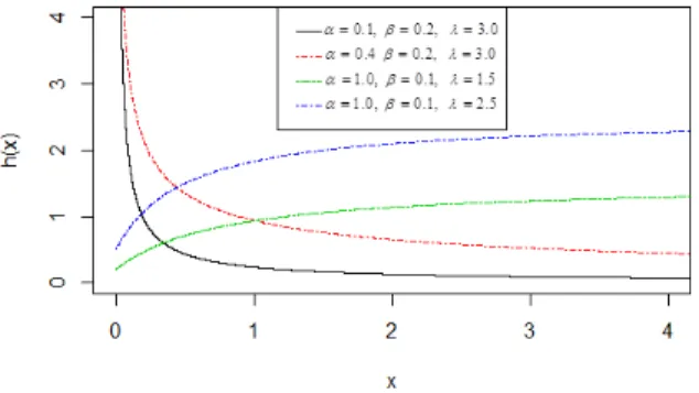
(1+λβ+λxα) , x>0,θ,λ,β >0. (13) The graph of the hazard rate function of the TPGLD for different value of the pa-rameters is given in Figure 2.
Figure 2 –Hazard rate function of the TPGLD.
Clearly from Figure 2, the TPGLD exhibits both monotone increasing and decreas-ing failure rate property. It decreases monotonically whenα <1 and increases mono-tonically whenα≥1.
4. QUANTILES
Given the cumulative distribution functionF(X)defined by Equation (10), the quantile function of the TPGLD can be obtain asQX(p) =F−1(p). The quantile function of the Lindley family of distributions can be expressed in a closed form using the LambertW function proposed in Jodra (2010).
Thepthquantile function is obtained by solvingF(x) = p, i.e.
1−(1+λβ+λx
α)e−λxα
238
(1+λβ+λxα)e−λxα= (1+λβ)(1−p).
Multiplying both sides bye−(1+−λβ), we have
(−1−λβ−λxα)e−(1+λβ+λxα)=−(1+λβ)(1−p)e−(1+λβ).
Clearly, we observe that(−1−λβ−λxα)is the LambertW function of the real argument−(1+λβ)(1−p)e−(1+λβ). Thus, we have
W−1−(1+λβ)(1−p)e−(1+λβ)= (−1−λβ−λxα),
λxα=W−1−(1+λβ)(1−p)e−(1+λβ),
x=
−β−λ1−λ1W−1−(1+λβ)(1−p)e−(1+λβ) 1α
, (14)
where pε(0, 1).
The median of the TPGLD can be obtained by substitutingp= 12in Equation (14) which yields
Median=Q2=
−β− 1 λ−
1 λW−1
−1
2(1+λβ)e
−(1+λβ)
1
α
. (15)
5. MOMENTS
LetX be a continuous random variable with density function f(x), then the rth raw moment ofX is defined by
µ0
r=E(Xr) = Z∞
−∞
xrf(x)d x. (16)
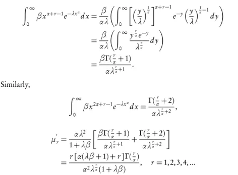
Given the pdf in Equation (11), therthraw moment of the TPGLD is defined by
µ0
r=E(Xr) = Z∞
0
xrαλ2(β+xα)xα−1e−λxα
1+λβ d x
= αλ2
1+λβ
Z ∞
0
βxα+r−1e−λxαd x+ Z∞
0
βx2α+r−1e−λxαd x
.
Using the transformations y=λxα, x= y λ
1α
, d x= 1
αλ y λ
Z∞
0
βxα+r−1e−λxαd x= β
αλ
Z∞
0
y
λ
1αα+r−1 e−yy
λ
1α−1 d y = β αλ Z∞ 0
yαre−y
λr α
d y
=βΓ( r α+1)
αλr α+1
.
Similarly,
Z∞
0
βx2α+r−1e−λxαd x=Γ( r α+2)
αλr α+2
,
µ0
r=
αλ2 1+λβ
βΓ(r α+1)
αλr
α+1 +
Γ(r α+2)
αλr α+2
= r[α(λβ+1) +r]Γ( r α)
α2λαr(1+λβ)
, r=1, 2, 3, 4, ...
(17)
From Equation (17), the first four raw moments of the TPGLD can be obtained as follows
µ0 1=µ=
[α(λβ+1) +1]Γ(1α) α2λ1α(1+λβ)
, µ02=2[α(λβ+1) +2]Γ( 2
α)
α2λ2α(1+λβ)
,
µ0 3=
3[α(λβ+1) +3]Γ(3
α)
α2λα3(1+λβ)
, µ04=4[α(λβ+1) +4]Γ( 4
α)
α2λ4α(1+λβ)
,
so that the variance (σ2), coefficient of variation (γ), measure of skewness (Sk) and mea-sure of kurtosis (Ks) of the TPGLD can be obtained as
σ2= µ0
2−µ2, γ= σ
µ, Sk=
µ0 3−3µ
0
2µ+2µ3 µ0
2−µ2
32
and
Ks = µ
0 4−4µ
0 3µ+6µ
0
2µ2−3µ4 µ0
2−µ2
2 .
240
TABLE 2
Theoretical moments of TPGLD for selected values of the parameters.
α β λ µ0
1 µ 0 2 µ 0 3 µ 0
4 σ2 γ Sk Ks
2 2 3 0.5482 0.3810 0.3107 0.2857 0.0804 2.0070 0.5981 3.1661
4 0.4677 0.2778 0.1939 0.1528 0.0590 2.3523 0.6097 3.1919
3 3 0.5372 0.3667 0.2942 0.2667 0.0780 2.0479 0.6134 3.2003 4 0.4602 0.2692 0.1853 0.1442 0.0575 2.3910 0.6201 3.2164
4 2 3 0.7133 0.5482 0.4464 0.3810 0.0394 1.5424 -0.1105 2.7428 4 0.6587 0.4677 0.3520 0.2778 0.0338 1.6703 -0.1020 2.7434
3 3 0.7059 0.5372 0.4334 0.3667 0.0389 1.5586 -0.0994 2.7438 4 0.6532 0.4602 0.3437 0.2692 0.0334 1.6843 -0.0947 2.7449
6. RENYI ENTROPY
An entropy of a random variableX is a measure of variation of uncertainty associated with the random variableX. Renyi (1961) defined the Renyi entropy ofX with density functionf(x)as
τR(γ) =
1 1−γlog
Z
fγ(x)d x
, γ >0,γ6=1. (18)
Using Equation (18), the Renyi entropy of the TPGLD is defined by
τR(γ) =
1 1−γ log
Z∞
0
(αλ2)γ(β+xα)γxγ(α−1)e−γλxα
(1+λβ)γ d x
= 1
1−γ log
αλ2 1+λβ
γZ∞
0
(β+xα)γxαγ−γe−γλxαd x
.
(19)
From the series expansion
(a+b)n= ∞ X
j=0
n
j
an−jbj,
= 1
1−γlog
αλ2
1+λβ
γ ∞ X
j=0
n
j
βγ−jZ∞
0
xαj+αγ−γe−γλxαd x
,
but
Z∞
0
xαj+αγ−γe−γλxαd x=Γ
j+γ−γα+1
α
α(γλ)j+γ−γ α+α1
so that
τR(γ) =
1 1−γlog
αλ2
1+λβ
γ ∞ X
j=0
n
j
βγ−jΓ
j+γ−γα+α1 α(γλ)j+γ−γα+1
α
= 1
1−γlog
αγ−1λγ(1+1
α)−1α
(1+λβ)γγγ(1−α1)+1α
! ∞ X
j=0
γ j
βγ−j (γλ)jΓ
j+γ−γ α+ 1 α . (20)
7. THE DISTRIBUTION OF THE ORDERED STATISTICS
Suppose thatY1:n<Y2:n<· · ·<Yn:nis the order statistics of a random sample generated from TPGLD, then the probability density function of thekthorder statistics, sayX = Yn:nis given by
gk(x) = n!
(n−k)!(k−1)![G(x)]
k−1[1−G(x)]n−kg(x), (21)
where
g(x) = αλ 2
(1+λβ)(β+x
α)xα−1e−λxα
, G(x) =1−(1+λβ+λx
α) (1+λβ) e
−λxα
,
gk(x) = n! (n−k)!(k−1)!
∞ X
j=0
n
−k j
(−1)j[G(x)]j+k−1g(x)
gk(x) = αλ 2n!
(n−k)!(k−1)!(1+λβ) ∞ X
j=0
n
−k j
(−1)j(β+xα)xα−1e−λxα
×
1−(1+λβ+λx
α) (1+λβ) e
−λxαj+k−1
.
(22)
Using the series expression
1−(1+λβ+λx
α) (1+λβ) e−λx
αj+k−1
=X∞ m=0
j+k
−1 m
(−1)m(1+λβ+λx
α) (1+λβ)m e
−mλxα
,
Equation (22) becomes
= αλ2+pβp+1−qn! (n−k)!(k−1)!(1+λβ)m+1
∞ X
j=0
j X
m=0
m X
p=0
p+1
X
q=0
n
−k j
j+k
−1 m
m
p
×
p+1 q
(−1)j+mxα(1+q)−1e−λ(m+1)xα.
242
Thesthmoment of thekthorder statistics from the TPGLD is defined by
E(Xks) = Z∞
0
xsgk(x)d x (24)
= αλ2+pβp+1−qn! (n−k)!(k−1)!(1+λβ)m+1
∞ X
j=0
j X
m=0
m X
p=0
p+1
X
q=0
n
−k j
j+k
−1 m
m
p
×
p+1 q
(−1)j+m
Z∞
0
xs+α(1+q)−1e−λ(m+1)xαd x
(25)
but
Z∞
0
xs+α(1+q)−1e−λ(m+1)xαd x = Γ s
α+q+1
α(λ(m+1))sα+q+1
.
Thus
E(Xks) = αλ
2+pβp+1−qn! (n−k)!(k−1)!(1+λβ)m+1
∞ X
j=0
j X
m=0
m X
p=0
p+1
X
q=0
n
−k j
j+k
−1 m × m p
p+1 q
(−1)j+m Γ s
α+q+1
α(λ(m+1))αs+q+1
.
(26)
8. MAXIMUM LIKELIHOOD ESTIMATION
Let(x1,x2,· · ·,xn)be random samples from the TPGLD, then the log-likelihood func-tion is defined as
`(x,φ) =
n X
i=1 log
αλ2(β+
xα)xα−1e−λxα
1+λβ
, φ= (α,β,λ)T, (27)
=nlogα+2nlogλ+
n X
i=1
log(β+xiα)+(α−1)
n X
i=1
logxi−λ n X
i=1
(xiα)−nlog(1+λβ). (28)
∂ ` ∂ α =
n
α+
n X
i=1
xiαlogxi (β+xiα)+
n X
i=1
logxi−λ
n X
i=1
xiαlogxi, ∂ `
∂ λ = 2n
λ −
n X
i=1
xαi − nβ
(1+λβ).
The maximum likelihood estimator ˆφofφcan be obtained by solving the system of non-linear equation ∂ φ∂ ` =0. This non-linear equation can be solved using the Newton Raphson iterative scheme given by
ˆ
φ = φk−H−1(φk)U(φk), (29)
whereU(φk)is the score function andH(φk)is the Hessian matrix, which is the second derivative of the log-likelihood function.
A closed form expression of the Fisher information matrix is defined by
I(φk) =−E[H(φk)] =−E
∂2`
∂ α2
∂2`
∂ α∂ β ∂
2`
∂ α∂ λ
∂2`
∂ β∂ α ∂
2`
∂ β2
∂2`
∂ β∂ λ
∂2`
∂ λ∂ α ∂
2`
∂ λ∂ β ∂
2`
∂ λ2
The elements of the observed information matrix of the TPGLD are available upon request from the authors.
9. DATA ANALYSIS
In this section, we fit the proposed distribution to two real data sets alongside with some well-known lifetime distributions with the following density functions.
(i) Exponentiated Power Lindley distribution (EPLD) reported in Warahena-Liyanage and Pararai (2014):
f(x) =αλ
2β(1+xα)xα−1e−λxα
1+λ
1−
1+ λxα 1+λ
e−λxα
β−1
, x>0,α,λ,β >0.
(ii) Exponentiated Lindley geometric distribution (ELGD) reported in Wang (2013):
f(x) =αβ
2(1−λ)(1+x)e−βx
1−1+1βx+βe−βxα−1 (1+β)1−λ+λ
1−1+1βx+βe−βxα2
244
(iii) Power Lindley distribution (PLD) reported in Ghitanyet al.(2013):
f(x) = αλ2(1+xα)xα−1e−λx
α
1+λ , x>0,α,λ >0.
(iv) Lindley-exponential distribution (LED) reported in Bhatiet al.(2015):
f(x) = αλ
2e−αx(1−e−αx)λ−1(1−l o g(1−e−αx))
1+λ , x>0,α,λ >0.
(v) Lindley distribution reported in Lindley (1958):
f(x) =λ
2(1+x)e−λ
1+λ , x>0,λ >0.
The comparison criteria considered in this work includes, the estimates of the param-eters of the distribution,−2 log(L), Akaike information criterion[AI C=2k−2 log(L)], Bayesian information criterion [B I C = klog(n)−2 log(L)], Anderson Darling test statistic(A∗)and Crammer-von Mises test statistic(W∗), wherenis the number of
ob-servations,kis the number of estimated parameters andLis the value of the likelihood function evaluated at the parameter estimates.
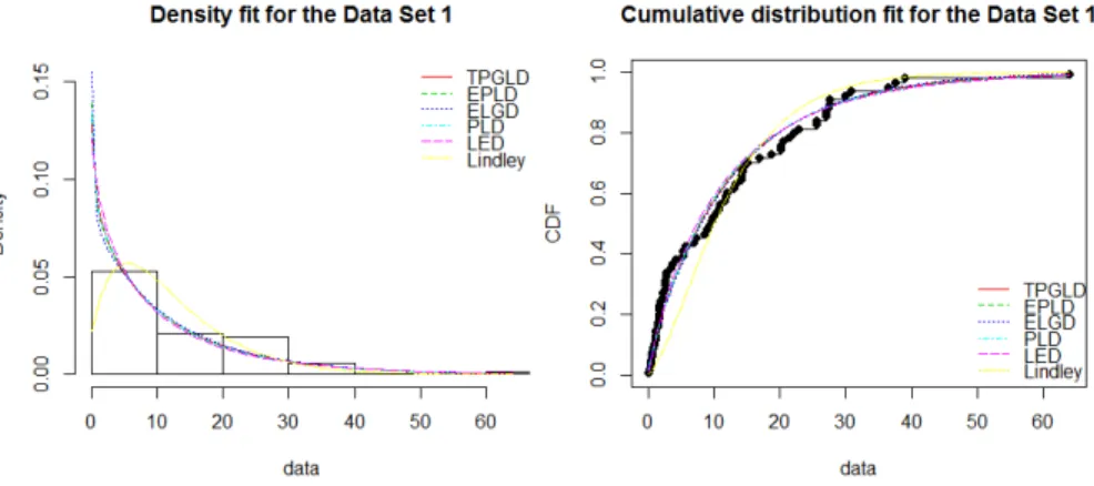
Data Set 1:This data set consists of 72 exceedances of flood peaks (inm3/s) of the Wheaton river near Carcross in Yukon Territory, Canada for the years 1958-1984. This data was first used by Choulakian and Stephens (2001) to examine the applicability of the generalized Pareto distribution and also was reported in Akinseteet al.(2008). This data set is given in Table 3.
TABLE 3
Exceedances of Wheaton river flood data.
1.7 2.2 14.4 1.1 0.4 20.6 5.3 0.7 1.9 13.0 12.0 9.3 1.4 18.7 8.5 25.5 11.6 14.1 22.1 1.1 2.5 27.0 14.4 1.7 37.6 0.6 2.2 39.0 0.3 15.0 11.0 7.3 22.9 1.7 0.1 1.1 0.6 9.0 1.7 7.0 20.1 0.4 2.8 14.1 9.9 10.4 10.7 30.0 3.6 5.6 30.8 13.3 4.2 25.5 3.4 11.9 21.5 27.6 36.4 2.7 64.0 1.5 2.5 27.4 1.0 27.1 20.2 16.8 5.3 9.7 27.5 2.5
Plots of the density and the cumulative distribution fit for the Wheaton river flood data is shown in Figure 3.
TABLE 4
Summary statistics for the data set 1 (standard error in parenthesis).
Models Estimates -2 log L AIC BIC A∗ W∗
TPGLD α=0.870(0.110)
β=16.515(35.714) 502.730 508.730 515.560 0.808 0.141 λ=0.154(0.083)
EPLD α=0.730(0.236)
β=0.916(0.599) 504.425 510.425 517.255 0.858 0.149 λ=0.300(0.281)
ELGD α=0.559(0.121)
β=0.095(0.024) 505.089 511.089 517.919 0.842 0.141 λ=0.281(0.466)
PLD α=0.700(0.057) 504.444 508.444 512.997 0.877 0.153 λ=0.339(0.056)
LED α=0.062(0.012) 503.073 507.073 511.626 0.845 0.154 λ=1.121(0.141)
Lindley α=0.150(0.013) 528.424 530.424 532.700 7.421 0.818
246
TABLE 5 Strength of glass fibers data.
0.55 0.93 1.25 1.36 1.49 1.52 1.58 1.61 1.64 1.68 1.73 1.81 2.00 0.74 1.04 1.27 1.39 1.49 1.53 1.59 1.61 1.66 1.68 1.76 1.82 2.01 0.77 1.11 1.28 1.42 1.50 1.54 1.60 1.62 1.66 1.69 1.76 1.84 2.24 0.81 1.13 1.29 1.48 1.50 1.55 1.61 1.62 1.66 1.70 1.77 1.84 0.84 1.24 1.30 1.48 1.51 1.55 1.61 1.63 1.67 1.70 1.78 1.89
TABLE 6
Summary statistics for the data set 2 (standard error in parenthesis).
Models Estimates -2 log L AIC BIC A∗ W∗
TPGLD α=4.944(0.658)
β=3.429(4.401) 28.421 34.421 40.851 0.999 0.166 λ=0.156(0.071)
EGLD α=9.521(20.587)
β=6.217(0.628) 31.663 37.663 44.093 1.280 0.171 λ=-653.220(1341.380)
PLD α=4.458(0.387) 29.380 33.380 37.666 1.119 0.190 λ=0.222(0.047)
LED α=2.612(0.239) 62.816 66.816 71.102 4.341 0.799 λ=32.308(9.558)
Lindley α=0.996(0.095) 162.557 164.557 166.700 16.245 3.332
Plots of the density and the cumulative distribution fit for the strengths of glass fiber data are shown in Figure 4. When comparing lifetime distributions, the distribution with the smallest−2 logL, AIC, BIC,A∗andW∗is considered to be the best model in
fitting a given data set. However, when the number of parameters of a distribution is small, the likelihood of selecting such a distribution as the best model will be increased in terms of−2 logL, AIC and BIC. In this case, one resort to measures of goodness of fit test statistics such as Anderson Darling test, Crammer-von Mises test and Komolgorov-Smirnov test statistics to validate the superiority of a model for a given data set. Conse-quently, Tables 4 and 6 show that the TPGLD has the least value of−2 logL, AIC, BIC, A∗andW∗, which indicates that the TPGLD demonstrates superiority over the EPLD,
ELGD, PLD, LED and the classical one parameter Lindley distribution in modeling the lifetime data sets under study. This claim was further supported by inspecting the density and cumulative distribution fit of the distributions for the real lifetime data set.
REFERENCES
A. AL-BABTAIN, A. M. EID, A. N. AHMED, F. MEROVCI(2015).The five parameter Lindley distribution. Pakistan Journal of Statistics, 31, no. 4, pp. 363-384.
A. ALZAARTREH, C. LEE, F. FAMOYE(2013).A new method for generating families of continuous distributions. Metron, 71, no. 1, pp. 63-79.
A. AKINSETE, F. FAMOYE, C. LEE(2008).The beta-Pareto distribution. Statistics, 42, pp. 547-563.
H. BAKOUCH, B. AL-ZAHRANI, A. AL-SHOMRANI, V. MARCHI, F. LOUZAD (2012).
An extended Lindley distribution. Journal of the Korean Statistical Society, 41, pp. 75-85.
W. T. BERA (2015).The Kumaraswamy Inverse Weibull Poisson Distribution with Ap-plications. Theses and Dissertations, 1287. Indiana University of Pennsylvania. http://knowledge.library.iup.edu/etd/1287
D. BHATI, M. A. MALIK, H. J. VAMAN(2015).Lindley-exponential distribution: Prop-erties and applications. Metron, 73, no. 3, pp. 335-357.
V. CHOULAKIAN, M. A. STEPHENS(2001). Goodness-of-fit for the generalized Pareto distribution. Technometrics, 43, no.4, pp. 478-484.
M. GHITANY, B. ATIEH, S. NADADRAJAH(2008).Lindley distribution and its applica-tions. Mathematics and Computers in Simulation, 78, pp. 493-506.
M. GHITANY, D. AL-MUTAIRI, N. BALAKRISHNAN, I. AL-ENEZI(2013).Power
248
P. JODRA (2010). Computer generation of random variables with Lindley or Pois-son–Lindley distribution via the Lambert W function. Mathematical Computations and Simulation, 81, pp. 851-859.
N. LAZRI, H. ZEGHDOUDI(2016).On Lindley-Pareto Distribution: Properties and Ap-plication. Journal of Mathematics, Statistics and Operations Research, 3, no.2, pp. 1-7.
D. V. LINDLEY(1958).Fiducial distributions and Bayes’ theorem. Journal of the Royal Statistical Society, Series B, 20, no. 1, pp. 102-107.
R. MAYA, M. R. IRSHAD(2017).New extended generalized Lindley distribution:
Proper-ties and applications. Statistica, 77, no. 1, pp. 33-52.
S. NADARAJAH, H. BAKOUCH, R. TAHMASBI(2011).A generalized Lindley distribu-tion. Sankhya B: Applied and Interdisciplinary Statistics, 73, pp. 331-359.
A. RÉNYI(1961).On measure of entropy and information. Proceedings of the 4th Berke-ley Symposium on Mathematical Statistics and Probability, University of California Press, Berkeley, pp. 547-561.
R. SHANKER, S. SHARMA, U. SHANKER, R. SHANKER(2013).Sushila distribution and its application to waiting times data. International Journal of Business Management, 3, no. 2, pp. 1-11.
F. G. SILVA, A. PERCONTINI, E. BRITO, M. V. RAMOS, R. VENANCIO, G. CORDEIRO (2017). The odd Lindley-G family of distributions. Austrian Journal of Statistics, 46, pp. 65-87.
R. L. SMITH, J. NAYLOR (1987).A comparison of maximum likelihood and Bayesian
estimators for the three-parameter Weibull distribution. Applied Statistics, pp. 358-369. G. WARAHENA-LIYANAGE, M. PERARAI(2014).A Generalized Power Lindley Distri-bution with Applications. Asian Journal of Mathematics and Applications (article ID ama0169), pp. 1-23.
SUMMARY
In this paper, we introduced a new class of lifetime distribution and considered the mathemati-cal properties of one of the sub models mathemati-called a three parameter generalized Lindley distribution (TPGLD). The new class of distributions generalizes some of the Lindley family of distribution such as the power Lindley distribution, the Sushila distribution, the Lindley-Pareto distribution, the Lindley-half logistic distribution and the classical Lindley distribution. An application of the TPGLD to two real lifetime data sets reveals its superiority over the exponentiated power Lindley distribution, the exponentiated Lindley geometric distribution, the power Lindley distribution, the Lindley-exponential distribution and the classical one parameter Lindley distribution in mod-eling the lifetime data sets under study.