Simultaneous Feedback Models with Macro-Comparative Cross-Sectional Data

Simultaneous Feedback Models with

Macro-Comparative Cross-Sectional Data

Nate Breznau

Mannheim Centre for European Social Research (MZES)

Abstract

Social scientists often work with theories of reciprocal causality. Sometimes theories sug-gest that reciprocal causes work simultaneously, or work on a time-scale small enough to make them appear simultaneous. Researchers may employ simultaneous feedback mod-els to investigate such theories, although the practice is rare in cross-sectional survey re-search. This paper discusses the certain conditions that make these models possible if not desirable using such data. This methodological excursus covers the construction of simul-taneous feedback models using a structural equation modeling perspective. This allows the researcher to test if a simultaneous feedback theory fits survey data, test competing hypotheses and engage in macro-comparisons. This paper presents methods in a manner and language amenable to the practicing social scientist who is not a statistician or matrix mathematician. It demonstrates how to run models using three popular software programs (MPlus, Stata and R), and an empirical example using International Social Survey Pro-gram data.

Keywords: simultaneous feedback model, cross-sectional data, macro-comparative research, structural equation modeling, reciprocal causality, Mplus, Stata, R (lavaan)

Acknowledgments

I am grateful to two anonymous reviewers, discussions on SEMNET, Bart Meuleman and Sebastian Pink for helpful instruction and comments.

Direct correspondence to

Nate Breznau, Mannheim Centre for European Social Research (MZES) E-Mail: [email protected]

Social scientists often study reciprocally causal phenomena. For example, sup-ply and demand in economics; candidate evaluations and party identification in political science; road investment and travel demand in geography; and educational attainment and parenthood entry in sociology and demography (Marini, 1984; Page & Jones, 1979; Xie & Levinson, 2010). When timings of reciprocal causes are unobservable or occur contemporaneously, a state of simultaneous feedback exists. Rather than in cycles, events happen at the same time. Philosophers of causality question the existence of simultaneous feedback (Mulaik, 2009: Chapter 3); how-ever, researchers regularly face theoretical and data conditions that force them to accept simultaneous feedback in practice. This is particularly acute in macro-com-parative survey research where observations take place over a year, but theoretical causes may take place at less-than-yearly intervals. All sub-yearly causal effects appear simultaneous within a year interval. Under certain conditions, macro-com-parative researchers can employ simultaneous feedback models (SFMs) to capture these effects, allowing them to overcome some limitations of comparative cross-sectional survey research.

Herein, I elaborate when and how to use SFMs. This requires structural equa-tion modeling (SEM) strategies to explicate theoretical relaequa-tionships before extract-ing meanextract-ingful statistical results. I use minimal statistical and mathematical

jar-gon without matrix algebra1_{, and a practical example of public opinion and social}

policy. I show that SFMs provide a powerful method for macro-comparative survey researchers to explain, predict and compare reciprocally causal phenomena.

Simultaneous Feedback

Instances where two phenomena are co-causes of each other are ubiquitous in social

research2_{; however, modeling reciprocal causality is challenging. Time is usually}

1 Matrix algebra is the basis of nearly all social science statistics including SFMs; how-ever, this excursus is for the practicing social scientist who is unlikely a matrix alge-braician.

the basis for explaining or predicting things (Elwert, 2013; Pedhazur, 1997). To be a cause or a useful predictor, X must take place prior to Y. If X happened after Y it

is not a cause3_{. Sometimes researchers cannot effectively observe or}

operational-ize time. For example, the moods of roommates are theoretically timed causes of each other but may unfold so quickly that they appear simultaneously causal (Sie-gel & Alloy, 1990). It is possible that there are nanoseconds in between, but these are unobservable. Furthermore, excessive complexity of timings and multitudinous mood causes running in both directions leave the researcher viewing mood effects as simultaneous.

Macro-comparative research is similar on a larger time scale. Contextual data tend to measure time points spanning an entire year. Reciprocally causal effects that take place in just days, weeks or even months subsume into these yearly obser-vations. For example, public opinion likely causes changes in policymaking on a weekly or monthly basis as policymakers constantly try to meet public preferences. Simultaneously, public opinion changes within minutes or hours in response to policy changes. When capturing these opinion-policy effects with survey data, the two appear to have simultaneous causality within each year unit. Moreover, survey researchers lack yearly comparative opinion data across countries, e.g.,

cross-sec-tional yearly time-series4_{, rendering longitudinal methods sometimes}

inappropri-ate. Having sporadic macro-comparative survey data means SFMs might be appro-priate, but this is not a sufficient condition to use them. Theory must drive this decision (Hayduk et al., 2007; Kaplan, Harik, & Hotchkiss, 2001).

Given a theory of simultaneous feedback between two phenomena, I label

them Y1 and Y25, where at least two different linkages exist between them if not

more. One for the effect of Y₁ on Y₂ and one vice-versa. However, when I observe

and quantify Y1 and Y2 as variables, they have only one empirical linkage: their

covariance (or correlation). Identifying two effects statistically, when there is only

one covariance, is not possible. Y1 and Y2 are nonrecursive meaning that their

respective effects on each other cannot be identified using only their joint informa-tion. Their reciprocal relationship makes them endogenous meaning caused from

3 The method herein applies to causal or explanatory research subsuming causes or sev-eral causes into a package of predictive power without considering the mechanisms in detail. Although causality is at the heart of the theoretical side of SFMs, the vast realm of mathematics and philosophy of causality is beyond the scope of this paper (Pearl, 2010; Sobel, 1996).

4 Although impressive, many macro-comparative sources of survey data barely qualify as longitudinal, cross-sectional time-series when fielded only every 2 to 10 years (e.g., European Social Survey, World Values Survey and International Social Survey Pro-gram).

5 I use Y1 and Y2 rather than X and Y, because Y denotes dependent variables.

within; however, identifying these nonrecursive endogenous effects requires some exogenous causes from without.

I describe this problem using Equations 1 and 2, and Figure 1. Both cases present a system logically underidentified – there are more parameters to be

esti-mated than pieces of observed information (two coefficients b₁ and b₂ yet only one

covariance of Y1 and Y2).

1 1 2 1

Y b Y e= + (1)

2 2 1 2

Y =b Y e+ (2)

Regression analysis could estimate Equations 1 and 2, but results are probably inaccurate given a theory of reciprocal causality. In Figure 1 the arrows represent

theoretical effects, and b₁ and b₂ represent regression coefficients. Y₁ is not known

without knowing Y2 and Y2 is not known without knowing Y1: An endless circle!

Identifying b₁ and b₂ is an exercise in finding more variables or parameters.

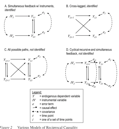
Figure 2 gives four common formal models containing reciprocal causality, some identified, others not. Adding instrumental variables (IVs) enables identification of

unique b1 and b2 effects. An IV is exogenous: not caused by the system described

in the model, not caused by Y₁ or Y₂ and not moderating or somehow causing the

causal paths linking Y1 and Y2. Figure 2A describes some phenomenon labeled Y1

occurring at time “t” that is both a cause (arrow pointing away) and outcome (arrow

pointing towards) of another phenomenon Y2 measured at the same time. In this,

IV₁ must be a cause of Y₁ but not of Y₂; and IV₂ must cause Y₂ but not Y₁ (see section

“Instrumental variables”).

Figure 2A is the basic SFM form.

Other common reciprocal effects models appear in Figure 2B-2D. Cross-lagged reciprocal effects (2B) are a common form of reciprocal causal modeling

(for discussions: Billings & Wroten, 1978; Schaubroeck, 1990). Looking at Y1 and

Y₂ longitudinally over time generates separate, unique covariances between Y₁

and Y2; one for Y2,t-1 with Y1,t and another for Y1,t-1 with Y2,t. Cross-lagged models

require the assumption that Y₁ and Y₂ do not cause each other simultaneously for

identification (omitted arrows between them at time t). Macro-comparative survey researchers rarely have sequential time series of survey data in several countries making these models untenable, often because of missing time points or the exact

4

Figure 1. Path Model of Equations 1 and 2

b2

𝑌𝑌1 𝑌𝑌2

In Figure 1 the arrows represent theoretical effects, and 𝑏𝑏1 and 𝑏𝑏2 represent regression coefficients.

Identifying 𝑏𝑏1 and 𝑏𝑏2 is an exercise in finding more variables or parameters. Figure 2 gives

four models of 𝑌𝑌1 and 𝑌𝑌2 that are common formal models containing reciprocal causality, some

identified, others not. Adding instrumental variables (𝐼𝐼𝐼𝐼s) enables identification of unique 𝑏𝑏1 and 𝑏𝑏2

effects. An 𝐼𝐼𝐼𝐼 is exogenous: not caused by the system described in the model, not caused by 𝑌𝑌1 or 𝑌𝑌2

and not moderating or somehow causing the causal paths linking 𝑌𝑌1 and 𝑌𝑌2. Figure 2A describes

some phenomenon labeled 𝑌𝑌1 occurring at time “t” that is both a cause (arrow pointing away) and

outcome (arrow pointing towards) of another phenomenon 𝑌𝑌2 measured at the same time. In this, 𝐼𝐼𝐼𝐼1

must be a cause of 𝑌𝑌1 but not of 𝑌𝑌2; and 𝐼𝐼𝐼𝐼2 must cause 𝑌𝑌2 but not 𝑌𝑌1 (see section “Instrumental

variables”).

Figure 2A is the basic SFM form.

b1

e2

e1

b2

timing of cause and effect do not match the starting and ending points of the survey (Finkel, 1995). If causes occur at a less-than-yearly interval, in addition to across time-units, then Figure 2C is accurate visually but underidentified statistically. A similar story occurs when adding instrumental variables to 2C as shown in 2D. The instruments do not add enough power to overcome the cyclically recursive problem

of observing Y1 and Y2 over time because they are causes of their later selves in

addition to causing each other leading again to too many parameters.

5

Figure 2. Various Models of Reciprocal Causality

Other common reciprocal effects models appear in Figure 2B-2D. Cross-lagged reciprocal effects (2B) are a common form of reciprocal causal modeling (for discussions: Billings & Wroten, 1978; Schaubroeck, 1990). Looking at 𝑌𝑌1 and 𝑌𝑌2 longitudinally over time generates separate, unique covariances between 𝑌𝑌1 and 𝑌𝑌2; one for 𝑌𝑌2,𝑡𝑡−1 with 𝑌𝑌1,𝑡𝑡 and another for 𝑌𝑌1,𝑡𝑡−1 with 𝑌𝑌2,𝑡𝑡. Cross-lagged models require the assumption that 𝑌𝑌1 and 𝑌𝑌2 do not cause each other simultaneously for identification (omitted arrows between them at time t). Macro-comparative survey researchers do not have sequential time series of survey data in several countries making these models untenable, often because of missing time points or the exact timing of cause and effect do not match the starting and ending points of the survey (Finkel, 1995). If causes occur at a less than yearly interval, in addition to across time-units, then Figure 2C is accurate visually but underidentified statistically. A similar story occurs when adding instrumental variables to 2C as shown in 2D. The instruments do not add enough power to overcome the cyclically recursive problem of observing 𝑌𝑌1 and 𝑌𝑌2 over time

Y2,t-1 Y2,t

Y1,t

Y1,t-1

IV2 Y2,t

Y1,t IV1

Y2,t-1 Y2,t

Y1,t

Y1,t-1

e1

e2

C. All possible paths, not identified

B. Cross-lagged, identified

e1

e2 e1

e2

A. Simultaneous feedback w/ instruments,

identified

Legend:

Y = endogenous dependent variable

IV = instrumental variable

e = error term

= causal effect = covariance

t = time point

i = one of a set of time points

Y2,t-i Y2,t

Y1,t

Y1,t-i

e1

e2

D. Cyclical recursive and simultaneous feedback, not identified

IV2

IV1

e2i

e1i

Conditions Necessary for Simultaneous Feedback

Models

A strong theory, equilibrium, model identification and appropriate instrumental variables are the necessary features to employ Figure 2A.

Theory

The first and most important requirements of SFMs are theoretical. Without

the-ory, the two arrows connecting Y1 and Y2 do not exist. There must be an a priori

logic to the data-generating model, defensible against confounding effects (Heck-man, 2000; Rigdon, 1995). Thus, a theory of simultaneous causality is the baseline condition. This theory must specify that during the observational window causal

effects materialized between Y1 and Y2; regardless of whether these are direct or

operating through intermediary mechanisms. A researcher must provide sufficient argument for simultaneity. That of, (1) co-determinacy with effects that happen ‘instantaneously’ in less time than can be observed, or (2) complexity with effects that are constantly taking place going in many directions having various lengths of time to complete; so as to appear simultaneous. Without this theoretical basis

to the Y1 and Y2 relationship, researchers have no ground to stand on in defense of

simultaneous feedback (Hayduk et al., 2007; Markus, 2010). Theory determines the design of a formal path model, instrumental variables, equilibrium, size and direction of effects, the set of independent variables, and the nature of errors and estimation techniques. Suffice to say, theory is paramount.

Equilibrium

Two forms of equilibrium need be present in SFMs. The first is that causal effects are theoretically stable or behave in a stable manner. There should be logical

argu-ment that the impact of Y1 on Y2 and vice-versa, do not change over time (Kaplan

et al., 2001). In other words, the effects should not depend on when in time the

researcher observes Y1 and Y2 (Sobel, 1990). This is a grey area as inevitably all

before and after. If the model includes events before and after this change, it is mis-specified as a SFM.

The second part is that the causal effects are part of a context at equilibrium, e.g., a political or judicial system. If a system experiences shocks then equilibrium is unlikely, e.g., disruptive wars or economic recessions. Therefore, the researcher

must rule out changes to the larger systems within which Y1 and Y2 operate (see

sec-tion “Disequilibrium”).

Identification

Any formal model, including one with simultaneous feedback must be identified to

produce meaningful results or results at all6_{. To identify two statistical coefficients}

that capture two theoretical effects between Y1 and Y2 there must be more than one

covariance in the model. Only one covariance in the feedback model is underi-dentified, meaning more parameters to estimate than pieces of observed informa-tion leading to a negative value for model degrees of freedom. Pieces of observed information are all parameters the researcher observes in the data including the means, variances and covariances of the variables in the model, also known as model “elements” (Rigdon, 1994). In SFMs, the observed means are often not

esti-mated because researchers’ main interests are in the coefficients between Y1 and Y2

that derive entirely from covariances, irrespective of means. Adding means to the analysis generally complicates things with few cases.

Without means, the formula to calculate pieces of observed model

informa-tion is v v

( )

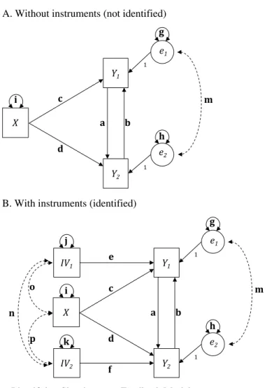
model needs a minimum of the same number of model elements as freely estimated parameters for identification, i.e., model degrees of freedom needs to be larger than or equal to zero. To illustrate, I add one predictor variable X, as shown in Figure

3. Figure 3A is not identified because it requires estimation of four coefficients (a

through d) and three variances (g through i), with residual covariance m optional.

Fixing m to zero for now, and knowing nothing about a through i, there are seven

freely estimated parameters (a through i). That means I need seven pieces of

infor-mation for a just-identified model. There are only six pieces in Figure 3A: three

covariances (X,Y1| , | ,X Y Y2 1 Y2) and three variances (for X Y Y, 1& 2), or 3(4)/2=6.

Thus, model degrees of freedom is smaller than zero (six minus seven). Figure 3A is underidentified.

Figure 3B includes IV1 and IV2, creating 5(6)/2 = 15 pieces of information.

Assuming that the IVs and the error terms are correlated (parameters n and m

respectively), the model has 15 freely estimated parameters (all letters in 3B),

meaning model degrees of freedom is zero and the model is just-identified. An ideal model has more than zero, for example three IVs leads to 6(7)/2=21 pieces of observed information and 20 freely estimated parameters; degrees of model free-dom equals one. However, IVs are difficult to find. An identification rule requires

at least one IV for each Y variable. If both instruments are attached to Y₂, and none

to Y1, the model might have degrees of freedom greater than zero, but the model is

still not identified without an IV for Y₁. This is known as the rank condition. This

condition is satisfied when, “each variable in a feedback loop has a unique pattern of direct effects on it from variables outside the loop” (Kline, 2011, p. 135). Adding

8

Figure 3. Identifying Simultaneous Feedback Models

B. With instruments (identified)

Figure 3B includes

𝐼𝐼𝐼𝐼

and

𝐼𝐼𝐼𝐼

, creating 5(6)/2 = 15 pieces of information. Assuming that the

𝐼𝐼𝐼𝐼

s and the error terms are correlated (parameters

n

and

m

respectively), the model has 15 freely

estimated parameters (all letters in 3B), meaning model degrees of freedom is zero and the model is

just-identified. An ideal model has more, for example three

𝐼𝐼𝐼𝐼

s leads to 6(7)/2=21 pieces of

observed information and 20 freely estimated parameters; degrees of model freedom equals one.

However,

𝐼𝐼𝐼𝐼

s are difficult to find, as I discuss next. An identification rule requires at least one

𝐼𝐼𝐼𝐼

for

each

𝑌𝑌

variable. If both instruments are attached to

𝑌𝑌

, and none to

𝑌𝑌

, the model would lead to

degrees of freedom greater than zero, but the model is still not identified without an

IV

for

𝑌𝑌

. This is

known as the rank condition. This condition is satisfied when, “each variable in a feedback loop has

a unique pattern of direct effects on it from variables outside the loop” (Kline, 2011, p. 135). Adding

more

𝑋𝑋

variables to 3B does not help with identification as it does not change the degrees of model

freedom nor add

unique

direct effects.

1 1

Y2 Y1

e2 e1

X a b

c

d

g

h

i m

e

f

1 1

Y2 Y1

e2 e1

X a b

c

d

g

h

i m

IV1

IV2

k j

n o

p

more X variables to 3B does not help with identification as it does not change the degrees of model freedom nor add unique direct effects.

Instrumental Variables

Identification depends on instrumental variables (IV1 and IV2). Necessary

condi-tions for selecting IVs are theoretical and statistical. “Instrumental variables” is both an estimation technique and a label for specific exogenous variables (Sargan, 1958). This section is devoted to exogenous variables, saying nothing of estimation

techniques7_{. An IV must be exogenous to the dependent variable. In experimental}

language, IV causes the distribution of a treatment but not the outcome. In

non-experimental language, the endogenous variable depends on the values of the IV independently from the dependent variable, or the dependent variable only shows covariance with the IV after conditioning on the endogenous variable.

In Figure 3B, the IV for Y1 must not cause Y2. If IV1 is a cause of Y2 then IV1

is an independent variable, not an IV. All independent variables explain or predict

all endogenous variables, thus are part of the data-generating model of Y2 (and Y1).

For IV1 to pass it must not be part of the data-generating model of Y2. This is the

exclusion restriction. The problem is not correlation of IV1 with Y2, but correlation

of IV₁ with e2; i.e., correlation with the unexplained disturbance or error in the

dependent variable after adjusting for the impact of all independent variables. If IV1

causes Y2, or omitted variables cause both IV1 and Y2 then a correlation of IV1 with

e₂ exists; and the larger this correlation, the larger the problems with the IV. If IV1

has a small correlation with e2 because of measurement or random error, then as

the sample size approaches infinity the correlation approaches its true value of zero

(i.e., asymptotic correlation = 0). If so, small IV1 with Y2 correlations after adjusting

for covariates are acceptable.

When meeting these conditions, IV1 and IV2 decompose the single

correla-tion between Y1 and Y2 in Figure 3B into 3 parts: (1) the part that could result from

a causal effect or a shared omitted causal effect of Y1 on Y2 (covariance left after

removing that predicted by IV2), (2) the same for Y2 on Y1, and (3) the unexplained

remaining covariance of error terms e1 and e2. Although technically optional, Part

(3) is usually modeled, because finding instruments that explain everything about

Y₁ and Y2 with no remainder is unlikely. Moreover, the error term e1 is produced

by a causal effect of Y2 (path b). Yet e2 is a part of Y2 and is therefore by definition

a part of the error term e1, i.e., correlated with its own partial correlation produced

from Y2 being regressed on Y1 (Wong & Law, 1999, p. 73). The same is true for

e₂, and therefore specifying no residual correlation may deny the causally defined

model its own properties. Thus, sometimes a cross-sectional nonrecursive model with correlated errors is the ʻbest availableʼ approximation of cross-lagged recipro-cal effects when they are otherwise underidentified.

Even if theoretically not causal, a large correlation between IV1 and Y2 is a

problem statistically. The larger the correlation the more variance that all

indepen-dent variables must explain in Y2 before IV1 is left uncorrelated with e2. In other

words, the partial correlation of IV₁ and Y₂ takes away variance in IV₁ that is

neces-sary to explain Y1. Thus, the larger this correlation, the greater the disruption of the

researcher’s goal to explain variance in Y₁ independent of Y₂ and all independent

variables. An inverse of this problem occurs when IV1 has an increasingly

closer-to-zero correlation with Y₁ (Bartels, 1991). The smaller the correlation, the less unique

variance of Y1 that can be explained by IV1. These two conditions describe a weak

instrument problem. Theoretical arguments establish exclusion restrictions neces-sary to use instrumental variables; however, statistics help identify potential weak instrument problems.

In SEM, model diagnostics, in particular modification indices provide a simple first line of defense to identify weak instruments (see “Fit testing and diagnostics”). This applies because the structural model (what the researcher draws in a path dia-gram and then prodia-grams into the statistical software) fixes the correlation of each IV with each corresponding e to be zero. The fit and modification indices tell the researcher if these fixed zero correlations are realistic given the data. Alternatively, traditional weak instrument tests come from estimating whether results from the instrumental variable estimator and the OLS estimator are consistent, defined in a number of ways depending on the test (Bollen, 2012; Hahn & Hausman, 2002).

There are a variety of statisticians arguing for statistical methods to identify instrumental variables without theoretical arguments that an IV meets the exclu-sion restriction (see “Other concerns”). Although these methods may asymptoti-cally recover a known causal effect (as shown in simulations), the SFM researcher is searching for causal effects whose existence or size is empirically unknown. If already known, research becomes unnecessary. Moreover, even when the

corre-lation of IV₁ and Y₂ is exactly zero, there is no statistical way to know for sure

that IV₁ and e2 do not correlate due to causal or omitted variable linkages.

Sup-pression or omitted variables can easily produce a statistical relationship of zero, when the actual causal relationship is non-zero (MacKinnon, Krull, & Lockwood,

2000)8_{. Thus, theoretical arguments are necessary to rule out ‘backdoor’ or}

con-founding relationships among variables. Finally, arguments must establish that the

instrument is applicable to all cases in the data. If there are cases where the instru-ment might have a unique causal relationship with the independent variable, so that effects are not monotonic, then this is another form of confounding calling for model re-specification.

Although focused on experimental research, a meta-analysis of instrumen-tal variable estimates in political science suggests that researchers routinely fail to offer theoretical arguments that the IV is: (1) unrelated to unobserved/omitted causes of Y, (2) has no direct (causal) effect on Y, and (3) that the instrument could

plausibly affect all cases (Sovey & Green, 2011)9_{. This neglect has grave}

implica-tions for the trustworthiness of results.

An Application – Opinion and Policy

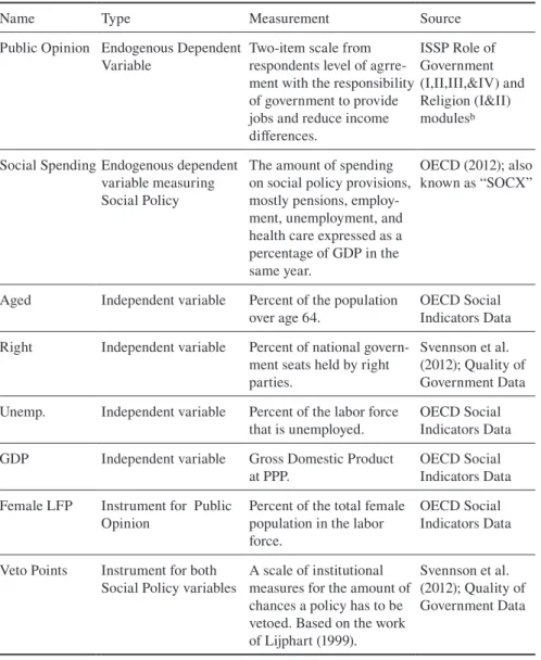
I use the example of Breznau (2017) modeling simultaneous feedback between pub-lic opinion and social spending to provide a didactical picture of SFMs. I only briefly summarize the theory from the original research, to keep the focus on execution of the SFM. Public opinion and social policy are an example of theo-retical simultaneous feedback, because: (1) Opinion and policy are co-determinant occurring at the same moments or overlapping moments in time. Observing public opinion in a one-year unit prevents observation of anything other than simultane-ous effects, even if multiple effects take place within a year. (2) The relationship is so complex that a simultaneous model may come closer to reality than something with arbitrary lags (as taken from years of a survey). Policymakers imagine opinion or act on expected future changes in opinion before opinion changes occur, while public opinion responds to policymakers’ intentions and discussions before they actually change policy. Moreover, opinion responds to many things at once over many points in time and the responses take different lengths to materialize. The same applies to policymaking. Given all these effects starting, maturing, declining and then stopping over time, I expect that there is a simultaneous effect, or average simultaneous effect underlying all effects.

The instruments I employ are female labor force participation (IV1) for public

opinion (Y1) and veto points (IV2) for policy (Y2). Labor force participation

influ-ences policy attitudes. Holding male participation roughly equal (as seen across OECD countries), variation in the distribution of female participation links to changes in aggregate opinion. Women, who are significantly more supportive of social policy than men are, become less supportive when in the labor force, on average. Moreover, the policy ‘styles’ of different countries show no patterning by female labor force participation suggesting that at least in recent decades it has no

effect on social policy in the aggregate (i.e., exogenous from Y2). Veto points

mines how easy it is to block legislation in the design of the political system (e.g., executive or minority veto, bicameralism or federalism), thus where veto points are higher, policy provisions should be lower. Veto points are part of a larger institu-tional framework of societies that might influence public opinion; however,

previ-ous research suggests that they are independent (i.e., exogenprevi-ous from Y₁). Moreover,

veto points predate the measurement of public opinion by decades if not centuries, further meeting the exclusion restriction (see Breznau, 2017).

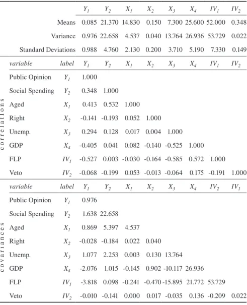
The data I use are publically available; public opinion in the International Social Survey Program ‘Role of Government’ and ‘Religion’ modules and social policy spending from the Organization for Economic Co-operation and Develop-ment ‘Social Expenditures Database’ covering 70 country-time points (across 1985-2006). I provide the variances and covariances necessary to estimate the main models. I include means only for didactic purposes (see Appendix 1-Table A1). All variable measurements and countries are in Appendix 1-Table A2, reproduc-ing Breznau (2017, p. 597). Almost all SEM software reads raw data or covariance matrix data (including correlation/variance matrices). Appendix 1-Table A3 pro-vides programming code (some call this “syntax”) for Mplus, Stata and R (RStudio running lavaan). Stata and R allow programming the matrix by hand, and Mplus reads a .dat file, which is a product of copying the matrix into a text editor and

sav-ing it with the file extension .dat10_.

I analyze models of opinion and policy reflecting Figure 3B with four inde-pendent X variables (aged population, right-party power, unemployment and GDP) predicting both Y outcomes. Table 1 presents results for M1, a model of free estima-tion with little theory and no addiestima-tional model constraints. Column “b” are unstan-dardized (‘metric’) coefficients, and “β” stanunstan-dardized coefficients. The results from Mplus here are identical to the other software except rounding error.

The results reveal how much Y₁ and Y₂ cause or explain each other’s

vari-ance. The standardized coefficient for Y2 predicting Y1 suggests that social policy

has a very large impact on public opinion (0.715), larger than public opinion has on social policy (0.084). However, according to standard testing the effects are insignificant. The insignificance of the smaller effect is perhaps not surprising but insignificance of the very large effect demonstrates the difficulty in disentangling reciprocal effects statistically. Moreover, the countries are not exactly a sample of a larger population, like with human populations. Cut-offs (e.g., p<0.05) are perhaps arbitrary without a sample population to generalize into. The t-statistic is still

use-ful for gauging the coefficients. Thus, Y2 impacting Y1 is more reliable and precise

(t=0.148/0.088=1.682) than vice-versa (at 0.357).

Scholars should exercise caution when interpreting effects independently. The relationship is a loop, not a single causal arrow. Here this loop accounts for (0.715*0.084=0.06) 6% of the joint distribution of the two Y variables (although this percentage also depends on the signs and scaling of the coefficients, see section “Explaining variance”). If correctly specified, social policy is a stronger compo-nent of this loop. In fact, the term field better describes this relationship because the forces are simultaneous and constant like magnets. The coefficients represent con-stant forces in this stable field. This contrasts with a cyclical loop where a change in

one variable sends effects looping through Y1 and Y2 in a cyclical process. A

steady-state force of the loop and a cyclical force running through the loop are different. To

say that the levels of Y1 on Y2 are at equilibrium because of their perpetual effects

Table 1 Results from M1. Freely Estimated Simultaneous Feedback between

Opinion and Policy

Y1 (public opinion) ON b s.e. β Fig 3B label

Y2 (social policy) 0.148 0.088 0.715 b

X₁ (aged) 0.024 0.116 0.052 c1

X2 (right) -0.659 0.656 -0.133 c2

X3 (unemp) -0.070 0.039 -0.264 c3

X₄ (GDP) -0.055 0.024 -0.287 c4

IV1 (FLP) -0.073 0.018 -0.540 e

Y2 (social policy) ON

Y₁ (public opinion) 0.403 1.129 0.084 a

X₁ (aged) 1.134 0.318 0.507 d1

X2 (right) -4.615 2.560 -0.194 d2

X₃ (unemp) 0.187 0.140 0.145 d3

X4 (GDP) 0.113 0.140 0.124 d4

IV2 (veto) -7.509 2.988 -0.235 f

variance std.variance

e.Y1 0.630 0.323 0.654 g

e.Y2 13.211 2.242 0.592 h

covariance correlation

(e.Y1,e.Y2) -1.878 1.213 -0.651 m

on each other is different than stating that causal effects between Y₁ on Y₂ unfold in specific, precise periods.

I do not rule out the cyclical version of feedback, but have specific theoretical arguments for a non-cyclical version, one that takes place without yearly-time con-sideration and is sufficiently complex to warrant SFMs. I might take interest in the cyclical relationship when investigating a specific social policy with specific time periods of voting or policymaking. But this macro-comparative exercise presumes that the sum of all specific instances contains common simultaneous feedback; i.e., not particular to one country-year. The comparative advantage here is the ability to test if the general process formulated in a theory of simultaneous feedback and positive returns can be explained by these data (Breznau, 2017; Pierson, 2000).

Without acknowledging reciprocal causality in some form, scholars might

measure a unidirectional effect of Y₁ on Y₂ and then separately estimate

unidirec-tional Y2 on Y1 rather than a SFM. Appendix 1-Table A4 reveals results from

sepa-rate regressions. The striking difference is that in both unidirectional regressions

the β-coefficients for Y1 and Y2 are close to 0.1. This approach leads researchers to

conclude that either public opinion explains or causes social policy (Y₁ causes Y₂)

or vice-versa (Y2 causes Y1), and in either case that the effect is around magnitude

of 0.1 standard deviations. Given a theory of simultaneous or reciprocal causality,

both conclusions are false and these models are misspecified11_{. The theory used}

in constructing M1, and the non-zero loop effect of 6% are evidence of this mis-specification.

Hypothesis Testing – The SEM Perspective

All parameters in M1 are free, showing how causal effects might look if I know

nothing theoretically about Y₁ and Y₂ feedback. Given a sufficiently detailed theory

of simultaneous feedback, a scholar knows something about the feedback. Thus, I test hypotheses derived from this knowledge. This is the structural equation mod-eler perspective focusing on overidentified models (Bollen, 1989). This perspective aims to test if a hypothetically derived model leads to something not far off from observational data. If the implied covariances of an overidentified model are not significantly different from observed covariances, then the hypothetical model may reflect the real-world data-generating processes. Testing hypotheses means compar-ing models with different exclusions or constraints to determine which fits the data better. Both model testing and model comparison require overidentified models.

Adding more instrumental variables achieves overidentification, as each adds one degree of model freedom. However, instrumental variables are rare and hav-ing two here represents the current limits of this research, beyond speculation (Breznau, 2013, p. 132; 136).

Fixing Parameters

Arguments for a reciprocal relationship of Y1 and Y2, are likely to include theory of

what this relationship looks like. This is true for opinion and policy feedback (Pier-son, 2000; Soroka & Wlezien, 2010). Thus, I specify hypotheses about the nature of the feedback and fix parameters to reflect this. The methodological advantage is an overidentified model. The theoretical advantages are testing competing hypotheses to construct improved theory.

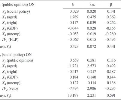
After reviewing the literature I determine that a thermostatic feedback theory

suggests that the standardized coefficient a (from Figure 3B) is negative 0.05 and b

is positive 0.30 (see Breznau, 2017). I fix the parameters to these values in M2. The SEM software analyzes only unstandardized effects, thus it is necessary to derive them by scaling the standard deviation of the standardized variable from one to

its observed value12_{. Meanwhile an increasing returns theory suggests that both}

coefficients are positive, possibly around 0.15 as specified in M3. The code is in Appendix 1-Table A5, and Table 2 presents the results.

The other variables’ coefficients do not carry much in the way of hypothesis testing (that comes in “Fit testing and diagnostics”); however, they should match

theoretical expectations. For example, if the coefficient for aged (X1) was large and

negative, I would become very suspicious that my model is misspecified because it is well-established that more older persons in a society requires far more social spending and usually means greater support of social spending.

A researcher might wish to fix an error term, covariance or mean instead of an

effect. M4 has a fixed Y2 error variance of 0.3, fixed covariance of Y1 and Y2 error

terms at zero and means of Y1 and Y2 at zero. I do not have theoretical arguments for

these constraints, they are didactic. Survey data provide the possibility to calculate measurement error for public opinion and I invent the number 0.3 here to represent this possibility. A fixed covariance of zero would be that the model represents a closed system accounting for all possible causal pathways between the variables. This would meet an experimental ideal, where the model explains all things that

cause Y1, Y2 and the causal loop between them. But this is highly unlikely in the

complex realm of cross-national survey research (see section “Instrumental

vari-12 Standardized effect formula: β * X Y

b σ

σ

= ; metric effect formula: * Y X

b β σ

σ

= ; where β = standardized coefficient, b = metric coefficient, σX = standard deviation of the

ables”). Nonetheless, I constrain it here for exercise. Means at zero is not important

theoretically, it just centers the expected values of Y1 and Y213.

Fit Testing and Diagnostics

Tests of fit determine how well a theoretically derived model explains real-world observations or compares with alternative models. There is a small universe of these tests. The art of ruling out alternative theoretical models is crucial to scien-tific utility (Hayduk et al., 2007; and discussed on the structural equation model-ing listserv SEMNET), and primarily comes from investigation of how close the

13 Researchers may have a theory that effects aandb are equal, but not have any predic-tion about their size. It is possible to constrain aandb to equality and let computer estimation decide what size is ideal in all three softwares (see A3-Appendix Three).

Table 2 Models of Competing Theories of Opinion-Policy Simultaneous

Feedback

M2 M3 M4

variable b s.e β   b s.e β   b s.e β

Y₁ (public opinion) ON

Y₂ (social policy) -0.010 - - -0.048 0.030 - - 0.146 0.030 - - 0.165 X1 (aged) 0.216 0.038 0.466 0.167 0.037 0.362 0.209 0.027 0.484

X₂ (right) -1.434 0.413 -0.291 -1.240 0.402 -0.252 -1.055 0.331 -0.229 X3 (unemp) -0.034 0.028 -0.129 -0.044 0.027 -0.165 -0.006 0.018 -0.023

X4 (GDP) -0.053 0.020 -0.281 -0.053 0.019 -0.282 -0.044 0.016 -0.249

IV₁ (FLP) -0.063 0.015 -0.471 -0.066 0.014 -0.494 -0.045 0.009 -0.358

Y₂ (social policy) ON

Y1 (public opinion) 1.500 - - 0.311 0.750 - - 0.154 0.750 - - 0.137

X₁ (aged) 0.901 0.211 0.403 1.062 0.207 0.474 1.175 0.164 0.495 X₂ (right) -3.376 2.264 -0.142 -4.217 2.225 -0.177 -3.929 2.211 -0.156 X3 (unemp) 0.172 0.142 0.134 0.183 0.140 0.142 0.245 0.121 0.180

X₄ (GDP) 0.210 0.104 0.229 0.148 0.103 0.160 0.201 0.080 0.206 IV2 (veto) -8.070 3.107 -0.252 -8.369 2.986 -0.261 -7.183 2.987 -0.212

e.Y1 0.446 0.075 0.466 0.424 0.072 0.445 0.300 - - 0.360

e.Y2 13.702 2.318 0.613 13.234 2.240 0.589 13.370 2.260 0.532

(e.Y1,e.Y2) -0.279 0.307 -0.113  -0.472 0.293 -0.199  0.000 - - 0.000

model-implied covariances come to the freely observed covariances in the data.

The proportion of explained variance (r2_{) is often a secondary concern. The term}

residual denotes the differences between model-implied covariances and observed

covariances. Residual also describes OLS error (in Yˆ), thus structural modelers

sometimes use fitted residuals or covariance residuals to adjudicate these concepts (Kline, 2011).

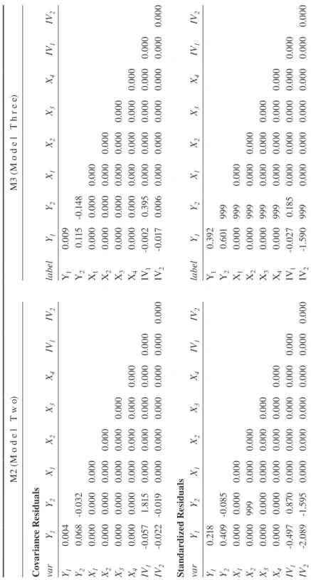
For just-identified models (like M1) the covariance residuals are zero as implied and observed are identical. In overidentified models, larger residuals sug-gest worse local fit. Scholars rely on standardized residuals and normalized resid-uals given that residresid-uals on their own do not have a common metric. Appendix 1-Table A6 provides residuals for M2 and M3. Smaller residuals support M3.

I might worry about the -1.28 normalized residual of IV2 and Y1 in M2

(Appen-dix 1-Table A6). This suggests unexplained covariance remaining between these variables, where none should be present. This might evidence a weak instrument. However, M3 is the preferred model where this residual is slightly lower at -0.964. Given that M3 fits well overall (as shown in Table 3), and that the theory sup-ports the instrument of veto points being exogenous to public opinion, I tentatively

defend IV2. Yet future research should search for other IVs. What causes policy

changes that does not cause opinion changes is a puzzle. Finding strong and valid instruments is a perpetual concern (Antonakis et al., 2010).

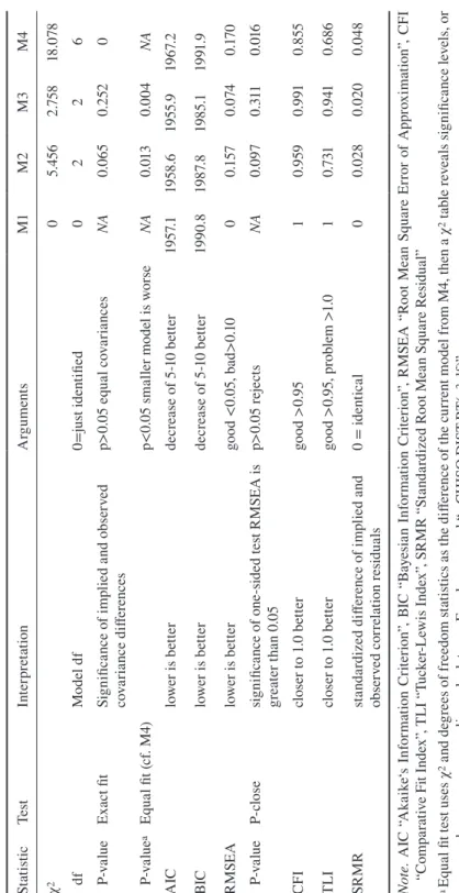
The model chi-square (_χ2_{) provides the primary statistic for evaluating}

global model fit. The _χ2 _{comes from maximum-likelihood estimation (for a good}

introduction see Kline, 2011, p. 199). The exact fit hypothesis is that implied and observed covariance matrices are identical except for random error. Put into test

terms, _χ2_{difference should not be significant at p<0.05, otherwise the matrices in}

comparison are significantly different offering evidence to reject this model. Thus, p>0.05 is a reasonable level to not reject the exact fit hypothesis. If this test passes,

it does not guarantee the strength of the IV, but asserts that nothing about the model

radically departs from the observed data; i.e., displays reasonable global fit. The exact fit test becomes increasingly likely to fail the larger the sample because it is more likely to pick up very small confounding parameters in the empirical realm. In macro-comparative survey research, having too large of a country sample is unlikely a problem. The equal fit hypothesis is that two implied covariance matri-ces do not differ from one another. If p<0.05 they are significantly different sup-porting the larger model (with less degrees of freedom). Note that models are only comparable with an equal fit test when they are nested; i.e., have all the same basic parameters and observational data.

There are several other global fit diagnostics. Considering all of them is

help-ful in selecting models, especially when they are not nested (Kline, 2011)14_{. Table}

Ta bl e 3 M od el F it S tat ist ics a nd T es ts St ati sti c Te st In te rp re ta tio n A rg um ent s M1 M2 M3 M4 χ 2 0 5.4 56 2.7 58 18 .0 78 df M od el d f 0= ju st i de nt ifi ed 0 2 2 6 P-v al ue Ex ac t fit Si gn ifi ca nc e o f i m pl ie d a nd o bs er ve d co va ria nc e d iff er enc es p> 0. 05 e qu al c ov ar ia nc es NA 0.0 65 0. 252 0 P-v al ue aEq ua l fi t ( cf . M 4) p< 0. 05 s m al le r m od el i s w or se NA 0.0 13 0.0 04 NA A IC lo we r i s b et te r de cr ea se o f 5 -1 0 b et te r 19 57. 1 19 58 .6 19 55. 9 19 67. 2 BI C lo we r i s b et te r de cr ea se o f 5 -1 0 b et te r 19 90 .8 19 87. 8 19 85 .1 19 91 .9 RM SE A lo we r i s b et te r go od < 0. 05 , ba d> 0.1 0 0 0.157 0.0 74 0.17 0 P-v al ue P-clo se sig ni fic anc e o f on e-sid ed t es t R M SE A i s gr ea te r t ha n 0 .05 p> 0.0 5 r ej ec ts NA 0.0 97 0. 311 0.0 16 CF I clo ser to 1. 0 b et ter go od > 0.9 5 1 0.9 59 0. 991 0.85 5 TLI clo ser to 1. 0 b et ter go od > 0. 95 , p ro bl em > 1.0 1 0.7 31 0. 941 0.6 86 SR M R   sta nd ar di ze d d iff er enc e o f i m pl ie d a nd ob se rv ed c or re la tion r es id ua ls

0 = i

de nt ic al 0 0.0 28 0.0 20 0.0 48 No te . A IC “ A ka ik e‘s I nf or m at ion C rit er ion ”, B IC “ Ba ye sia n I nf or m at ion C rit er ion ”, R M SE A “ Ro ot M ea n S qu ar e E rro r o f A pp ro xi m at ion ”, C FI “C om pa ra tiv e F it I nd ex ”, T LI “ Tu ck er -L ew is I nd ex ”, S RM R “ St an da rd iz ed R oo t M ea n S qu ar e R es id ua l”

a Eq

ua l fi t t es t u se s χ

2 an

d d eg re es of f re ed om sta tis tic s a s t he di ffe re nc e o f t he c ur re nt m od el f ro m M 4, th en a χ

2 ta

3 contains fit and diagnostics for models M1-M4, offering some preferable targets of these indices. I conclude that M3 is better than M1 because M1 does not have a strong theory to test and AIC and BIC are worse; and better than M2 because all fit indices (AIC, BIC, RMSEA, CFI and TLI) are better. Also, exact fit is less significant (0.252 vs. 0.065) and equal fit more significant (p-value 0.004) than M2 (0.013). It is better than M4, although M4 is just for example.

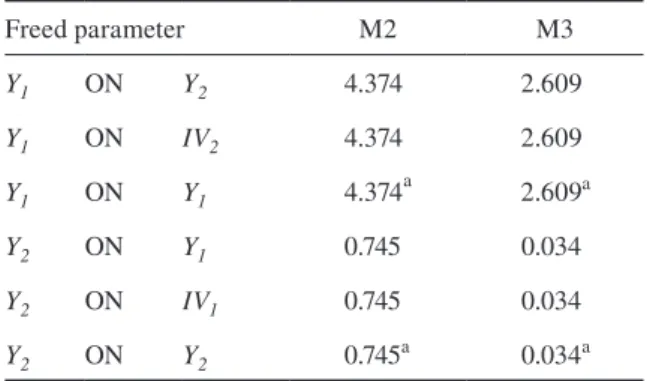
In addition to residuals, another tool to identify local misfit is modification indices. For every parameter in the model, the modification index is the change

in _χ2 _{if that parameter (coefficient or residual covariance) were freely estimated}

instead of estimated in its current form. The values are zero for parameters already freely estimated and take on positive values for parameters currently fixed (for

example the effect of IV1 on Y2 in all of the models). Appendix 1-Table A7 lists all

non-zero modification indices for M2 and M3. Appendix 1-Table A7 suggests that

estimating a free parameter for the regression of Y2 on IV1 is a way to improve the

model. The normalized residual between Y₂ and IV₁ is -1.28 (see Appendix 1-Table

A6) supporting this claim; however, a much larger gain in model fit would result

from adding a freely estimated coefficient for Y₁ on IV₂ (4.374 in M2) than for Y₂ on

IV₁ (0.745 in M2). This distinction is not evident from looking only at the residuals.

Yet, neither of these is possible because the model is not identified with the addition of either parameter (as per the rank condition discussed earlier). Here again are the current limits of this research.

Modification indices are agnostic statistical scores; they do not identify a theo-retical problem. Thus, simply freeing parameters in the model might defy, disrupt or debunk the causal model that the researcher carefully constructed using theory. Modification indices are a tool for researchers to use to re-visit their theories and discover what might be missing logically, before making any changes to the model. Focusing on M2: In Table A7, the modification indices are identical for the effect

of IV2 on Y1 and Y2 on Y1, and identical for IV1 on Y2 and Y1 on Y2. This

demon-strates how endogeneity works in the SFM. There is residual covariance between

Y₁ and Y2 (normalized value of 0.197 in M2) and the fit of the model may suffer as

a result, as the modification index of 4.374 suggests. This essentially means there is

a statistical relationship (covariance) between Y1 and Y2 not explained by the model

and if something could account for this unique feedback error, the model would fit

better; in this case a better or additional instrument for IV2. I did not discuss this in

Breznau (2017), but this is a useful finding from this excursus pointing at further research.

Explaining Variance

(effects a and b in Figure 3B and Table 1) running between Y₁ and Y₂. In M1, the

loop causal effect of Y2 on Y1 is not 0.715, but includes the effect of Y1 on Y2 of

0.084 as an indirect effect, and thus (0.715*0.084)=0.06. To calculate this effect

as a percentage, take 1/(1 – Y1* Y2) = 1/(1 – 0.06) = 1.064 = the original amount

plus 6.4% (Paxton, Hipp, & Marquat-Pyatt, 2011). One cycle through the feedback

loop produces about 6.4% of the endogenous variables’ covariance15_{. To this loop}

causal effect we may apply a Sobel-like test revealing a significance score (z-value)

of 0.13116_{. Interpretation is identical to a t-test making this statistic non-significant,}

which is not surprising given that the coefficients are not significant. Normally, another cycle would recover an additional 6% of 6% of the original covariance and so forth. In SFMs, there is no perpetual looping effect. One loop is the theoreti-cally specified ‘number of cycles’ for the SFM (Hayduk, 2009). The ideal model M3 has a loop causal effect of 2.25% (=0.03*0.75), lower than the 6% found in M1, but offering the best theoretical loop causal effect from this research based on fit diagnostics.

The loop causal effect only offers the amount of unique covariance explained by the loop. The remainder may be of interest to the researcher; however, the

amount of explained variance of Y1 and Y2, like their path coefficients, are

recip-rocally related17_{. The error of either Y variable actually contains part error and}

part non-error coming directly from the other endogenous variable’s error and thus violating the definition of error in OLS regression. The non-error part is not a com-ponent of the theory underlying the model, but an implication of the feedback loop.

Hayduk (2006) proposes a re-specification of r2 _{to resolve this problem called}

the blocked-error-r-square (beR2_{). Perfectly appropriate for SFMs, it equals the}

per-centage of variance explained by the model when excluding the other error term

as predictor (i.e., the non-error). The beR2 _{in M2 is (0.517/0.959=) 0.539 or 53.9%}

for Y₁ and (9.887/22.366=) 44.2% for Y₂, and for M3 the values are 56.1% for Y₁

and 41.7% for Y2 (see A3-Appendix Three). The results say little about differences

between the models; in fact, they point out that modeling two very different

theoret-15 The formula accounts for situations with opposite signed coefficients, or coefficients greater than one. As in any statistical model, all indirect effects should be calculated from unstandardized coefficients, thus the loop causal effect is (0.148*0.403)=0.06. Although the causal effect should be identical regardless of calculation method, always rely on unstandardized (‘metric’) coefficients.

16 The standard error (SE) of loop causal effect (where the two causal paths a and

b from Figure 3B are subscripted and normal font “b” is a metric coefficient) is: 2 2 2 2

ab a a b b

SE = b SE +b SE ; the significance test is then b b SEa b/ ab.

ical perspectives leads to similar explained variances. Given the small sample-size-to-variables-ratio, it is not surprising that these models explain so much variance.

I did not discuss this in Breznau (2017), that simultaneous feedback accounts for just over 2% of the joint distribution of public opinion and social spending. This would be trivial in standard r-square logic, but this is literally the explained variance unique to the loop itself. The feedback loop is like its own independent

variable explaining variance in Y₁ and Y₂. Moreover, this begs the question: what is

the loop? It represents the simultaneous impact of public opinion and social policy on one another. This simultaneity occurs in roughly one-year observation windows. Adding more observations should not change this if the loop is stationary at equi-librium. Therefore, disturbances to opinion or policy at best impart a 2% shift in the distribution of opinion and policy. If speaking in terms of majority elections this could make the difference in outcomes. In terms of social spending, this would impart an increase of 60 units (Dollars, Euro, Yen, etc) if a social benefit provides 3,000 units for something (pension, unemployment, etc). These potential outcomes suggest 2% may be non-trivial.

Further Considerations

Estimators

The task of the estimator is to identify what results most closely fit the implied covariance matrix to the observed covariance matrix (Myung, 2003). The most common estimator for this task is maximum likelihood (ML), or one of its many variants. In econometrics instrumental variables estimation often involves two- or three-stage least squares (2SLS or 3SLS) estimators. For SFMs, ML is the least biased estimator because it takes into consideration all information in the system (i.e., both equations) simultaneously. However, misspecification can lead ML to larger bias than 2SLS under some conditions (Paxton et al., 2011). This potential tradeoff suggests that the researcher may gain from running sensitivity checks with 2 or 3SLS to identify misspecification (Kirby & Bollen, 2009), but should not use the results because they are counter to a theory of simultaneity. 2SLS violates the

assumption that the errors are correlated (m in Figure 3) because it removes the

error through instrumental variable stages. However, as noted long ago by econo-mists, any adjustment to one outcome variable or its error term feeds back into the other and estimating the equations separately misses this process (Hausman, 1983, p. 194; Pearl, 2015).

The key is whether unobserved causes (and effects) are randomly distributed

with respect to the reciprocally causal relationship of Y1 and Y2. If they are not,

and should reconsider the formal model rather than worrying about estimators. The default in all three software packages and the default for researchers should be ML.

Disequilibrium

If there are meaningful changes in the size or direction of a causal force during the observation period, then SFMs may not be the appropriate tool. Kaplan, Harik and Hotchkiss (2001) demonstrate some risks associated with estimation under disequilibrium. They simulated different systems that experienced a shock before moving back to equilibrium. They took cross-sections out of the data series to esti-mate SFMs to test the severity of violating the equilibrium assumption. Their find-ings reveal that both regression coefficients representing the causal effects between

endogenous variables (c.f., Y1 and Y2 herein) change somewhat dramatically as the

system goes from the shock toward its equilibrium point. The error terms follow a similar pattern. The change in size of coefficients is gradual and smooth in the case of systems that move toward equilibrium without major fluctuations; however, when simulating a system with big oscillations the changes to the regression coef-ficients are sporadic if not chaotic. In either case, the problem is non-ignorable.

A researcher could mistakenly estimate model Figure 2A when in fact the

correct model is 2D wherein Y1,t-i shapes Y1,t-1 which leads to a new cycle of effects

between Y1 and Y2, and then Y1,t-1 takes on an entirely new causal effect on Y1,t

because of whatever transpired in the first loop (arrows between Y1 and Y2) at t-1.

This means that the model is cyclically recursive instead of nonrecursive (Billings & Wroten, 1978). Unfortunately, it is not possible to test for equilibrium, because the data needed for such a test are missing by definition. This leaves a strong bur-den on the researcher to argue for equilibrium. In the case of macro-comparative survey research, useful arguments may arise based on stable political and cultural systems. For example, the welfare states of Western Europe show a strong degree of stability in their political systems after the 1950s; whereas the Communist states of Eastern Europe broke down and experienced the shock of market transition in the 1990s.

the pooled data – as seen from a few basic fit indices. Nonetheless, the _χ2

p-value from the exact fit tests passes and it appears reasonable that effects are stable over time, for all non-missing years. The very small sample sizes are likely to blame for the troubling other indicators. I compare implied covariance matrices for M3 in

Appendix 1-Table A10. Here the main test variables in the model (involving IV1,

IV₂, Y1 and Y2) carry similar implied covariances across the two groups. A potential

problem is X4 (unemployment), which switches signs for some of the covariances

between the groups. This is evidence that further consideration should be given to this variable in future research to see if it is disrupting the stability of the system. Also, maybe there was a slightly different size of effects in Group 1 given the model fits the Group 2 data better; although, much more work is necessary here. This sensitivity analysis does not guarantee stability, and although this procedure is not an established method, it follows the art of structural equation modeling to pay detailed attention to model diagnostics.

Other Concerns

Missing values. Strictly speaking missing values should be dealt with in the estima-tion of the model as opposed to imputing them separately as if they were observed values. The reason for this is that missing values are subject to special measurement error and ignoring this can produce misleading results. However, contextual-level data are not observations in the strict sense of the word. Values for gross domestic product or level of democracy for example stem from complex calculations whose inputs are not necessarily identical across societies. Researchers at organizations such as the OECD take painstaking efforts to make these values as identical as pos-sible. These values do not represent objective qualities of societies in the way that observed variables such as age or height represent objective features of individuals. Contextual variables are instead more abstract. If they are missing it is best to take the nearest available year. The SFM is not suited for imputing values because of endogeneity.

and predicted latent scores that account for differential item functioning when there are three or more scale variables. In this example, previous research suggests

mea-surement invariance of the two ISSP questions (Andreß & Heien, 2001)18_{. Given}

that there are only two items, the loadings are equal. Thus, a predicted ‘factor’ is identical in variance with simply taking their mean as I did here.

Estimation without instruments. Several authors suggest estimating IV models without observed instrumental variables. Theoretically speaking this violates the exclusion restriction. These methods include estimating a latent or model-implied instrumental variable, or finding a subgroup of the total sample where a researcher can identify a causal instrument (Bollen, Kolenikov, & Bauldry, 2014; Ebbes et al., 2005; Heckman, Urzua, & Vytlacil, 2006; Heckman & Vytlacil, 1999). Suffice to say it is possible but not recommended.

Nonlinear models. If the endogenous variables are non-linear, SFMs are still possible using alternative regression estimation techniques. Simply resorting to lin-ear probability models may introduce new forms of bias (Finch & French, 2015; Terza, Bradford, & Dismuke, 2008)

Conclusion

This excursus shows that data limitations of macro-comparative research are not always a burden. With a theory of sub-yearly causal timing, scholars need not automatically reject cross-sectional survey data as a source for investigating their hypotheses. There are many theoretical forms of reciprocal causality for this. The simultaneous feedback model is only one form. Awareness of this method is not a sufficient condition to use it. Every step in the process of modeling simultaneous feedback must have theoretical argumentation behind it. Theory is a necessary con-dition for employing a simultaneous feedback model. Without a theory to specify the model, there is no identification of the reciprocal effects and probably no identi-fication of the model. Instrumental variables do not appear through random chance or out of thin air. Perhaps those normally running a bunch of correlations or regres-sions and then trying to explain the results may learn something from simultaneous feedback modeling, because theory is not ‘optional’ (Kalter & Kroneberg, 2014).

The impetus for bringing light to this method is the fact that so many macro-comparative phenomena in survey research appear to have reciprocal causality, and the forms of causality are highly complex and unfold in imprecise moments in time. There are well established methods, for example cross-lagged, fixed-effects/ random-slope, error correction and vector autoregressive models for fitting

dinal models. Given the correct research design it is possible to integrate simultane-ous feedback in a longitudinal model (Geweke, 1982) like an extension of Figure 2D. Whether or not simultaneous feedback can capture both lagged and instanta-neous processes is a theoretical consideration, one limited by available data. The loop causal effect from a SFM may then impact other outcomes (Hayduk, 1987). The loop itself acts as an independent ‘variable’ or a causal force, a consideration that researchers hopefully take away from this excursus.

There are limitations. Although data derive from individual-level sources, I am not aware of the possibility to model a SFM using multi-level techniques nor individual-level measurement models. Ideally, a measurement model is integrated into a path model for a fully parsimonious structural equation model. This would have a single variable for each survey item and their relationship with the latent scale (here public opinion), and it would have two levels of data analysis. Lacking degrees of freedom prevents the former, and a peculiarity of the SFM prevents the latter. The loop only exists at the aggregate level because there is no individual-level variance in social policy. Moreover, public opinion is by definition a group-level phenomenon, meaning strictly macro-group-level.

Theories germane to simultaneous feedback come in two broad types and both are debatable, so that researchers should use caution. The first type is where forces act upon each other simultaneously in the real world. The possibility of this is a philosophical argument. Some argue that by definition there are actions and reactions in the world, or that all things are reactions to other things. Meanwhile others argue that it is the interaction of objects and actions at the same point in time that constitute causal effects (Mulaik, 2009). Although this paper takes no philosophical position, researchers working with SFMs are by definition stepping on philosophical ground and tapping into debates that stretch throughout the his-tory of social thought. Thus, awareness of these arguments should help researchers defend themselves against epistemological attacks. The second type suggests that simultaneous causality exists without theoretically simultaneous forces, but can be inferred because the window of observation – usually something around a year in surveys – contains enough bi-directional causal forces between two phenom-ena that it is logical to treat them as simultaneously causal. This means that even though all these effects may run in different directions and have different sizes, that there is a sum or total effect in their causal loop force that is of theoretical and empirical interest.

exciting avenue for future implementation of simultaneous feedback in macro-com-parative survey data in general and specifically in the opinion-policy case.

References

Andreß, H.-J., & Heien, T. (2001). Four Worlds of Welfare State Attitudes? A Compari-son of Germany, Norway and the United States. European Sociological Review, 17(4), 337–356. http://doi.org/10.1093/esr/17.4.337

Angrist, J. D., Imbens, G. W., & Rubin, D. B. (1996). Identification of Causal Effects Using Instrumental Variables. Journal of the American Statistical Association, 91(434), 444– 455. http://doi.org/10.2307/2291629

Angrist, J. D., & Krueger, A. B. (2001). Instrumental Variables and the Search for Iden-tification: From Supply and Demand to Natural Experiments. Journal of Economic Perspectives, 15(4), 69–85. http://doi.org/10.3386/w8456

Antonakis, J., Bendahan, S., Jacquart, P., & Lalive, R. (2010). On Making Causal Claims: A Review and Recommendations. The Leadership Quarterly, 21(6), 1086–1120. http:// doi.org/10.1016/j.leaqua.2010.10.010

Bartels, L. M. (1991). Instrumental and “Quasi-Instrumental” Variables. American Journal of Political Science, 35(3), 777–800. http://doi.org/10.2307/2111566

Bascle, G. (2008). Controlling for endogeneity with instrumental variables in strategic ma-nagement research. Strategic Organization, 6(3), 285–327.

http://doi.org/10.1177/1476127008094339

Billings, R. S., & Wroten, S. P. (1978). Use of path analysis in industrial/organizational psy-chology: Criticisms and suggestions. Journal of Applied Psychology, 63(6), 677–688. http://doi.org/10.1037/0021-9010.63.6.677

Bollen, K. A. (1989). Structural Equations with Latent Variables. New York, NY: John Wiley & Sons.

Bollen, K. A. (2012). Instrumental Variables in Sociology and the Social Sciences. Annual Review of Sociology, 38(1), 37–72. http://doi.org/10.1146/annurev-soc-081309-150141 Bollen, K. A., Kolenikov, S., & Bauldry, S. (2014). Model-Implied Instrumental

Variab-le—Generalized Method of Moments (MIIV-GMM) Estimators for Latent Variable Models. Psychometrika, 79(1), 20–50. http://doi.org/10.1007/s11336-013-9335-3 Brehm, J., & Rahn, W. (1997). Individual-Level Evidence for the Causes and Consequences

of Social Capital. American Journal of Political Science, 41(3), 999–1023. http://doi.org/10.2307/2111684

Breznau, N. (2013). Public Opinion and Social Policy. Bremen, Germany: University of Bremen Library. https://elib.suub.uni-bremen.de/peid=D00103291

Breznau, N. (2016). Secondary Observer Effects: Idiosyncratic Errors in Small-N Secon-dary Data Analysis. International Journal of Social Research Methodology, 19(3), 301–318. http://doi.org/10.1080/13645579.2014.1001221

Breznau, Nate. 2017. Positive Returns and Equilibrium: Simultaneous Feedback Between Public Opinion and Social Policy. Policy Studies Journal 45(4), 583–612.

http://doi.org/10.111/psj.12171