ISSN: 1311-1728 (printed version); ISSN: 1314-8060 (on-line version) doi:http://dx.doi.org/10.12732/ijam.v31i6.3
THE ROLE OF TRANSFER FUNCTION IN THE STUDY OF STABILITY ANALYSIS
OF FEEDBACK CONTROL SYSTEM WITH DELAY D. Piriadarshani1§, S. Sathiya Sujitha2
1,2 Department of Mathematics
Hindustan Institute of Technology and Science Chennai 603 103, INDIA
Abstract: Loop delays appear obviously in several control applications. Due to loop delays, more complications arrive in feedback control systems. Loop delays cannot be avoided in a system controlled via communication networks as it decreases the stability of the system and restricts the achievable response time of the system. The transfer function is a main tool for analyzing and designing the feedback control system. It describes the system’s input output behaviour. In this paper, we have examined the stability of feedback control system using transfer function.
AMS Subject Classification: 34Dxx, 34D20, 34Hxx, 34H15
Key Words: stability, transfer function, feedback control system, long divi-sion method, Routh-Hurwitz method, impulse response
1. Introduction
Feedback control systems are usually mentioned as closed loop control systems. Delay is dangerous in feedback control system. The problem of time delay in the feedback loop has come into view in recent years. These delays may create the system’s performance bad or even cause the system unstable. Contribution of this paper is analyzing the stability of feedback control system using transfer
Received: May 18, 2018 c 2018 Academic Publications
function. It is used to describe the input-output relations of systems which can be characterized by linear, time-invariant, differential equations. It is an important tool for analyzing and designing the closed loop control system. The characteristic equation of closed loop system with delay will be of the form
A(s) +B(s)e−τ s= 0, whereτ is a delay. Then the transfer function for closed
loop system can be defined as G(s) = BA((ss)).
The following are the properties of transfer function:
• The transfer function is expressed only for a linear time-invariant system and it is not expressed for nonlinear systems.
• Initial conditions of the LTI system should be zero.
• The transfer function is not dependent of the input of the system.
A.A. Khan et al., gave the favorable effect of time delays on the tracking performance of a control system [1]. In 2013, F.A. Salem introduced control solution of basic open loop electric DC machines, two loop current and speed control of electric machines [2]. P. Hovel described the basic concepts and suggested a summary of the time delayed feedback scheme [3]. Piriadarshani et al., discussed about the stability of neutral delay differential equation with infinite delay in 2012, [4]. Sujitha et al. analysed the stability of a second order DDE which is expressed as a special case of the one-mass system controlled over network using Lambert W function [6].
2. Preliminaries
2.1. Poles and Zeros of Transfer Function
2.2. Impulse Response
An impulse response of a system g(t) is the inverse Laplace Transform of the transfer function G(s) of a system given by
g(t) =L−1(G(s)).
An another way of analyzing the stability of feedback control system is impulse response. A feedback control system has the following stability properties:
• A feedback control system is said to be asymptotic stable if limt→∞g(t)→
0.
• A feedback control system is marginally stable if 0<limt→∞g(t) <∞.
• A feedback control system is said to be unstable if limt→∞g(t)→ ∞.
2.3. Long Division Method
The following steps for analyzing the stability of feedback system with Long Division method will be constructed as follows:
• Constructing the transfer functionG(s) = BA((ss)). • Choosing the denominatorA(s).
• Creating two new polynomials A1(s) and A2(s).
• Form A1(s)
A2(s).
To system to be stable, all a1, a2, ... should be positive, otherwise it is unstable.
2.4. Routh-Hurwitz Method
3. Examples
In this section, we are providing examples of stability analysis of delayed res-onator and second order one-mass system controlled over the network.
3.1. Delayed Resonator
The delayed resonator (DR) is an absorber tuning approach which uses partial state feedback with time delay whose governing equation of motion is
mx¨(t) +cx˙(t) +kx(t) +gx(t−τ) = 0, (1)
where m - mass, c - damping parameter, k -stiffness parameter and x(t) -displacement,g - feedback gain, τ - delay.
In Delayed Resonator the delay is introduced due to the feedback control law. The characteristic equation of this feedback control system is
ms2+cs+k+ge−sτ = 0. (2)
It can be expressed in the general form of A(s) +B(s)e−sτ = 0. The transfer
function can be represented asG(s) = BA((ss)). Here
G(s) = g
ms2+cs+k,
where feedback gain g = p
(cw)2+ (mw2−k)2 and w > qk
m. The poles are
given by
s1= (−c)+
√
c2−4∗m∗k
2∗m and s2=
(−c)−√c2−4∗m∗k
2∗m .
Case i.
Supposem= 50kg;c = 2∗103kg/s;k = 2∗107N/m. Take w= 650 and hence
g= 1,719,193.12. The transfer function for the system described in (1) is
G(s) = 1,719,193.12
50∗s2+ (2∗103)∗s+ (2∗107).
The poles ares1 =−0.2000 + 6.3214i and s2 =−0.2000−6.3214i. As s1 and
s2 have negative real part, the above single-degree -of-freedom(SDOF) system is stable.
Case ii.
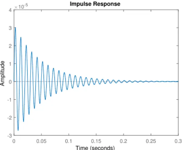
0 0.05 0.1 0.15 0.2 0.25 0.3 -3
-2 -1 0 1 2 3 4 10
-5 Impulse Response
Time (seconds)
Amplitude
Fig. 1. Impulse response for delayed resonator
From the above figure as limt→∞g(t)→0, the system represented by (1) is
asymptotically stable.
Case iii.
Here A(s) =ms2+cs+k. By the long division method, formulate two poly-nomials:
A1(s) =ms2+k and A2(s) =cs,
A1(s)
A2(s) = m
cs+
1
c ks
,
where a1 = mc and a2 = ck. For m = 50kg;c = 2∗103kg/s;k = 2∗107N/m,
a1 = 0.025 and a2 = 0.0001 are positive, then the roots ofA(s) lie in the left half plane.
The system represented by (1) is stable.
Case iv.
Considerm= 50kg;c= 2∗103kg/s;k= 2∗107. The characteristic polynomial is 50s2+ (2∗103)s+ (2∗107). Using the Routh-Hurwitz method, a Routh array is constructed as
s2 50 2∗107
s1 2∗103 0
s0 4∗1010
Values of an and bn Poles s1and s2 Nature of the System
an= 3>0, bn= 2>0 -2, -1 Stable
an= 1>0, bn=−2<0 1, -2 Unstable
an=−3<0, bn= 2>0 2, 1 Unstable
an=−1<0, bn=−2<0 2, -1 Unstable
Table 1: Stability Analysis based on the nature of Poles
3.2. Second Order System Controlled over the Network
Consider the second order system controlled over the network whose governing equation is
¨
y(t) +any˙(t) +bny(t) =u(t), (3)
wherean and bn are real numbers.
By control law with controller gainK is given by
u(t) =Ky(t−τ). (4)
Equation (3) becomes
¨
y(t) +any˙(t) +bny(t)−Ky(t−τ) = 0, (5)
whose characteristic equation is
s2+ans+bn−Kpe−sτ = 0.
Case i.
The transfer function for (3.3) is
G(s) = −Kp
s2+a
ns+bn
. (6)
Here A(s) =s2+a
ns+bn and B(s) =−Kp, and the poles are
s1 =
−an+
p a2
n−4bn
2 and s1 =
−an−
p a2
n−4bn
2 .
Case ii.
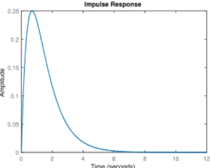
0 2 4 6 8 10 12 0
0.05 0.1 0.15 0.2 0.25
Impulse Response
Time (seconds)
Amplitude
Fig. 2. Impulse response of second order system controlled over the network for a= 3>0, b= 2>0
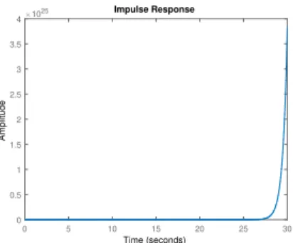
0 10 20 30 40 50 60
0 0.5 1 1.5 2 2.5 3 3.5
4 10
25 Impulse Response
Time (seconds)
Amplitude
Fig. 3. Impulse response of second order system controlled over the network for a= 1>0, b=−2<0
0 5 10 15 20 25 30
0 2 4 6 8 10
12 10
25 Impulse Response
Time (seconds)
Amplitude
0 5 10 15 20 25 30 0
0.5 1 1.5 2 2.5 3 3.5
4 10
25 Impulse Response
Time (seconds)
Amplitude
Fig. 5. Impulse response of second order system controlled over the network for a=−1<0, b=−2<0
From the above figures, we have the following table.
Values ofan and bn limt→∞g(t) Nature of the System
an= 3>0, bn= 2 >0 tends to zero Stable
an= 1>0, bn=−2<0 tends to infinity Unstable
an=−3<0, bn= 2>0 tends to infinity Unstable
an=−1<0, bn=−2<0 tends to infinity Unstable
Table 2: Stability Analysis using Impulse Response
Case iii.
From (6),A(s) =s2+ans+bn, by Long division method we formulate two
polynomials
A1(s) =s2+bn and A2(s) =ans,
Then, A1(s)
A2(s) = 1
an
s+ an1
bns
,
wherea1 = an1 and a2= anbn. Case iv.
By the Routh-Hurwitz method, let us construct the Routh array in the following table.
Values ofan andbn Values ofa1 and a2 Nature of the System
an= 3>0, bn= 2>0 a1= 0.3333, a2 = 1.5 Stable
an= 1>0, bn=−2<0 a1 = 1, a2 =−0.5 Unstable
an=−3<0, bn= 2 >0 a1 =−0.3333, a2 =−1.5 Unstable
an=−1<0, bn=−2<0 a1 =−1, a2= 0.5 Unstable
Table 3: Stability Analysis using Long Division Method
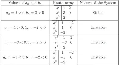
Values of an and bn Routh array Nature of the System
an= 3>0, bn= 2>0
s2 1 2
s1 3 0
s0 2
Stable
an= 1>0, bn=−2<0
s2 1 −2
s1 1 0
s0 −2
Unstable
an=−3<0, bn= 2>0
s2 1 2
s1 −3 0
s0 2
Unstable
an=−1<0, bn=−2<0
s2 1 −2
s1 −1 0
s0 −2
Unstable
Table 4: Stability Analysis using Routh-Hurwitz Method
4. Conclusion
The analytical stability of a feedback control system such as delayed resonator and second order system controlled over the network is analysed with the help of transfer function using various kinds of methods. Moreover the theory can be extended to higher order delay differential equation representing dynamical system.
References
[1] A.A. Khan, D.M. Tilbury and J.R. Moyne, Favorable effect of time delays on tracking performance of type-I control systems, IET Control Theory
[2] F.A. Salem, Dynamic modelling, Simulations and control of electric ma-chines for mechatronics applications,International J. of Control,
Automa-tion and Systems,1, No 2 (2013), 30-42.
[3] P. Hovel, Control of Complex Nonlinear Systems with Delay, Springer-Verlag, Berlin - Heidelberg (2010), DOI:10.1007/978-3-642-14110-2-2.
[4] D. Piriadarshani and T. Sengadir, Asymptotic stability of differential equa-tions with infinite delay,J. of Applied Mathematics 2012 (2012), Art. ID 804509, 10 pp.
[5] N. Olgac and M. Hosek, A new perspective and analysis for regenerative machine tool chatter,International J. of Machine Tools and Manufacture, 38(2013), 783-798.
[6] S.S. Sujitha and D. Piriadarshani, A Lambert W function approach for solution of second order delay differential equation as a special case of the one-mass system controlled over the network,International J. of