MJCCA9 – 660 ISSN 1857-5552 e-ISSN 1857-5625
Received: December 8, 2014 UDC: 548.73
Accepted: January 5, 2015 Review
X-RAY DIFFRACTION BROADENING ANALYSIS
Stanko Popović1,2*, Željko Skoko2
1
Croatian Academy of Sciences and Arts, Croatia
2
Physics Department, Faculty of Science, University of Zagreb, Croatia
[email protected]; [email protected]
The microstructural parameters of a crystalline sample can be determined by a proper analysis of XRD line profile broadening. The observed XRD line profile, h(ε), is the convolution of the instrumental profile, g(ε), and pure diffraction profile, f(ε), caused by small crystallite (coherent domain) sizes, by faultings in the sequence of the crystal lattice planes, and by the strains in the crystallites. Similarly, f(ε) is the convolution of the crystallite size/faulting profile, p(ε), and the strain profile, s(ε). The derivation of f(ε) can be performed from h(ε) and g(ε) by the Fourier transform method, which does not require mathe-matical assumptions. The analysis of f(ε) can be done by the Warren-Averbach method applied to the ob-tained Fourier coefficients. Simplified methods based on integral widths may also be used in studies where a good relative accuracy suffices. The relation among integral widths of f(ε), p(ε) and s(ε) can be obtained if one assumes bell-shaped functions for p(ε) and s(ε). Integral width methods overestimate both strain and crystallite size parameters in comparison to the Warren-Averbach method. The crystallite size parameter is more dependent on the accuracy in the diffraction profile measurement, than it is the strain parameter. The precautions necessary for minimization of errors are suggested through examples. The crystallite size and strain parameters obtained by means of integral widths are compared with those which follow from the Warren-Averbach method. Recent approaches in derivation of microstructure are also mentioned in short.
Keywords: X-ray diffraction broadening; crystallite size andstrain; deconvolution; integral width; Warren-Averbach method
АНАЛИЗА НА ШИРОЧИНАТА НА РЕНДГЕНСКИТЕ ДИФРАКЦИОНИ МАКСИМУМИ
Микроструктурните параметри на кристален примерок можат да се определат со помош на соодветна анализа на проширувањето на профилите од рендгенската дифракција. Регистрираниот дифракционен профил, h(ε), е конволуција на инструменталниот профил, g(ε), и чистиот дифракционен профил, f(ε), предизвикан од малите кристалитни димензии (кохерентен домеин), потоа од несовршеностите во секвенциите од рамнините на кристалната решетка и од напрегањата во кристалитите. Слично, f(ε) е конволуција на кристалитниот големина/несовршеност профил, p(ε), и профилот на напрегнатост, s(ε). Одредувањето на f(ε) може да се изврши од h(ε) и g(ε) со помош на методот на Фуриеова трансформација, којашто не бара математички претпоставки. Анализата на f(ε) може да се изведе со помош на методот на Warren-Averbach применета на добиените Фуриеови коефициенти. Упростените методи засновани на интегралните широчини на профилите можат, исто така, да се користат и при студии каде што се достигнати релативно добри согласности. Зависноста помеѓу интегралните широчини на f(ε), p(ε) и s(ε) може да се добие ако се претпостават ѕвоновидни функции за p(ε) и s(ε). Во споредба со методот на Warren-Averbach, методот на интегрална широчина ги преценува параметрите на напрегнатоста и на кристалитната големина. Параметарот на кристалитната големина е позависен од точноста на мерењето на дифракциониот профил во споредба со параметарот на напрегнатоста. Сугерирани се, низ примери, неопходните претпазливости за минимизирање на грешките. Параметрите на
кристалитната големина и на напрегнатоста добиени со помош на интегралната широчина се споредени со оние добиени со методот на Warren-Averbach. Накусо се наведени и неодамнешните сознанија во врска со определувањето на микроструктурата.
Клучни зборови: широчина на рендгенските дифракциони максимуми; кристалитна големина и напрегнатост; деконволуција; интегрална широчина; метода на Warren-Averbach
1. INTRODUCTION
Microstructural parameters of a given mate-rial, crystallite size, distribution of sizes, crystallite strain and stacking faults, can be determined by X-ray diffraction methods, in combination with other techniques, especially electron microscopy and dif-fraction. All information on microstructure is con-tained in its diffraction pattern and can be inferred by a proper decoding and interpretation of the pat-tern. As the crystallite size decreases below, say, 100 to 200 nm, and/or with the presence of strains, diffraction line profiles become measurably broad-er than the instrumental profile. The high angle dif-fraction lines are affected first, and the K12
spectral components eventually cease to be re-solved. For the crystallite size of, say, 10 nm, high angle diffraction lines become very broad and dif-fuse and may disappear, depending also on the fraction of strains. Low angle diffraction lines also become broad. The derivation of microstructure depends strongly on the accuracy of the X-ray diffraction line profile measurement and on the minimization of errors inherent in the measure-ment, e.g. [1].
The crystallite size derived from diffraction pattern is a measure of the average thickness (in direction normal to diffracting crystal planes) of domains within which diffraction is coherent. This size does not necessarily correspond to the size of individual particles in a powder or grains in a poly-crystal. Particles can be the single crystals, but each particle or grain may contain several dif-fracting domains. Therefore, it is very useful to combine X-ray diffraction with other techniques, such as transmission and scanning electron micros-copy.
If a metal or a ductile material is deformed by cold work or other (thermal) treatment, its dif-fraction lines broaden, indicating that a disorder is introduced into the material. The nature of these changes may be [2]:
– the initial crystal grains are broken up into small crystallites (coherently diffracting domains) of the size up to, say, 100 to 200 nm;
– the crystallites remain large, say 1 m in size or bigger, but they are deformed, or suffer some kind of faultings, or undergo both effects;
– the material consists of small (even na-nosized) crystallites, which are deformed and/or possess stacking faults, all these effects contrib-uting to the broadening of diffraction lines.
The cold work produces arrays of disloca-tions, which have the effect to subdivide the grains into much smaller crystallites, which are also re-ferred to as domains in literature. The domains may be mutually sufficiently disoriented that each domain diffracts incoherently with respect to oth-er/neighbouring domains. The dislocations also produce tensile and compressive strains within the crystallites.
The first step before any attempt to analyze diffraction line broadening is to correct the ob-served (broadened) X-ray diffraction line profile of the studied sample for instrumental effects. A care-ful scan of a suitable standard sample, showing a negligible physical broadening will define the in-strumental contribution to broadening. Details for standard specimen preparation are given in the literature, e.g. [3]. The most desirable approach in order to obtain the instrumental profiles is to an-neal the sample showing broadened diffraction lines. Namely, the centroids of the observed profile of the studied sample, h(ε), and of the instrumental
profile, g(ε), should be as close as possible. How-ever, the annealed studied sample does not always give satisfactorily narrow diffraction lines; in that case the application of a suitable certified standard reference material is recommended. Detailed pro-cedures for derivation of microstructural parame-ters are given in e.g. [4].
2. DECONVOLUTION
The observed X-ray diffraction line profile,
h(), is the convolution of the instrumental profile,
The variable ε measures the angular devia-tion of a point from the true Bragg angle 2Θ0; ε
and the auxiliary variable t have the dimension of
2Θ.
Similarly to (1), f() is the convolution of the
crystallite size/faulting profile, p(), and the strain
profile, s():
f
p t
s
t
dt. (2)The derivation of f() from (1) can be per-formed from the measured h() and g() by the Fourier transform method, usually cited as the Stokes method [6], where no assumption in the mathematical description of h() and g() is neces-sary [5]. A valuable feature of the Stokes method is that the broadening of the diffraction profiles due to the angular separation of the K12 spectral
components is automatically allowed for.
The analysis of line broadening is based on the appropriate analysis of f(ε) in terms of crystal-lite size/faulting and strain parameters. Profile functions can be defined in the complex form as to be applicable to asymmetrical profiles:
exp , exp , exp . M M M M M M t M t M t M th H t i
t
g G t i
t
f F t i
The profiles are defined in the angular inter-val from 2Θ-M to 2Θ+M [–M , M]. The interval
should be chosen wide enough that beyond it the intensity of h(ε) and g(ε) can be considered to have fallen to the background level.
The Fourier coefficients of two measured profiles, of the studied sample, h(ε), and of the standard sample, g(ε), are given by summations:
1 1 1 10 cos π ,
sin π ,
0 cos π ,
sin π .
M M M M re M im M re M im M t
H t h h h
t
H t h h
t
G t g g g
t
G t g g
It follows from the Fourier integral theorem that the real and imaginary Fourier coefficients of pure physical diffraction profile f(ε) are given by equations:
2
2
,
2
2
.re re im im im re re im
re im
re im re im
H t G t H t G t H t G t H t G t
F t F t
G t G t G t G t
2
2
,
2
2
.re re im im im re re im
re im
re im re im
H t G t H t G t H t G t H t G t
F t F t
G t G t G t G t
F(t) = [F2re (t) + F
2
im (t) ]
1/2 .
Hre (t), Him (t), Gre (t) and Gim(t) are the coefficients
of h() and g(), respectively. The profile f (ε) can be synthesized as
f () = Fre (0) + 2 Σ[Fre (t) cos(t/M) +
Fim (t) sin(t/M)], (3)
the summation being performed from t = 1 to t ', and t ' is that value of t for which
Fre (t > t ') and Fim (t > t ')
have fallen practically to zero.
It is important to choose the adequate back-ground level of the measured profile. There is a tendency to estimate the background level too high, due to overlapping of the adjacent diffraction lines and also due to the fact that for small crystal-lite size the tails of the diffraction line are rather long. The consequence is the so-called hook effect
in the dependence of F(t) on t: the obtained value of F(0) is smaller than it should be. This can be avoided by choosing the background level of the studied sample to be equal to that of the annealed, standard, sample.
If the physical broadening is small compared to the instrumental broadening, the deconvolution may become rather unstable. If h() is only, say, 20% broader than g(), that gives an upper limit of about 100 to 200 nm for the determination of the crystallite size.
Experimental errors in the measurement of
h() and g(), the finite angular interval in which the profiles are measured and the truncation of their tails may produce oscillations (ripples) of the derived ordinates of f(ε) at high values of ε in (3).
3. WARREN-AVERBACH METHOD
coefficients obtained by deconvolution [5,6,7]. Namely, each coefficient is the product of the crys-tallite size/faulting parameter and the strain pa-rameter, the latter depending on the order of dif-fraction maximum:
F(t) = Fcf (t)·Fs(t,hkl). (4)
That fact makes it possible to separate crys-tallite size/faulting parameter from the strain pa-rameter for small (several initial) values of t, by using two or more diffraction orders for the same set of crystal lattice planes (eg. hkl, 2h 2k 2l, 3h 3k
3l). The order t of the coefficients can be trans-formed into the orderL according to the relation
0
, 4 sin M sin
t
L
where L is the distance normal to the diffracting planes (hkl), having the interplanar spacing dhkl ,
being the wavelength of X-rays. For small values of L the following approximation is valid:
ln F(L,hkl) = ln Fcf (L) – 22L2e2LWA /(dhkl)2 (5)
The analysis, according to (4) and (5), pro-vides in principle information on the (surface-weighted) crystallite size, LWA, distribution of
sizes, deformation-twin faulting and the (averaged mean squared) strain over a distance L normal to diffracting crystal lattice planes. A series of plots of ln F(L,hkl) versus 1/(dhkl)
2
are constructed for different values of L. For a given value of L the intercept on the ordinate axis gives the size/faulting
coefficient, Fcf (L), while the slope gives the mean
squared strain, e2LWA. The (negative) initial slope
of the plot of Fcf (L) versus L, i.e., the first
deriva-tive of the plot at L = 0, is connected with the mi-crostructural parameters:
– dFcf (L)/dL = 1/LWA + 1/LfWA . (6)
LWA is the crystallite size, as defined by the
Warren-Averbach method, in the direction normal to the diffracting planes, whereas LfWA is the
con-tribution due to faultings on crystal lattice planes. In case that contribution due to faultings is small, the intercept of the initial slope of Fc(L) (subscript
f omitted) versus L with the abscisa axis equals
LWA. For a strain free sample, the analogous
in-tercept on the abscisa axis of the plot F(L,hkl) ver-sus L yields directly LWA in direction normal to
the diffracting planes. The crystallite size distribu-tion is given by the second derivative, d2Fc (L)/dL
2
.
The second derivative cannot be negative, as the crystallite size distribution is positive. It follows that the plot of Fc(L) versus L should be concave
upward, but never downward. If it happens that the plot is concave downward, i.e. the hook effect is present, this is an indication that the coefficient
F(0) is smaller than it should be. Since F(0) is proportional to the area of the profile f(), the reason for the hook effect may be the overestima-tion of the background level.
Contribution due to faultings in (6) may ap-pear for a material which can be regarded structur-ally to be composed of well-defined layers. The faultings are random crystallographic misplace-ments of successive layers, i.e. random deviations from the correct sequence of layers (crystal lattice planes) according to requirements of the space group. The faultings may occur as a result of cold work (deformation fault) or crystal growth (twin fault). Not all diffraction lines are broadened or similarly broadened by the presence of faultings. A detailed description of the derivation of the fault-ing probability and the nature of faultfault-ings are given in e.g. [5].
4. INTEGRAL WIDTH METHOD
On the other hand, simplified methods, which are based on the integral width, i, or
full-width at half maximum, 1/2 (FWHM), of f(), may
be used in studies where a relative accuracy suf-fices. Simple procedures for derivation of the width i from the measured widths Bi and bi of
h() and g(), resp., can be found in e.g. [2]. These procedures are based on the following equation which can be derived from (1):
Bi = bi i / ∫ g() f() d
Similarly, the integral widths i,pi and si
off(),p() and s(), resp., are connected by the equation
i = pi si / ∫ p() s() d
In order to obtain the relation among the widths of h(), g() and f(), or among the widths of f(), p() and s(), one may assume bell-shaped functions for g() and f() in (7), or for p() and
Rietveld refinement and in the crystal structure analysis, are:
– Cauchy (Lorentzian) function,
1 2 21 C
C K , in literature used for p() in case of a wide crystal-lite size distribution;
– modified Cauchy function,
2 2 21 Q
Q K , used for s();
– Gauss function, exp
2 2
GG K , used for s();
– 2 2
sin S S
S K K , used for p() in case of a narrow crystallite size distribution;
– Voigt function, V(), used for both p() and s() [8] ;
– pseudo Voigt function, Vp
C
1
G ,
01 [9].
The Voigt function, a convolution of the Cauchy and Gaussian functions, appears to be a better choice in description of both size and strain profiles [8, 10, 11]. The derived (volume-weighted) crystallite size parameter, Lhkl, and the
(upper limit of) strain parameter, ehkl, depend on
assumptions for p() and s(), e.g. [12, 8, 13].
For instance, if p() is described by the Cau-chy function and s() by the Gauss function, the following approximate relation, derived from (8), can be used [14, 15]:
i2ipisi2. (9)
By using the well-known Scherrer equation (in case the stacking faults broadening is negligi-ble),
pi
Lhklcos
, and the Wilson equation,si 4ehkltan (where ehkl = d/ d , d is the
average spacing and d its change due to the strain), it follows from (9):
22 2 2
sin Lhklsin 4ehkl
, (10)
where icos. All available diffraction
or-ders from a given set of crystal lattice planes (or all diffraction maxima in case of a cubic sample) can be used to construct the linear plot
2 sin2
against sin2. The size and strain parameters are found from the slope,
Lhkl, and the ordinate intercept,
4ehkl
2 [16, 13].The shape of the crystallites may be as-sumed in case the integral width varies with the indices of diffraction lines. Let the mean shape of hexagonal crystallites be plate-like, which
thick-ness (in the direction of c axis) is much smaller than the base diameter (in the direction of a axis). In such a case, diffraction lines 00l are much broader than the lines hk0, while the lines hkl are intermediate in broadening.
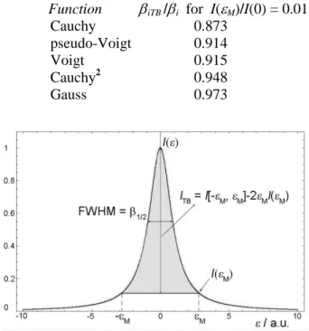
Both approaches, Warren-Averbach and in-tegral width methods, depend, among others, on the estimated background level along the diffrac-tion pattern and on the inevitable truncadiffrac-tion of diffraction profile tails. The truncation-background level error distorts the Fourier coefficients of the diffraction profile and may contribute to the hook effect introducing errors in the size and strain pa-rameter values ([5]). Instead of the theoretical val-ue, i = I [
_
, + ]/I(0), the measured value is iTB
= i –MM – 2M I(M )/I(0). iTB is the
truncat-ed integral width with the background below the profile subtracted (Fig. 1). In case –M andM are
the points where the profile ordinates fall to the one hundredth of I(0) (this choice was arbitrary and corresponds to an average detection limit in intensity measurement), the following combined truncation-background level errors are obtained for the bell-shaped functions [17, 18]:
Function iTB /i for I(M)/I(0) = 0.01
Cauchy 0.873
pseudo-Voigt 0.914
Voigt 0.915
Cauchy2 0.948
Gauss 0.973
Fig. 1. A bell-shaped function with parameters used in the text.
error is the biggest for C() (12.7 %), and the smallest for G() (2.7 %). The error for V() and
Vp() (8.5 %) is in between of those for C() and
G(), as expected. This is in agreement with ex-perimental evidence: the crystallite size is more affected by the accuracy with which the profile tails are measured than it is the strain.
5. EXAMPLES
Two cases of high symmetry, cubic, samples are presented: strain-free MgO showing only crys-tallite size broadening; NiO showing both crystal-lite size and strain broadening [17, 18]. In these cases, precautions for minimization of the com-bined truncation-background level error were un-dertaken. The influence of the background level error on the integral width, and consequently on the crystallite size and strain parameters, was found for a pure diffraction profile obtained by the Stokes method. Also, the broadening of diffraction lines which takes place during the phase transition
-In2Se3↔-In2Se3 is described briefly [19, 20].
The next example is the process of graphitization of the petroleum coke where all causes of broad-ening are present [21].
According to Warren [5], the background level of the broadened profile, h(), should be equal to the level of the instrumental profile, g(). This statement appears to be a very good approxi-mation and was applied in the following examples. Diffractometers with adequate X-ray optics and narrow slits provide rather sharp profiles g(), and their background level can be estimated with a satisfactory accuracy.
5.1. MgO
MgO (Fm3m, Z = 4, a = 0.4213(1) nm at 25 °C) was prepared from basic magnesium carbonate by calcination from 600 to 1300 ºC for 6 hours, followed by slow cooling inside the furnace to RT, in order to anneal strains. The widths of diffraction lines decreased as the calcination temperature in-creased. MgO1300 showed very sharp diffraction
lines, being practically as sharp as those of pure Ge (having micrometre sized grains) for which it was proved to represent the instrumental broadening. Therefore, line profiles of MgO1300 were used as
g()'s in deconvolution of the line profiles of MgO600 to MgO1000 by the Stokes method. Five
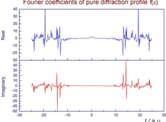
line profiles were analyzed, 200, 220, 222, 420 and 422. The Fourier coefficients obtained by decon-volution usually irregularly oscillate at higher
orders (Fig. 2). If all as-calculated Fourier coeffi-cients, shown in Figure 2, were used in the synthe-sis of f(), atotallyinadequate result would be ob-tained.
Fig. 2. As-calculated Fourier coefficients of pure diffraction profile, f(), for 200 MgO650
Therefore, all as-calculated Fourier coeffi-cients cannot be used either in the synthesis of a proper f() or in the Warren-Averbach method. Instead, only low order as-calculated (say, first 20 to 40) coefficients, which gradually decreased as their order increased, were used. When they started to oscillate (say, above the 20th to 40th order), they were extrapolated asymptotically to zero as their order increased (Fig. 3). By using the coefficients selected in such a way, proper f()'s were obtained, which could be nicely fitted by a Voigt function. The line profiles h(), g() and f() for the diffrac-tion line 200 are shown in Figure 4 (dots: meas-ured values for h() and g(), calculated values for
f(); full lines: fitting by a Voigt function) and for the diffraction line 422 in Figure 5.
Fig. 4. The line profiles 200 of MgO: h() – MgO650, g() – MgO1300 , and f() obtained by the Stokes method; dots: measured values for h() and g(), calculated values for f();
full lines: fitting by a Voigt function
Fig. 5. The line profiles 422 of MgO: h() – MgO600, g() – MgO1300 and f() obtained by the Stokes method
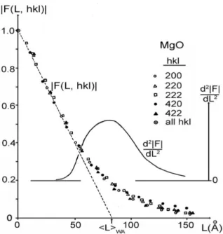
Fig. 6. Fourier coefficients F(L, hkl) vs L for five profiles of MgO600 obtained by the Stokes method; crystallite size
and crystallite size distribution derived by the Warren-Averbach method
The Fourier coefficients, F(L, hkl), for the five line profiles vs L are shown in Figure 6. One can notice that all F(L, hkl)'s lie practically on the same curve. Therefore, it can be concluded that the small crystallite size was the only cause of diffrac-tion broadening. Figure 6 also shows the value of the crystallite size, LWA, and the approximate
crystallite size distribution, d2F(L)/dL2, derived by the method of Warren and Averbach. The hook effect was practically absent, which means that the background level was not overestimated. The de-scribed procedure is a proof that the Stokes meth-od, if performed properly, yields f()'s with mini-mum approximations.
Having calculated the Fourier coefficients of
f()'s,i's wereobtained by equation
Fre(0)(2ΘM – 2Θ–M)/f(0), (11)
Fre(0) being the zero cosine Fourier coefficient.
The-se i's were used to calculate the crystallite size by
using the Scherrer equation, Lhkl
icos
. The values of Lhkl were 15% bigger (as expectedaccording to the literature, e.g. [13]), than LWA,
but similar for various hkl. The values of i's
ob-tained by (11) were used to construct the plot ac-cording to equation (10) for MgO600, shown in
Figure 7.
A straight line through the origin was ob-tained, this meaning that no strains were present in the sample. A crystallite size Lhkl of 10.0(5) nm
was obtained from the slope of the straight line. As the calcination temperature of MgO increased from 600 to 1000 ºC, the crystallite size increased from 10 to 44 nm, while the specific surface area de-creased from 50 to 16 m2/g.
Fig. 7. The application of equation (10) on five profiles of MgO600; Lhkl = 10.0(5) nm; bars indicate estimated
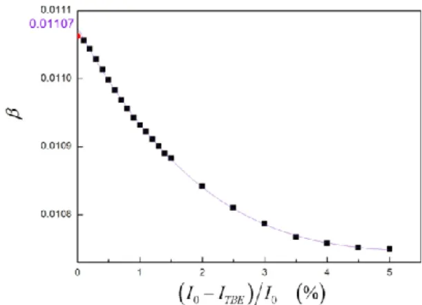
In order to find out the dependence of the in-tegral width on the background level error for pure diffraction profile, obtained by the Stokes decon-volution, the background level was intentionally overestimated up to 5 %, in steps of 0.1 to 0.5 %. Of course, both the integral intensity of the profile (that is, the surface under the profile) and the in-tensity maximum of the profile decreased with the progressive overestimation of the background lev-el. But, the decrease of the integral intensity was found bigger than the decrease of the maximum intensity. Therefore, the integral width decreased (for 3%) with the overestimation of the back-ground level (for 5%). The corresponding results for pure diffraction profile f() of MgO650, obtained
by the Stokes method (Fig. 4), are shown in Figure 8. That dependence was fitted by a third order pol-ynomial function. The extrapolation of that de-pendence to the point of zero background level overestimation may yield a true background level of diffraction profile; this procedure thus elimi-nates a possible initial error in the background level. The corresponding dependence of the crys-tallite size on the background overestimation is shown in Figure 9 [17, 18].
Fig. 8. Dependence of the integral width of pure diffraction profile f() of MgO650, obtained by the Stokes method (Fig. 4.), on the relative overestimation of the background level
Fig. 9. Dependence of the crystallite size of MgO650 (Figs. 4, 8) on the relative overestimation of the background level
5.2. NiO
NiO (Fm3m, Z = 4, a = 0.4177(1) nm at 25 °C) obtained from Ni(OH)2 by thermal
decompo-sition showed rather broad diffraction lines. Dif-fraction lines of Ge powder, intimately mixed with NiO, were used as g()'s. As i's of NiO, deduced
by the Stokes method (following the procedure described above for MgO), did not vary with either as 1/cosortan, it was concluded that both small crystallite size and strain caused broad-ening. The application of equation (10) on three diffraction line profiles is shown in Figure 10. It may be proposed that the hexagonal plates of Ni(OH)2 split into layers of NiO by the thermal
treatment at moderate temperatures; more details are given in [22].
Fig. 10. The application of equation (10) on three profiles of NiO; Lhkl = 8.3(5) nm, ehkl = 6.0(5) × 10–3; bars indicate
estimated standard deviations
5.3. Phase transition -In2Se3↔-In2Se3
In2Se3 exhibits at least four polytypic phase
transitions in the interval from low temperature to the melting point [19, 20]. The transition -In2Se3↔-In2Se3 as detected by X-ray diffraction is
shown in Figуре 11. Crystal data for these two phases are:
In2Se3: R3 m, Z = 3, a = 0.4025(5),
c = 2.8762(7) nm at 25 °C,
In2Se3: R3 m, Z = 3, a = 0.4000(8),
c = 2.833(1) nm at 205 °C.
the transition -In2Se3 -In2Se3 takes place
above 200 °C, while the reversal transition, -In2Se3 -In2Se3, below 80 °C. These
tempera-tures depend on the synthesis and previous history of the sample. For a polycrystalline sample, having highly oriented grains, the transition -In2Se3
-In2Se3 may take place between 80 and 50 °C, while
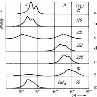
a powdered sample can be undercooled and be stable in the -phase below the room temperature. The broadening of diffraction lines is pronounced during the phase transitions indicating an increased disorder inside crystallites. The separation of the spectral doublet CuK12 is hardly visible during
the transitions. That separation is increased a little at temperatures before and after phase transitions.
Fig. 11. Diffraction line 0 0 27 of In2Se3 at different temperatures, exhibiting broadening during the phase
transition -In2Se3 ↔ -In2Se3
5.4. Graphitization of petroleum coke
This process represents a gradual transition from the petroleum coke toward the non-graphitic carbon, the graphitic carbon and the crystalline graphite (P63/mmc, Z = 4, a = 0.2460(1), c =
0.6708 (2) nm at 25 °C) during a gradual increase of temperature. Petroleum coke consists of minute grains in which there are several (say, ten) roughly parallel layers, having a diameter of 3 to 4 nm, which are mutually randomly oriented about the layer normal. X-ray diffraction pattern is typical for a random layer structure [5], showing symmet-rical broad lines 002 and 004 and asymmetsymmet-rical 2D bands 10 and 11 (Figs. 12a, 12b). As the tempera-ture increases, the 2D bands sharpen and move
toward smaller Bragg angles, but retain their asymmetrical shape. This indicates an increase of the layer diameter; however, the layers remain in random mutual orientation. The lines 002 and 004 also sharpen with temperature and shift toward higher Bragg angles, indicating a decrease of strains and an increase of number of layers in grains. Above 1600 °C a very broad line 006 also appears in diffraction pattern. After heating to 1500 °C and to 2150 °C the average interlayer spacing decreases to 0.3440 nm and to 0.3425 nm, resp., as measured at room temperature.
Fig. 12a. Parts of X-ray diffraction patterns of nongraphitic and graphitic carbons heated at high temperatures (patterns
taken at room temperature after cooling)
Fig. 12b. Parts of X-ray diffraction patterns of nongraphitic and graphitic carbons heated at high temperatures (patterns
taken at room temperature after cooling)
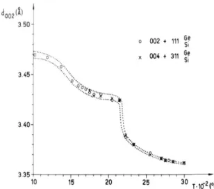
shows a beginning of splitting of 2D bands into 3D lines: 10 into 100, 101 and 102, and 11 into 110 and 112 (Figs. 12a, 12b). These modulations indi-cate the start of graphitizaton. The neighbouring layers, having reached the diameter of ~10 nm, begin to undergo mutual graphitic ordering. Also, diffraction lines 00l shift abruptly toward higher Bragg angles, indicating an abrupt decrease of the interlayer spacing (Fig. 13). As the temperature increases further, up to 3000 °C, all diffraction lines sharpen, due to an increase of the crystallite size and their further ordering (a decrease of strains), approaching the structure of highly crys-talline graphite (Fig. 14). The interlayer spacing gradually approaches the value typical for graphite. The fraction of layers involved in faultings falls from 1 to 0.15 upon heating from room tempera-ture to 3000 °C [21].
Fig. 13. The interlayer spacing, d002, of nongraphitic and graphitic carbons heated at high temperatures (measured at
room temperature after cooling)
Fig.14. The crystallite size (in direction normal to the graphite layers) determined by the methods of Warren and Averbach, LcWA, and Scherrer, Lc,and the lattice strain, (e
2
LWA) 1/2
, of nongraphitic and graphitic carbons heated at high temperatures
(all measured at room temperature after cooling)
6. OTHER APPROACHES
The described methods for interpretation of diffraction broadening have been developed before the introduction of sophisticated instrumentation and fast computers. Nowadays, reliable diffraction data can be collected by a modern diffractometer and the decovolution can be performed in a very short time. For instance, the Stokes deconvolution followed by the Warren-Averbach and integral widths analyses has been implemented in easy-to-use program, XBroad, for a quick determination of the basic microstructural information from X-ray powder diffraction patterns [23].
The introduction of analytical functions to fit diffraction line profiles has been a great ad-vancement in interpretation of diffraction patterns. That has led to the development of the Rietveld method [24], to diffraction pattern decomposition techniques [25] and to the general concept of the
whole powder pattern fitting (WPPF), e.g. [26]. The whole powder pattern modelling
(WPPM) allows a simultaneous processing of the whole X-ray diffraction pattern; it is based on a suitable model of domain size/shape and strain, without using arbitrary analytical profile functions,
e.g. [27]. These new approaches have been proved to be very useful.
The known crystal structure of a given sub-stance can be refined, e.g., as a function of temper-ature or pressure, using the Rietveld method. That method is a so-called full pattern analysis tech-nique. A model of the crystal structure, together with instrumental and microstructural information, are used to generate the theoretical diffraction pat-tern that can be compared to the observed patpat-tern. The least squares procedure is then used to mini-mize the difference between the calculated pattern and the observed pattern by adjusting model pa-rameters. That procedure may result in determina-tion of the crystal structure and microstructural parameters; however, it is rather challenging due to the overlap of diffraction lines in the X-ray powder diffraction pattern.
REFERENCES
[1] R. Delhez, Th. de Keijser, E. J. Mittemeijer, Accuracy of crystallite size and strain values from X-ray diffraction
line profiles using Fourier series; In: Accuracy in
Pow-der Diffraction, NBS Special Publication No. 567, S. Block, C. R. Hubbard (Eds), Washington DC, National Bureau of Standards, 1980, pp. 213–253.
[2] H. P. Klug, L. E. Alexander, X-ray Diffraction Proce-dures, New York, John Wiley, 1974.
spec-imen for X-ray diffraction line-profile analysis, Powder Diffraction 10, 129–139 (1995).
[4] D. Balzar, N. Audebrand, M. Daymond, A. Fitch, A. Hewat, J. I. Langford, A. Le Bail, D. Louër, O. Masson, C. N. McCowan, N. C. Popa, P. W. Stephens, B. Toby, Size-strain line-broadening analysis of the ceria round-robin sample, J. Appl.Cryst. 37, 911–924 (2004). [5] B. E. Warren, X-ray Diffraction, Reading, MS,
Addison-Wesley, 1969 / Dover, NY, Mineola, 1990.
[6] A. R. Stokes, A numerical Fourier-analysis method for the correction of widths and shapes of lines on X-ray powder photographs, Proc. Phys. Soc. London, 61, 382– 391 (1948).
[7] B. E. Warren, B. L. Averbach, The effect of cold-work distortion on X-ray patterns, J. Appl. Phys. 21, 595–599 (1950).
[8] J. I. Langford, A rapid method for analysing the breadths of diffraction and spectral lines using the Voigt function,
J. Appl. Cryst.11, 10–14 (1978).
[9] P. Thompson, D. E. Cox, J. B. Hastings, Rietveld refine-ment of Debye-Scherrer synchrotron X-ray data from Al2O3, J. Appl. Cryst.20, 79–83 (1987).
[10] J. I. Langford, Diffraction line broadening analysis; In:
Accuracy in Powder Diffraction, NBS Special Publica-tion No. 567, S. Block, C. R. Hubbard (Eds), Washing-ton DC, National Bureau of Standards, 1980, pp. 255– 269.
[11] J. I. Langford, Use of pattern decomposition or simula-tion to study microstructure: theoretical considerasimula-tions: In: IUCr Monographs on Crystallography, Defect and Microstructure Analysis by Diffraction, R. L. Snyder, J. Fiala, H. J. Bunge, (Eds), Oxford, Oxford University Press, 1999, pp. 59–81.
[12] W. Ruland, The separation of line broadening effects by means of line-width relations, J. Appl. Cryst.1, 90–101 (1968).
[13] D. Balzar, S. Popović, Reliability of the simplified integral-breadth methods in diffraction line-broadening analysis, J. Appl. Cryst.29, 16–23 (1996).
[14] F. R. L. Schoening, Strain and particle size values from X-ray line breadths, Acta Cryst.18, 975–976 (1965).
[15] N. C. Halder, C. N. J. Wagner, Separation of particle size and lattice strain in integral breadth measurements,
Acta Cryst. 20, 312–313 (1966).
[16] S. Popović, Application of bell-shaped functions in X-ray diffraction broadening analysis, Croat. Chem. Acta 57, 749–755 ( 1984).
[17] S. Popović, Ž. Skoko, G. Štefanić, Factors affecting diffraction broadening analysis, Z. Kristallogr. Proc. 1, 55–62 (2011).
[18] Ž. Skoko, S. Popović, G. Štefanić, Dependence of mi-crostucture on errors in X-ray diffraction profile meas-urement, J. Mater. Sci. Eng.A3,690–697 (2013). [19] S. Popović, B. Čelustka, D. Bidjin, X-ray diffraction
measurement of lattice parameters of In2Se3, Phys. Stat. Sol. A 6, 301– 304 (1971).
[20] S. Popović, A. Tonejc, B. Gržeta, B. Čelustka, R. Troj-ko, Revised and new crystal data for indium selenides, J. Appl.Cryst.12, 416–420 (1979).
[21] S. Popović, Analysis of X-ray diffraction line broaden-ing, Izvj. Jugoslav. centr. krist., Yugoslav (Croatian) Academy of Sciences and Arts12, 47–80 (1977). [22] C. L. Cronan, F. J. Micale, M. Topić, H. Leidheiser Jr.,
A. C. Zettlemoyer, S. Popović, Surface properties of Ni(OH)2and NiO, J. Colloid Interface Sci. 55, 546–557 (1976).
[23] Ž. Skoko, J. Popović, K. Dekanić, V. Kolbas, S. Popo-vić, XBroad–program for extracting basic microstructure information from XRD pattern in few clicks, J. Appl. Cryst.45, 594–597 (2012).
[24] R. A. Young, The Rietveld Method. Oxford, Oxford University Press, 1993.
[25] J. I. Langford, D. Louër, Powder diffraction, Rep. Prog. Phys. 59, 131–234(1996).
[26] P. Scardi, A new whole-powder pattern-fitting approach: In: IUCr Monographs on Crystallography, Defect and MicrostructureAnalysis by Diffraction, R. L. Snyder, J. Fiala, H. J. Bunge (Eds), Oxford, Oxford University Press, 1999, pp. 570–596.
[27] P. Scardy, M. Leoni, Y. H. Dong, Whole powder pattern modelling, IUCr Commission on Powder Diffraction,