Probabilistic Activity Recognition in Navigation

Probabilistic Activity Recognition in Navigation

Octavi Font

and Guillem Franc`es

and Anders Jonsson

Dept. Communication and Information Technologies Universitat Pompeu Fabra

Barcelona, Spain

Phil Bartie

University of Stirling Stirling, United Kingdom

William Mackaness

Abstract—In this paper we present a novel probabilistic approach to activity recognition. Our approach is to estimate posterior probabilities of different activities using Bayes’ rule. The approach can handle any type of activities as long as it is possible to estimate the conditional probabilities of potential observations, and easily scales to large numbers of activities. We test our approach empirically in an environment where observations are GPS signals of users moving around in a city.

I. INTRODUCTION

Activity recognition is the problem of inferring the intent of a given user or group of users through observation of their behavior. Activity recognition is a form of cognitive inference since the intent of a user is unobservable to anyone except the user itself. Sensors typically include GPS signals, cameras, accelerometers, gyroscopes or any other devices that can help disambiguate a user’s activity.

In this paper we present a Bayesian approach to activity recognition. In our approach, each activity has an associated likelihood of being the activity currently pursued by the user, i.e. a normalized posterior probability that is updated as a result of each new observation. An algorithm for activity recognition can either output the most likely activity or a list of the most likely activities together with their relative likelihood. Our approach has two main advantages: it is independent of the actual activities and sensors used in a particular instance of activity recognition, making it a flexible choice with potential use in many different applications. The only specification that the algorithm needs as input is the conditional probability of making a certain observation given a particular activity, which can either be provided by a system expert or estimated experimentally. Our approach also appears to scale very well to instances that include many thousands of different activities. We implement our approach as part of a system that relies solely on GPS signals to track a single user. Our system consists of two modules: a city model representing the geo-graphical area in which the user is moving, and a recognition module that receives as input a sequence of GPS signals and outputs a ranking of the user’s most likely activities.

Existing approaches to activity recognition using GPS sig-nals include hierarchical conditional random fields [1] and clustering to detect recurring patterns of visiting locations [2], [3]. Several researchers have also applied data mining to trajectory data, using the information to build ontologies [4],

[5], [6], [7], [8] or simply to extract meaningful patterns [9]. A similar idea to ours was proposed in the more restricted context of visual recognition from images [10].

The rest of the paper is organized as follows. In Section II we present the methodology behind our approach. In Section III we describe our framework for testing the approach exper-imentally. Section IV presents results of experiments, while Section V concludes with a discussion about future work.

II. METHODOLOGY

Accurately estimating the current activity of a user is a challenging problem since many variables are unobservable. Depending on the sensors used, it may be hard to establish precisely what the user is doing, and as already mentioned, a user’s intention is unobservable to any sensor. We therefore opt for a probabilistic framework where the likelihood of potential activities are expressed using probabilities.

Formally, our approach attempts to infer the posterior prob-ability P(A|O) of each potential activityA, where O is the sequence of observations. Using Bayes’ rule we can rewrite the posterior probability asP(A|O) =α P(O|A)P(A), where α

is a normalization constant, P(O|A) is the conditional prob-ability of observingO given that the activity isA, and P(A) is the prior probability of activity A. The prior probability

P(A)can either be estimated using prior knowledge about the relative frequency of different activities or, if such information is unavailable, simply be defined as a uniform distribution.

We use a Markov decision process, or MDP, to approximate the effects of repeated decisions of the pedestrian. An MDP is composed of a set of states, each representing a possible current situation, and a set of actions, each representing a possible decision. In this setting, an observation can be viewed as a state-action pair, and the set of observations

O = hs1, a1, s2, a2, . . . , sk+1i as a sequence of such

state-action pairs, ending in a statesk+1. Given an initial states1,

we can write the conditional probabilityΨ =P(O|A, s1)as

Ψ =

k Y

i=1

P(ai|A, si)P(si+1|si, ai) =β k Y

i=1

P(ai|A, si), whereP(ai|A, si)is the probability of choosingaiinsiwhen performing activityAandP(si+1|si, ai)is the probability of transitioning fromsi tosi+1 when takingai. The constantβ reflects that the transition probabilities are the same for allA.

Our approach is to computeP(A|O)based on the observa-tion sequenceO and the conditional probabilitiesP(ai|A, si). In other words, what matters are the decisions made by the user at each point. To use our approach, all that is necessary is to define the states and actions used as part of observa-tions, and specify the conditional probabilitiesP(ai|A, si)of choosing action ai in statesi when the user performs activity

A. Two alternatives for specifyingP(ai|A, si)are consulting with a domain expert or estimate them experimentally.

In addition to computing posterior probabilities, we add a filtering mechanism that allows us to weigh posterior probabil-ities according to some probability distribution. Specifically, if Φ is a probability distribution on activities, the filtered posterior probability of a given activity A and observationO

equals F(A|O) = Φ(A)P(A|O). Although the distributionΦ is similar to the prior probability distribution on activities, we distinguish between the two concepts since, unlike the prior probability, we allow the distribution Φto vary over time.

III. IMPLEMENTATION

In this section we describe the concrete implementation of a system that we used to test our approach. Our system consists of a city model describing the environment of the user, and an activity recognition module responsible for ranking activities according to likelihood. The only input to the activity recognition module is the sequence of GPS signals of a given user. The absense of more fine-grained sensory data makes activity recognition challenging since our system cannot observe, for example, whether a user stops to look at the menu of a restaurant or to browse the window of a shop.

A. City Model

The city model of our system consists of three parts: a road network that represents the physical connections of a city (roads, cycleways, pedestrian zones, etc.), a database containing information about specific points of interest in the area (shops, restaurants, museums, etc.), and a viewshed that enables fast computation of whether a given point of interest is visible from another location. For brevity we omit many of the details of how the city model is constructed, and we only describe the most important features here.

The road network consists of junctions (where roads meet) and edges between junctions. Each edge is a sequence of linear segments that describe the twists and turns of the corresponding road segment. Each road segment also includes information about the type of road and the street name (in cases where the road segment is part of a street).

The database contains information about points of interest in the city. Each point of interest has a type, a name, and an estimated location; the exact location is in general difficult to ascertain. We connect each point of interest to the road network by projecting the estimated location onto the closest road segment. In case the point of interest is a building or part of a building, the projected location provides an estimate of where the entrance is located.

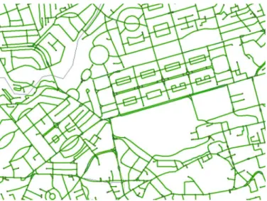
Fig. 1. Part of the road network for Edinburgh (Copyright: Ordnance Survey).

In experiments we used two instances of the city model, each representing a specific city (Edinburgh and Stockholm, respectively). The Edinburgh city model contains approxi-mately 8,750 junctions, 6,800 edges, and 3,300 points of interest. The Stockholm city model contains 7,700 junctions, 3,000 edges, and 1,000 points of interest. Figure 1 shows part of the road network for Edinburgh, including junctions and edges; street names and other information are excluded.

B. Activity recognition

We divide activities into two categories: points of interest and abstract activities. The former includes specific locations that the user may want to visit, while the latter includes general activities such as “look for a restaurant”, “visit a shop”, “go to a bar”, etc. When pursuing a general activity it is assumed that the user is not looking for a specific location, although the user may prefer some locations over others. We also include a special activity associated with ambling, i.e. exploring the city without any particular goal in mind.

For each category, the output of the recognition module is a list of the N most likely activities of that category. Since P(A|O) tends to be very small and it is the relative probabilities that matter, we normalize the output such that the most likely activity A∗

of each category has a score of 100. Each other activityAhas a score of100·P(A|O)/P(A∗

|O). The ranking is simply an ordered list of activities with scores in descending order. For some points of interest we estimated the prior probability from user generated content (details), approximating the “popularity” of each. For the remaining points of interest we assumed a uniform prior distribution.

When using GPS signals, the only relevant information available is the location and direction of the user. We therefore focus on the relevant choices that the user makes with respect to location and direction. Our implementation ignores the user velocity since variation in speed may depend on factors (e.g. user mobility) that are unrelated to the types of activities that we consider. Although different activities may spur the

user to walk at different speeds, it is mainly direction that determines what location or activity the user is interested in.

If the system believes that the user has finished doing an activity, there is a reset mechanism that essentially restarts the system and resets the posterior probabilities of activities according to the prior distribution. In this way, the system has a larger chance of not becoming confused when the user is pursuing several, apparently conflicting, goals. The current reset mechanism is inspired by Pareto’s principle: when the top hypothesis dominates the others by a factor that exceeds a threshold, the system resets itself.

1) Points of Interest: When the goal is to reach a point of interest, we assume that the user has basic knowledge of the location. To reach a point of interest the user would either have to look at a map or ask for directions. If the user has no idea of the location, there is little the recognition module can do to infer the current activity. We can therefore use the city model to estimate the likelihood of going in a certain direction given that the goal is to reach a point of interest.

Due to uncertainty in the GPS signal, it is difficult to observe detailed choices of the pedestrian with respect to location and direction. We therefore focus on four main decisions:

1) Decide which direction to go at a junction.

2) Change direction along an edge of the road network. 3) Decide when to stop at a particular location.

4) Decide when to start walking again.

In each case we take uncertainty into account, e.g. we do not consider that a user has stopped until several seconds have passed, otherwise a noisy GPS signal could lead to false beliefs about the user’s movements.

For each junction j and each point of interest poi, we precompute the optimal distance dist(j, poi) between j and

poialong the road network. Given two neighboring junctions

j and k and a point of interest poi, we define a likelihood

L(k|poi, j) that we use as a substitute for the conditional probabilities P(ai|A, si): the activity is to reach poi, the current junction is j, and the action is to go towards junction

k. We use the optimal distances to estimateL(k|poi, j)as

L(k|poi, j) = dist(j, k) +dist(j, poi)−dist(k, poi) 2·dist(j, k) , where dist(j, k) is the distance between the neighboring junctions j and k. Note that 0 ≤ L(k|poi, j) ≤ 1 since

dist(j, poi)anddist(k, poi)can differ by at mostdist(j, k). A likelihood of0would drive the posterior probabilityP(poi|O) to 0, so we compute an adjusted likelihood Lˆ(k|poi, j) = 0.1 + 0.8 ·L(k|poi, j) such that 0.1 ≤ Lˆ(k|poi, j) ≤ 0.9. Finally, we compute a normalized likelihood as

LN(k|poi, j) =

ˆ

L(k|poi, j)

P

n∈N(j)Lˆ(k|poi, j)

,

where N(j)is the set of all neighboring junctions ofj. Each time the user makes a choice of which direction to go from a given junction, we use the normalized likelihood to update the posterior probability of each activity, i.e. point of interest. This

approach is extended to the case for which the user changes direction along the current edge of the road network.

Before presenting the relative likelihood of different points of interest, we filter the posterior probabilities by a proximity factor, i.e. a probability distribution Φ that considers points of interest in the near proximity as being more likely. The intuition is that although many points of interest may lie in a given direction, locations that are closer are more likely targets. However, we do not want to incorporate the proximity factor into the actual posterior probabilities, which would cause (former) proximity to persist in memory long after the user has left a point of interest behind.

In the case of ambling, we assume that the goal of the user is to visit parts of the city where they have not already been. We compute a normalized likelihoodLN(k|ambling, j) in a similar way toLN(k|poi, j). Going towards intersection

k is more likely if the user has not previously walked along the edge (j, k). Again, the same strategy can be applied when the user changes direction along the current edge. The normalization also makes it possible to compare the posterior probability of ambling with those of points of interest.

When the user stops, we assign a likelihood of0.9to points of interest in the near proximity, and a likelihood of0.1to all other points of interest, including ambling. The intuition is that points of interest in the proximity of the user are likely targets when the user stops. When the user starts walking again, we assign a likelihood of0.9to points of interest not in the vicinity, while the likelihood of nearby points of interest depends on the duration that the user has spent in their vicinity. If the user stopped by chance or due to an erroneous GPS signal, this mechanism will cancel the boost given to points in the vicinity. On the other hand, if the user spent an extended amount of time in the vicinity of a point, it is more likely that the point was a target.

Our system incorporates an optional mode that uses Gaus-sian distributions to model the likelihood of specific points of interest as a function of duration spent in its proximity. The mean and variance of the distribution depends on the type of location. Getting cash from an automatic teller machine is typically much quicker than eating a meal as a restaurant, and these differences are reflected in the distribution. However, it was outside the scope of our project to collect data regarding the duration of different types of activities, so in our system the distributions are manually crafted to reflect our knowledge of different types of points. This is also the reason why the mechanism is optional: our system can incorporate this information if available but will function even when the information is missing. If the optional mode is turned off, all durations are considered equally likely.

An interesting extension of this mechanism would be to take the time of day into consideration when estimating the likelihood of an activity. For example, if a user stops near a restaurant and a bar, the restaurant is a more likely target during lunch hour, but the bar is a more likely target at night. However, estimating this information was again outside the scope of our project.

Fig. 2. Example probability density function for restaurants.

2) General activities: As for general activites, we consider the same four decisions as before. Apart from ambling, we make the assumption that each general activity is associated with a set of points of interest, and that the likelihood of a general activity is proportional to the maximum posterior prob-ability of any point of interest in its associated set. However, just as before, repeatedly incorporating a high likelihood into the posterior probability creates a memory which is difficult to erase. We therefore apply the maximum posterior probability of individual points of interest a posteriori, as a filtering factor, just like the proximity factor for individual points of interest. The only case for which there is a qualitative difference between the likelihood of individual points of interest and that of general activities is when the user starts walking again. Browsing the menu of a restaurant and then leaving should make the probability of that restaurant go down, but the probability of looking for a restaurant in general should go up. The posterior probability of general activities are therefore only updated when the user starts walking again after having stopped. We use the same strategy based on Gaussian distributions over the duration to estimate the likelihood of a given general activity when the user starts walking.

In the case of general activities we can model different

types of events associated with the same point of interest, as shown in Figure 2, which superimposes the likely duration of browsing the menu of a restaurant and the likely duration of having a meal. As seen in the figure, we again adjust the likelihood to a number in the range [0.1,0.9] to avoid multiplication by zero.

C. Familiarity and Visibility

So far, our implementation makes an assumption that the user always knows where they are going, an assumption that

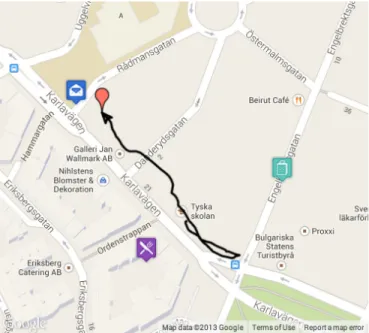
Fig. 3. Example trajectory from the Stockholm city model.

clearly does not always hold, especially if the user is a tourist or visitor. For this reason, the recognition module includes a simple heuristic for estimating how familiar the user is with the surroundings. To compute the heuristic we keep track of the total distance d travelled by the user and compare it to the optimal distanced∗

from the user’s initial location to the current location. We then compute a factorU representing how

unfamiliarthe user is with the surroundings as

U = 1−d

∗

d.

In other words, if the user travelled straight to the current location,U = 0. On the other hand, if the user took a much longer route,U approaches1. Intuitively, the choices that the user makes regarding which direction to go should matter more when we think that the user is familiar with the surroundings. We incorporate familiarity into the conditional probability of walking towards junctionk from junctionj as follows:

(1−U)LN(k|poi, j) +U

1 |N(j)|.

For U = 0, the conditional probability equals LN(k|poi, j), i.e. the same as before. ForU >0, we assign less weight to

LN(k|poi, j) and proportionally more weight to the uniform probability1/|N(j)| (i.e. each neighbor is equally likely).

We also take into account whether a point of interest is

visiblefrom the user’s current location. Intuitively, if the user can see a point of interest, choosing whether or not to go towards it becomes more informative. LetV(poi)be a boolean function that returns1ifpoiis visible from the current junction and0otherwise. We compute an individual unfamiliarity factor for each point of interest as follows:

U(poi) = (1−V(poi))

1−d

∗

d

Fig. 4. Relative ranking of three points of interest.

In other words, the user is considered to be familiar with the location of a point of interest (U(poi) = 0) if they either walked straight to the current location or can see the point. We can now substitute U(poi)forU in the conditional probabilities. We can also generalize this idea and consider intermediate probabilities forV(poi)representing uncertainty.

IV. RESULTS

We ran experiments both in Stockholm and Edinburgh to test the features of the activity recognition module. Figure 3 shows the trajectory of a user in the Stockholm experiments, recorded during earlier work on spoken dialogue systems [11]. The user was told to find a postbox, with no preference for specific targets. The figure shows the postbox eventually found, as well as a restaurant and a shop along the user’s path. Figure 4 shows how the relative ranking for the three particular points of interest in the figure varies over time. For clarity we have excluded many other points of interest in the vicinity. Direction likelihood and proximity filters apply. As we can see, the system initially selects “restaurant” as the top pick, since its one of the nearest targets from the starting point. As the user walks towards the bus stop in the figure, the probability of “restaurant” and “postbox” drops (both due to the proximity filter and the direction likelihood). On the other hand, the probability of “shop” increases slightly. Once the user reaches the bus stop and turns back, the direction likelihood for “restaurant” and “postbox” increases, while that of “shop” remains more or less constant. In this phase we see the effect of proximity filtering. The postbox and the restaurant are in the same direction, but proximity filtering boosts the probability of “restaurant”. Once past the restaurant, the direction likelihood drops rapidly and is compounded by

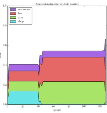
Fig. 5. Relative ranking of general activities.

proximity filtering. As the user closes in on the target (the postbox), the likelihood of this location being the target greatly increases and becomes the top pick of our system.

At the end of the experiment, the system reports the following three points of interest as the top picks:

• restaurant (100) [not shown] • post box (98.58)

• fast food (76.79) [not shown]

Each of these locations has a posterior probability less than 0.07, and there is a very long tail of results, each with a very small posterior probability.

In the experiment we can see how decoupling the direction likelihood from proximity filtering allows our system to be much more responsive. Direction likelihood is aggregated, while filtering is only applied when displaying the results.

The Stockholm experiment includes several other trajecto-ries, but each has few stops, making it difficult to estimate the likelihood of general activities. In another experiment from the Edinburgh city model we simulated a user making two short stops followed by a long one. In the vicinity of the two short stops were an ATM, a restaurant, and a bar. In the vicinity of the long stop were an ATM, a restaurant, and a shop. Figure 5 shows the relative ranking of the four associated general activities over time. After the two short stops, the likelihood of “shop” decreases drastically compared to the others.

Figure 6 shows the ranking of three points along the trajectory: a restaurant near the two short stops (middle), and a restaurant and a shop near the long stop (end). The likelihood of the first restaurant is very high around the time of the two short stops, but then decreases rapidly, unlike the likelihood of the general activity “restaurant” in Figure 5.

Fig. 6. Relative ranking of three points of interest.

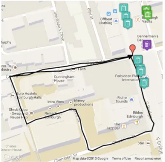
Finally, Figure 7 shows an example trajectory from the Ed-inburgh city model. This experiment was designed to test how familiarity and visibility affects the posterior probability of different targets. The trajectory intentionally describes a loop, simulating a user who is not familiar with the surroundings. We fed the trajectory into the activity recognition module, first with familiarity and visibility turned off, then turned on.

With familiarity and visibility turned off, the points of interest ranked in the top 20 at the end of the trajectory included none that were visible. In contrast, with familiarity and visibility turned on, visible points of interest accounted for 11% of the posterior probability in the top 20.

V. CONCLUSION

We have presented a Bayesian approach to activity recog-nition that estimates the posterior probability of each activity using observations made regarding a user’s behavior. We tested the approach in a city environment where observations were GPS signals indicating the location and direction of users. Our experiments include familiarity and visibility, two concepts that we believe are vital for activity recognition and that we encourage other researchers to explore in future work.

In this work we only consider two types of activities: reaching a specific point of interest, and satisfying a specific type of need (go to a restaurant, purchase an item in a shop, etc.) The flexibility of our Bayesian approach would make it easy to include other types of activities, or more fine-grained activities (e.g. find an Italian restaurant).

ACKNOWLEDGMENT

The authors are grateful for the funding provided by Euro-pean FP7 grant #270019 (SpaceBook).

Fig. 7. Example trajectory from Edinburgh.

REFERENCES

[1] L. Liao, D. Fox, and H. Kautz, “Hierarchical Conditional Random Fields for GPS-based Activity Recognition,” in Robotics Research: The Eleventh International Symposium, Springer Tracts in Advanced Robotics (STAR’07), vol. 28, 2007, pp. 487–506.

[2] G. Andrienko, N. Andrienko, G. Fuchs, A.-M. Olteanu-Raimond, J. Symanzik, and C. Ziemlicki, “Extracting Semantics of Individual Places from Movement Data by Analyzing Temporal Patterns of Visits,” in Proceedings of The First ACM SIGSPATIAL International Workshop on Computational Models of Place (COMP’13), 2013.

[3] D. Ashbrook and T. Starner, “Using GPS to learn significant locations and predict movement across multiple users,” Personal and Ubiquitous Computing, vol. 7, no. 5, pp. 275–286, 2003.

[4] Y. Hu, K. Janowicz, D. Carral, S. Scheider, W. Kuhn, G. Berg-Cross, P. Hitzler, M. Dean, and D. Kolas, “A Geo-ontology Design Pattern for Semantic Trajectories,” in Spatial Information Theory, Lecture Notes in Computer Science (COSIT’13), vol. 8116, 2013, pp. 438–456. [5] L. Alvares, V. Bogorny, B. Kuijpers, J. de Macedo, B. Moelans,

and A. Vaisman, “A model for enriching trajectories with semantic geographical information,” in Proceedings of the ACM International Workshop on Advances in Geographic Information Systems (GIS’07), 2007, pp. 162–169.

[6] A. Palma, V. Bogorny, B. Kuijpers, and L. Alvares, “A clustering-based approach for discovering interesting places in trajectories,” in Proceedings of the ACM Symposium on Applied Computing (SAC’08), 2008, pp. 863–868.

[7] A. Boytsov, A. Zaslavsky, and Z. Abdallah, “Where Have You Been? Using Location Clustering and Context Awareness to Understand Places of Interest,” in Next Generation Teletraffic and Wired/Wireless Advanced Networking, Lecture Notes in Computer Science (NEW2AN’12), vol. 7469, 2012, pp. 51–62.

[8] B. Moreno, V. C. Times, C. Renso, and V. Bogorny, “Looking Inside the Stops of Trajectories of Moving Objects,” in Proceedings of the XI Brazilian Symposium on Geoinformatics (GEOINFO’10), 2010. [9] V. Bogorny, B. Kuijpers, and L. Alvares, “ST-DMQL: A Semantic

Trajectory Data Mining Query Language,” International Journal of Geographical Information Science, vol. 23, no. 10, pp. 1245–1276, 2009. [10] A. Madabhushi and J. Aggarwal, “A Bayesian approach to human activity recognition,” in Proceedings of the 2nd IEEE Workshop on Visual Surveillance (VS’99), 1999, pp. 25–32.

[11] J. Boye, M. Fredriksson, J. G¨otze, J. Gustafson, and J. K¨onigsmann, “Walk this way: Spatial grounding for city exploration,” in Natural Interaction with Robots, Knowbots and Smartphones, 2013, pp. 59–67.