Foundations of Data Science 1

(1)

Foundations of Data Science

1

John Hopcroft

Ravindran Kannan

Version 21/8/2014

These notes are a first draft of a book being written by Hopcroft and Kannan and in many places are incomplete. However, the notes are in good enough shape to prepare lectures for a modern theoretical course in computer science. Please do not put solutions to exercises online as it is important for students to work out solutions for themselves rather than copy them from the internet.

Thanks JEH

(2)

Foundations of Data Science

†

John Hopcroft and Ravindran Kannan

21/8/2014

1 Introduction

Computer science as an academic discipline began in the 60’s. Emphasis was on pro-gramming languages, compilers, operating systems, and the mathematical theory that supported these areas. Courses in theoretical computer science covered finite automata, regular expressions, context free languages, and computability. In the 70’s, algorithms was added as an important component of theory. The emphasis was on making computers useful. Today, a fundamental change is taking place and the focus is more on applications. There are many reasons for this change. The merging of computing and communications has played an important role. The enhanced ability to observe, collect and store data in the natural sciences, in commerce, and in other fields calls for a change in our understand-ing of data and how to handle it in the modern settunderstand-ing. The emergence of the web and social networks, which are by far the largest such structures, presents both opportunities and challenges for theory.

While traditional areas of computer science are still important and highly skilled indi-viduals are needed in these areas, the majority of researchers will be involved with using computers to understand and make usable massive data arising in applications, not just how to make computers useful on specific well-defined problems. With this in mind we have written this book to cover the theory likely to be useful in the next 40 years, just as automata theory, algorithms and related topics gave students an advantage in the last 40 years. One of the major changes is the switch from discrete mathematics to more of an emphasis on probability, statistics, and numerical methods.

Early drafts of the book have been used for both undergraduate and graduate courses. Background material needed for an undergraduate course has been put in the appendix. For this reason, the appendix has homework problems.

This book starts with the treatment of high dimensional geometry. Modern data in diverse fields such as Information Processing, Search, Machine Learning, etc., is often

(8)

represented advantageously as vectors with a large number of components. This is so even in cases when the vector representation is not the natural first choice. Our intuition from two or three dimensional space can be surprisingly off the mark when it comes to high dimensional space. Chapter 2 works out the fundamentals needed to understand the differences. The emphasis of the chapter, as well as the book in general, is to get across the mathematical foundations rather than dwell on particular applications that are only briefly described.

The mathematical areas most relevant to dealing with high-dimensional data are ma-trix algebra and algorithms. We focus on singular value decomposition, a central tool in this area. Chapter 4 gives a from-first-principles description of this. Applications of sin-gular value decomposition include principal component analysis, a widely used technique which we touch upon, as well as modern applications to statistical mixtures of probability densities, discrete optimization, etc., which are described in more detail.

Central to our understanding of large structures, like the web and social networks, is building models to capture essential properties of these structures. The simplest model is that of a random graph formulated by Erd¨os and Renyi, which we study in detail proving that certain global phenomena, like a giant connected component, arise in such structures with only local choices. We also describe other models of random graphs.

One of the surprises of computer science over the last two decades is that some domain-independent methods have been immensely successful in tackling problems from diverse areas. Machine learning is a striking example. We describe the foundations of machine learning, both learning from given training examples, as well as the theory of Vapnik-Chervonenkis dimension, which tells us how many training examples suffice for learning. Another important domain-independent technique is based on Markov chains. The un-derlying mathematical theory, as well as the connections to electrical networks, forms the core of our chapter on Markov chains.

The field of algorithms has traditionally assumed that the input data to a problem is presented in random access memory, which the algorithm can repeatedly access. This is not feasible for modern problems. The streaming model and other models have been formulated to better reflect this. In this setting, sampling plays a crucial role and, indeed, we have to sample on the fly. in Chapter??we study how to draw good samples efficiently and how to estimate statistical, as well as linear algebra quantities, with such samples.

One of the most important tools in the modern toolkit is clustering, dividing data into groups of similar objects. After describing some of the basic methods for clustering, such as the k-means algorithm, we focus on modern developments in understanding these, as well as newer algorithms. The chapter ends with a study of clustering criteria.

(9)

sparse vectors, and compressed sensing. The appendix includes a wealth of background material.

A word about notation in the book. To help the student, we have adopted certain notations, and with a few exceptions, adhered to them. We use lower case letters for scaler variables and functions, bold face lower case for vectors, and upper case letters for matrices. Lower case near the beginning of the alphabet tend to be constants, in the middle of the alphabet, such asi,j, andk,are indices in summations,n andmfor integer sizes, and x, y and z for variables. Where the literature traditionally uses a symbol for a quantity, we also used that symbol, even if it meant abandoning our convention. If we have a set of points in some vector space, and work with a subspace, we use n for the number of points,dfor the dimension of the space, andkfor the dimension of the subspace. The term ”almost surely” means with probability one. We use lnn for the natural logarithm and logn for the base two logarithm. If we want base ten, we will use log₁₀.

To simplify notation and to make it easier to read we useE2₍₁₋_x_{) for} _E₍₁₋_x₎2

and

E(1−x)2 _for _E ₍₁₋_x₎2

(10)

2 High-Dimensional Space

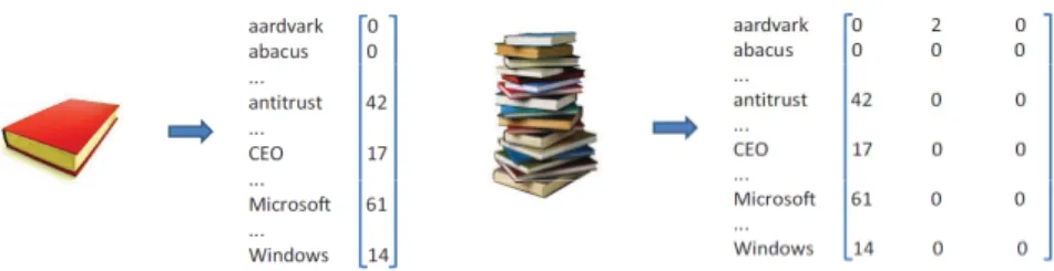
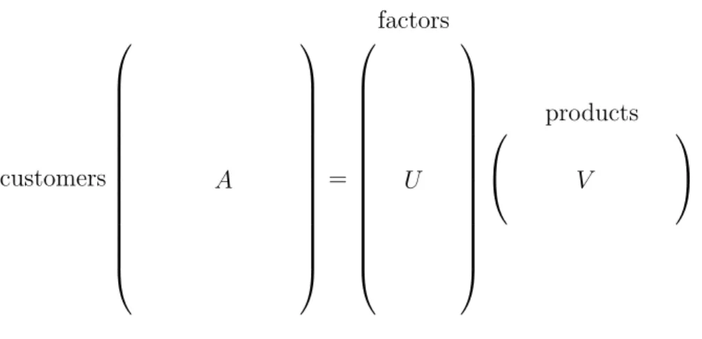
In many applications data is in the form of vectors. In other applications, data is not in the form of vectors, but could be usefully represented by vectors. The Vector Space Model[SWY75] is a good example. In the vector space model, a document is represented by a vector, each component of which corresponds to the number of occurrences of a par-ticular term in the document. The English language has on the order of 25,000 words or terms, so each document is represented by a 25,000 dimensional vector. A collection of n

documents is represented by a collection ofn vectors, one vector per document. The vec-tors may be arranged as columns of a 25,000×n matrix. See Figure 2.1. A query is also represented by a vector in the same space. The component of the vector corresponding to a term in the query, specifies the importance of the term to the query. To find documents about cars that are not race cars, a query vector will have a large positive component for the word car and also for the words engine and perhaps door, and a negative component for the words race, betting, etc.

One needs a measure of relevance or similarity of a query to a document. The dot product or cosine of the angle between the two vectors is an often used measure of sim-ilarity. To respond to a query, one computes the dot product or the cosine of the angle between the query vector and each document vector and returns the documents with the highest values of these quantities. While it is by no means clear that this approach will do well for the information retrieval problem, many empirical studies have established the effectiveness of this general approach.

The vector space model is useful in ranking or ordering a large collection of documents in decreasing order of importance. For large collections, an approach based on human understanding of each document is not feasible. Instead, an automated procedure is needed that is able to rank documents with those central to the collection ranked highest. Each document is represented as a vector with the vectors forming the columns of a matrix

A. The similarity of pairs of documents is defined by the dot product of the vectors. All pairwise similarities are contained in the matrix product AT_A_{. If one assumes that the}

documents central to the collection are those with high similarity to other documents, then computingAT_A _{enables one to create a ranking. Define the total similarity of document}

i to be the sum of the entries in the ith _{row of} _AT_A _{and rank documents by their total}

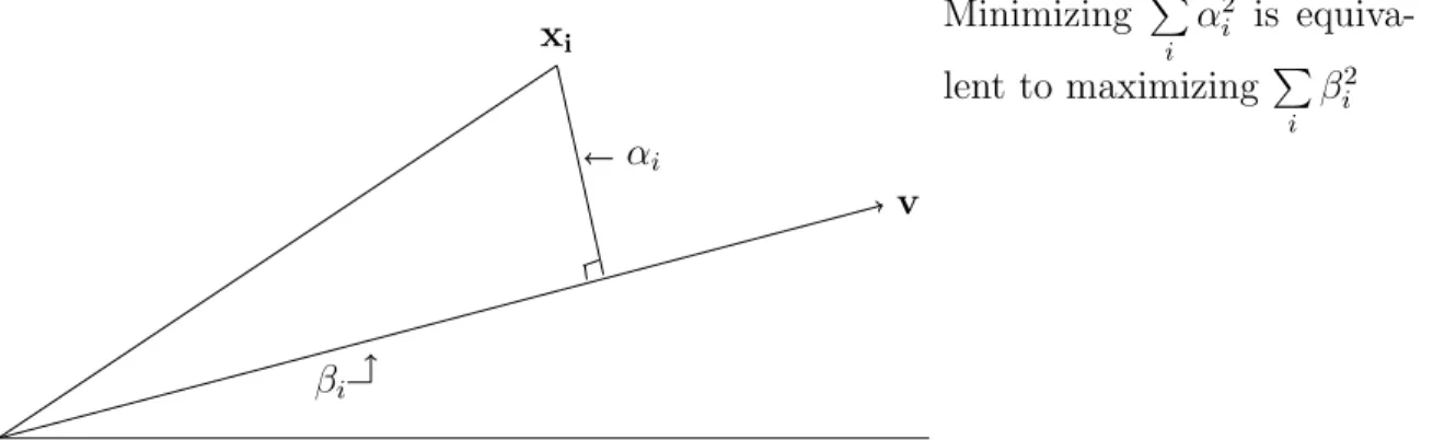
similarity. It turns out that with the vector representation on hand, a better way of ranking is to first find the best fit direction. That is, the unit vectoru,for which the sum of squared perpendicular distances of all the vectors to u is minimized. See Figure 2.2. Then, one ranks the vectors according to their dot product withu. The best-fit direction is a well-studied notion in linear algebra. There is elegant theory and efficient algorithms presented in Chapter 3 that facilitate the ranking as well as applications in many other domains.

(11)

Figure 2.1: A document and its term-document vector along with a collection of docu-ments represented by their term-document vectors.

distance between vectors, and orthogonality, often have natural interpretations and this is what makes the vector representation more important than just a book keeping device. For example, the squared distance between two 0-1 vectors representing links on web pages is the number of web pages linked to by only one of the pages. In Figure 2.3, pages 4 and 5 both have links to pages 1, 3, and 6, but only page 5 has a link to page 2. Thus, the squared distance between the two vectors is one. We have seen that dot products measure similarity. Orthogonality of two nonnegative vectors says that they are disjoint. Thus, if a document collection, e.g., all news articles of a particular year, contained documents on two or more disparate topics, vectors corresponding to documents from different topics would be nearly orthogonal.

The dot product, cosine of the angle, distance, etc., are all measures of similarity or dissimilarity, but there are important mathematical and algorithmic differences between them. The random projection theorem presented in this chapter states that a collection of vectors can be projected to a lower-dimensional space approximately preserving all pairwise distances between vectors. Thus, the nearest neighbors of each vector in the collection can be computed in the projected lower-dimensional space. Such a savings in time is not possible for computing pairwise dot products using a simple projection.

Our aim in this book is to present the reader with the mathematical foundations to deal with high-dimensional data. There are two important parts of this foundation. The first is high-dimensional geometry, along with vectors, matrices, and linear algebra. The second more modern aspect is the combination with probability.

High dimensionality is a common characteristic in many models and for this reason much of this chapter is devoted to the geometry of high-dimensional space, which is quite different from our intuitive understanding of two and three dimensions. We focus first on volumes and surface areas of high-dimensional objects like hyperspheres. We will not present details of any one application, but rather present the fundamental theory useful to many applications.

One reason probability comes in is that many computational problems are hard if our algorithms are required to be efficient on all possible data. In practical situations, domain knowledge often enables the expert to formulate stochastic models of data. In

(12)

best fit line

Figure 2.2: The best fit line is the line that minimizes the sum of the squared perpendicular distances.

web page 4

(1,0,1,0,0,1)

web page 5

(1,1,1,0,0,1)

Figure 2.3: Two web pages as vectors. The squared distance between the two vectors is the number of web pages linked to by just one of the two web pages.

customer-product data, a common assumption is that the goods each customer buys are independent of what goods the others buy. One may also assume that the goods a customer buys satisfies a known probability law, like the Gaussian distribution. In keeping with the spirit of the book, we do not discuss specific stochastic models, but present the fundamentals. An important fundamental is the law of large numbers that states that under the assumption of independence of customers, the total consumption of each good is remarkably close to its mean value. The central limit theorem is of a similar flavor. Indeed, it turns out that picking random points from geometric objects like hyperspheres exhibits almost identical properties in high dimensions. One calls this phenomena the “law of large dimensions”. We will establish these geometric properties first before discussing Chernoff bounds and related theorems on aggregates of independent random variables.

2.1 Properties of High-Dimensional Space

Our intuition about space was formed in two and three dimensions and is often mis-leading in high dimensions. Consider placing 100 points uniformly at random in a unit square. Each coordinate is generated independently and uniformly at random from the interval [0, 1]. Select a point and measure the distance to all other points and observe

(13)

the distribution of distances. Then increase the dimension and generate the points uni-formly at random in a 100-dimensional unit cube. The distribution of distances becomes concentrated about an average distance. The reason is easy to see. Let x and y be two such points ind-dimensions. The distance betweenx and y is

|x−y|=

v u u t

d

X

i=1

(xi−yi)2.

Since Pd

i=1(xi−yi) 2

is the summation of a number of independent random variables of bounded variance, by the law of large numbers the distribution of|x−y|2 _{is concentrated}

about its expected value. Contrast this with the situation where the dimension is two or three and the distribution of distances is spread out.

For another example, consider the difference between picking a point uniformly at random from a unit-radius circle and from a unit-radius sphere in d-dimensions. In d -dimensions the distance from the point to the center of the sphere is very likely to be between 1− c

d and 1, wherec is a constant independent of d. This implies that most of

the mass is near the surface of the sphere. Furthermore, the first coordinate,x1,of such a point is likely to be between−_√c

d and + c

√

d, which we express by saying that most of the

mass is near the equator. The equator perpendicular to thex1 axis is the set {x|x1 = 0}. We will prove these results in this chapter, but first a review of some probability.

2.2 The Law of Large Numbers

In the previous section, we claimed that points generated at random in high dimen-sions were all essentially the same distance apart. The reason is that if one averages

n independent samples x1, x2, . . . , xn of a random variable x, the result will be close to

the expected value ofx. Specifically the probability that the average will differ from the expected value by more than is less than some value _nσ22.

Prob

x1+x2+· · ·+xn

n −E(x)

>

≤ σ

2

n2. (2.1)

Here theσ2 in the numerator is the variance of x. The larger the variance of the random variable, the greater the probability that the error will exceed. The number of points n

is in the denominator since the more values that are averaged, the smaller the probability that the difference will exceed. Similarly the larger is, the smaller the probability that the difference will exceed and hence is in the denominator. Notice that squaring

makes the fraction a dimensionalless quantity.

To prove the law of large numbers we use two inequalities. The first is Markov’s inequality. One can bound the probability that a nonnegative random variable exceedsa

(14)

Theorem 2.1 (Markov’s inequality) Let x be a nonnegative random variable. Then for a >0,

Prob(x≥a)≤ E(x)

a .

Proof: We prove the theorem for continuous random variables. So we use integrals. The same proof works for discrete random variables with sums instead of integrals.

E(x) =

∞ Z

0

xp(x)dx=

a

Z

0

xp(x)dx+

∞ Z

a

xp(x)dx≥

∞ Z

a

xp(x)dx

≥

∞ Z

a

ap(x)dx=a

∞ Z

a

p(x)dx=ap(x≥a)

Thus, Prob(x≥a)≤ E(_ax).

Corollary 2.2 Prob(x≥cE(x))≤ 1

c

Proof: Substitute cE(x) for a.

Markov’s inequality bounds the tail of a distribution using only information about the mean. A tighter bound can be obtained by also using the variance.

Theorem 2.3 (Chebyshev’s inequality)Let x be a random variable with mean m and variance σ2_{. Then}

Prob(|x−m| ≥aσ)≤ 1

a2.

Proof: Prob(|x−m| ≥aσ) = Prob (x−m)2 ≥a2_σ2

. Note that (x−m)2 _{is a} nonneg-ative random variable, so Markov’s inequality can be a applied giving:

Prob (x−m)2 ≥a2σ2≤ E (x−m)

2

a2_σ2 =

σ2

a2_σ2 = 1

a2. Thus, Prob (|x−m| ≥aσ)≤ 1

a2.

The law of large numbers follows from Chebyshev’s inequality. Recall thatE(x+y) =

E(x) +E(y), σ2(cx) =c2σ2(x), σ2(x−m) =σ2(x),and if x and y are independent, then

E(xy) =E(x)E(y) and σ2₍_x₊_y_{) =} _σ2₍_x_{) +}_σ2₍_y₎_. _{To prove} _σ2₍_x₊_y_{) =} _σ2₍_x_{) +}_σ2₍_y₎ when x and y are independent, since σ2₍_x₋_m_{) =} _σ2₍_x₎_, _{one can assume} _E₍_x_{) = 0 and}

E(y) = 0. Thus,

σ2(x+y) =E (x+y)2=E(x2) +E(y2) + 2E(xy) =E(x2) +E(y2) + 2E(x)E(y) =σ2(x) +σ2(y).

(15)

1 1 2 √ 2 2 1 1 2 1 1 1 2 √ d 2

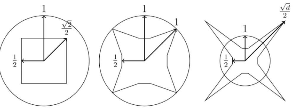
Figure 2.4: Illustration of the relationship between the sphere and the cube in 2, 4, and

d-dimensions.

Theorem 2.4 (Law of large numbers) Let x1, x2, . . . , xn be n samples of a random

variable x. Then

Prob

x1+x2+· · ·+xn

n −E(x)

> ≤ σ 2 n2

Proof: By Chebychev’s inequality

Prob

x1+x2+· · ·+xn

n −E(x)

> ≤ σ

2 x1+x2+···+xn

n

2

≤ 1

n22σ 2₍_x

1 +x2+· · ·+xn)

≤ 1

n22 σ 2₍_x

1) +σ2(x2) +· · ·+σ2(xn)

≤ σ

2₍_x₎

n2 .

The law of large numbers bounds the difference of the sample average and the expected value. Note that the size of the sample for a given error bound is independent of the size of the population class. In the limit, when the sample size goes to infinity, the central limit theorem says that the distribution of the sample average is Gaussian provided the random variable has finite variance. Later, we will consider random variables that are the sum of random variables. That is, x= x1+x2 +· · ·+xn. Chernoff bounds will tell

us about the probability of x differing from its expected value. We will delay this until Section 11.4.11.

2.3 The High-Dimensional Sphere

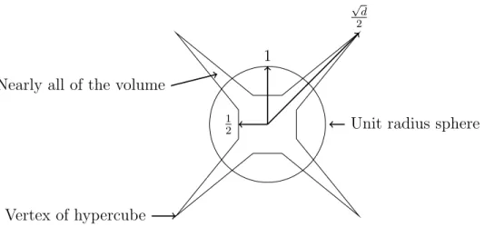
One of the interesting facts about a unit-radius sphere in high dimensions is that as the dimension increases, the volume of the sphere goes to zero. This has important

(16)

1

1 2

√

d

2

Unit radius sphere Nearly all of the volume

Vertex of hypercube

Figure 2.5: Conceptual drawing of a sphere and a cube.

implications. Also, the volume of a high-dimensional sphere is essentially all contained in a thin slice at the equator and simultaneously in a narrow annulus at the surface. There is essentially no interior volume. Similarly, the surface area is essentially all at the equator. These facts, which are contrary to our two or three-dimensional intuition, will be proved by integration.

2.3.1 The Sphere and the Cube in High Dimensions

Consider the difference between the volume of a cube with unit-length sides and the volume of a unit-radius sphere as the dimensiond of the space increases. As the dimen-sion of the cube increases, its volume is always one and the maximum possible distance between two points grows as √d. In contrast, as the dimension of a unit-radius sphere increases, its volume goes to zero and the maximum possible distance between two points stays at two.

For d=2, the unit square centered at the origin lies completely inside the unit-radius circle. The distance from the origin to a vertex of the square is

q

(1 2)

2

+(1₂)2=

√

2

2 ∼= 0.707.

Here, the square lies inside the circle. Atd=4, the distance from the origin to a vertex of a unit cube centered at the origin is

q

(1 2)

2

+₍1₂₎2+₍1₂₎2+₍1₂₎2= 1.

Thus, the vertex lies on the surface of the unit 4-sphere centered at the origin. As the dimension_√ d increases, the distance from the origin to a vertex of the cube increases as

d

2 , and for larged, the vertices of the cube lie far outside the unit radius sphere. Figure 2.5 illustrates conceptually a cube and a sphere. The vertices of the cube are at distance

(17)

Figure 2.6: Volume of sphere in 2 and 3 dimensions.

√

d

2 from the origin and for largedlie outside the unit sphere. On the other hand, the mid point of each face of the cube is only distance 1/2 from the origin and thus is inside the sphere. For large d, almost all the volume of the cube is located outside the sphere.

2.3.2 Volume and Surface Area of the Unit Sphere

For fixed dimension d, the volume of a sphere is a function of its radius and grows as

rd_{. For fixed radius, the volume of a sphere is a function of the dimension of the space.}

What is interesting is that the volume of a unit sphere goes to zero as the dimension of the sphere increases.

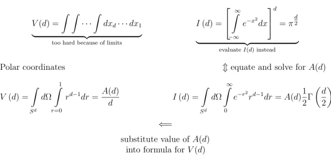
To calculate the volume of a unit-radius sphere, one can integrate in either Cartesian or polar coordinates. In Cartesian coordinates the volume of a unit sphere is given by

V (d) =

x1=1

Z

x1=−1

x2=

√

1−x2 1

Z

x2=−

√

1−x2 1

· · · xd=

√

1−x2

1−···−x2d−1

Z

xd=−

√

1−x2

1−···−x2d−1

dxd· · ·dx2dx1.

Since the limits of the integrals are complicated, it is easier to integrate using polar coordinates. First, lets work out what happens in polar coordinates ford= 2 and d= 3. [See Figure (2.6).] If d = 2, the volume is really the area (which we know to be π). Consider a infinitesimal radial triangle with the origin as the apex. The area between r

and r+dr of this triangle is bounded by two parallel arcs and two radial lines and since the (infinitesimal) arcs are perpendicular to the radius, the area of this piece is justdΩdr, where, dΩ is the arc length. In three dimensions,dΩ is the area (2-dimensional volume) and again, the surface ofdΩ is perpendicular to the radial direction, so the volume of the piece isdΩdr.

In polar coordinates,V(d) is given by

V (d) =

Z

Sd

1

Z

r=0

rd−1drdΩ.

Here, dΩ is the surface area of the infinitesimal piece of the solid angle Sd of the unit sphere. See Figure 2.7. The convex hull of the dΩ piece and the origin form a cone. At radius r, the surface area of the top of the cone is rd−1_d_{Ω since the surface area is} _d₋₁ dimensional and each dimension scales byr. The volume of the infinitesimal piece is base times height, and since the surface of the sphere is perpendicular to the radial direction at each point, the height isdr giving the above integral.

(18)

rdr

dΩ rd−1_d_Ω

dr

Figure 2.7: Infinitesimal volume in a d-dimensional sphere of unit radius.

Since the variables Ω andr do not interact,

V (d) =

Z

Sd

dΩ 1

Z

r=0

rd−1dr= 1

d

Z

Sd

dΩ = A(d)

d

where A(d) is the surface area of a d-dimensional unit-radius sphere. The question re-mains, how to determine the surface area A(d) = R

Sd

dΩ.

Consider a different integral

I(d) =

∞ Z

−∞ ∞ Z

−∞

· · ·

∞ Z

−∞

e−(x21+x22+···x2d)dx

d· · ·dx2dx1.

Including the exponential allows integration to infinity rather than stopping at the surface of the sphere. Thus, I(d) can be computed by integrating in both Cartesian and polar coordinates. Integrating in polar coordinates will relate I(d) to the surface area A(d). Equating the two results forI(d) allows one to solve forA(d).

First, calculate I(d) by integration in Cartesian coordinates.

I(d) =

 

∞ Z

−∞

e−x2dx

 

d

= √πd =πd2_.

Here, we have used the fact that R_−∞∞ e−x2 dx =√π. For a proof of this, see Section ??

of the appendix. Next, calculateI(d) by integrating in polar coordinates. The volume of the differential element isrd−1dΩdr. Thus,

I(d) =

Z

Sd

dΩ

∞ Z

0

(19)

Cartesian coordinates

V(d) =

Z Z

· · ·

Z

dxd· · ·dx1

| {z }

too hard because of limits

I(d) =

 

∞ Z

−∞

e−x2dx

 

d

=πd2

| {z }

evaluateI(d) instead

Polar coordinates mequate and solve for A(d)

V (d) =

Z Sd dΩ 1 Z r=0

rd−1dr = A(d)

d I(d) =

Z Sd dΩ ∞ Z 0

e−r2rd−1dr=A(d)1 2Γ d 2 ⇐=

substitute value ofA(d) into formula for V(d)

Equate integrals for I(d) in Cartesian and polar coordinates and solve for A(d).

Substitute A(d) into the formula for volume of the sphere obtained by integrating in polar coordinates. This gives the result forV(d).

Figure 2.8: Strategy for calculating the volume of a d-dimensional sphere.

The integral R

Sd

dΩ is the integral over the entire solid angle and gives the surface area,

A(d), of a unit sphere. Thus, I(d) = A(d)

∞ R

0

e−r2rd−1dr. Evaluating the remaining integral gives

∞ Z

0

e−r2rd−1dr = 1 2

∞ Z

0

e−ttd2 −1_dt₌ 1 2Γ

d

2

and hence, I(d) =A(d)1₂Γ d₂ where the gamma function Γ (x) is a generalization of the factorial function for noninteger values of x. Γ (x) = (x−1) Γ (x−1), Γ (1) = Γ (2) = 1, and Γ 1₂=√π. For integer x, Γ (x) = (x−1)!.

Combining I(d) = πd2 _with _I₍_d_{) =} _A₍_d₎1 2Γ

d

2

yields

A(d) = π

d 2 1 2Γ d 2

establishing the following lemma.

(20)

dimensions are given by

A(d) = 2π

d

2

Γ d₂ and V (d) = 2

d πd2

Γ d₂.

To check the formula for the volume of a unit sphere, note that V (2) = π and

V (3) = 2₃ π

3 2

Γ(3₂) = 4

3π, which are the correct volumes for the unit spheres in two and three dimensions. To check the formula for the surface area of a unit sphere, note that

A(2) = 2π and A(3) = 2π

3 2 1 2

√

π = 4π, which are the correct surface areas for the unit sphere

in two and three dimensions. Note thatπd2 is an exponential in d

2 and Γ

d

2

grows as the factorial of d₂. This implies that lim

d→∞V(d) = 0, as claimed.

The volume of a d-dimensional sphere of radius r grows as rd. This follows since the unit sphere can be mapped to a sphere of radius r by the linear transformation specified by a diagonal matrix with diagonal elementsr. The determinant of this matrix isrd_. _See

Section 2.4. Since the surface area is the derivative of the volume, the surface area grows asrd−1_. _{See last paragraph of Section 2.3.5.}

The proof of Lemma 2.5 illustrates the relationship between the surface area of the sphere and the Gaussian probability density

1

√

2πe

−(x1+x2+···+xd)2/2_.

This relationship is an important one and will be used several times in this chapter.

2.3.3 The Volume is Near the Equator

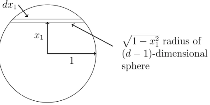
Consider a high-dimensional unit-radius sphere and fix the North Pole on thex1 axis at x1 = 1. Divide the sphere in half by intersecting it with the plane x1 = 0. The intersection of the plane with the sphere forms a region of one lower dimension, namely

x|x| ≤1, x₁ = 0 ,called the equator. The intersection is a sphere of dimension d−1

and has volume V (d−1). In three dimensions this region is a circle, in four dimensions the region is a 3-dimensional sphere, etc. In our terminology, a circle is a 2-dimensional sphere and its volume is what one usually refers to as the area of a circle. The surface area of the 2-dimensional sphere is what one usually refers to as the circumference of a circle.

It turns out that essentially all of the volume of the upper hemisphere lies between the plane x1 = 0 and a parallel plane, x1 = ε, that is slightly higher. For what value of

ε does essentially all the volume lie between x1 = 0 and x1 = ε? The answer depends on the dimension. For dimension d, it is O(_√1

d−1). Before we prove this, some intuition is in order. Since |x|2 ₌ _x2

1+x22 +· · ·+x2d and by symmetry, we expect the x2i ’s to be

generally equal (or close to each other), we expect eachx2

(21)

1

x1

dx1

p

1−x2

1 radius of (d−1)-dimensional sphere

Figure 2.9: The volume of a cross-sectional slab of a d-dimensional sphere.

the proof, we compute the ratio of the volume above the slice lying between x1 = 0 and

x1 = and the volume of the entire upper hemisphere. Actually we compute the ratio of an upper bound on the volume above the slice and a lower bound on the volume of the entire hemisphere and show that this ratio is very small when is Ω(√1

d−1). Volume above slice

Volume upper hemisphere ≤

Upper bound on volume above slice Lower bound on volume upper hemisphere LetT =

x|x| ≤1, x1 ≥ε be the portion of the sphere above the slice. To calculate the volume ofT, integrate overx1 fromε to 1. The incremental volume is a disk of width

dx1whose face is a (d−1)-dimensional sphere of radius

p

1−x2

1.See Figure 2.9. Therefore, the surface area of the disk is

1−x2₁

d−1

2 _V ₍_d₋₁₎

and

Volume (T) = 1

Z

ε

1−x2₁

d−1

2 _V ₍_d₋₁₎_dx

1 =V (d−1) 1

Z

ε

1−x2₁

d−1 2 _dx

1.

Note thatV (d) denotes the volume of the d-dimensional unit sphere. For the volume of other sets such as the set T, we use the notation Volume(T) for the volume.

The above integral is difficult to evaluate, so we use some approximations. First, we use the inequality 1 +x ≤ex _{for all real} _x _{and change the upper bound on the integral}

to infinity. Since x1 is always greater thanε over the region of integration, we can insert

x1/ε in the integral. This gives

Volume (T)≤V (d−1)

∞ Z

ε

e−d

−1 2 x

2 1_dx

1

≤V(d−1)

∞ Z

ε

x1

ε e

−d−1

2 x 2 1_dx₁_.

(22)

Now,R x1e−

d−1 2 x

2 1 dx

1 =−_d₋1₁e−

d−1 2 x

2

1 and, hence,

Volume (T)≤ 1

ε(d−1)e

−d−1

2 ε 2

V (d−1). (2.2)

The actual volume of the upper hemisphere is exactly 1₂V(d). However, we want the volume in terms of V(d−1) instead of V(d) so we can cancel the V(d−1) in the upper bound of the volume above the slice. We do this by calculating a lower bound on the volume of the entire upper hemisphere. Clearly, the volume of the upper hemisphere is at least the volume between the slabsx1 = 0 and x1 = √_d1₋₁, which is at least the volume of the cylinder of radiusq1− 1

d−1 and height 1

√

d−1.The volume of the cylinder is 1/

√

d−1 times the d−1-dimensional volume of the diskR =nx |x| ≤1;x₁ = √1

d−1

o

. Now R is ad−1-dimensional sphere of radius

q

1− 1

d−1 and so its volume is Volume(R) =V(d−1)

1− 1

d−1

(d−1)/2

.

Using (1−x)a ≥1−ax

Volume(R)≥V(d−1)

1− 1

d−1

d−1 2

= 1

2V(d−1). Thus, the volume of the upper hemisphere is at least ₂√1

d−1V(d−1).

The fraction of the volume above the planex1 =εis upper bounded by the ratio of the upper bound on the volume of the hemisphere above the planex1 =ε to the lower bound on the total volume. This ratio is 2

ε√(d−1)e

−d−1 2 ε

2

which leads to the following lemma.

Lemma 2.6 For any c >0, the fraction of the volume of the unit hemisphere above the plane x1 = √_dc₋₁ is less than 2_ce−c

2_/₂

.

Proof: Substitute _√c

d−1 forε in the above.

For a large constant c, 2_ce−c2/2 _{is small. However, if} _c _{is large relative to} √_d₋₁_, _the band is not narrow. In fact, ifc=√d−1,the band is the entire sphere. The important item to remember is that most of the volume of thed-dimensional unit sphere lies within distance O(1/√d) of the equator. If the sphere is of radius r, then the upper bound on the volume abovex1 = becomes

V(d−1)

Z r

ε

(r2−x2₁)(d−1)/2dx1 =V(d−1)rd−1

Z r

ε

(1−(x2₁/r2))(d−1)/2 ≤V(d−1)rd−1

Z

ε

x1

ε e

−x2

1(d−1)/2r2_dx

(23)

r

0(√r

d)

Figure 2.10: Most of the volume of thed-dimensional sphere of radiusris within distance

O(√r

d) of the equator.

from which we see that the upper bound increases by a factor of rd+1. The lower bound on the volume of the upper hemisphere increases byrd, which results in an upper bound on the fraction above the plane x1 = of

2r √d−1e

−d−1 2

2 r2.

Substituting √cr

d−1 for,results in a bound of 2

ce

−c2

2 .Thus, most of the volume of a radius

r sphere lies within distance O(√r

d) of the equator as shown in Figure 2.10.

For c≥2, the fraction of the volume of the hemisphere above x1 = √_dc₋₁ is less than

e−2 ≈ 0.14 and for c ≥ 4 the fraction is less than ₂1e−8 ≈ 3×10−4. Essentially all the volume of the sphere lies in a narrow band at the equator.

Note that we selected a unit vector in the x1 direction and defined the equator to be the intersection of the sphere with a (d−1)-dimensional plane perpendicular to the unit vector. However, we could have selected an arbitrary point on the surface of the sphere and considered the vector from the center of the sphere to that point and defined the equator using the plane through the center perpendicular to this arbitrary vector. Essentially all the volume of the sphere lies in a narrow band about this equator also.

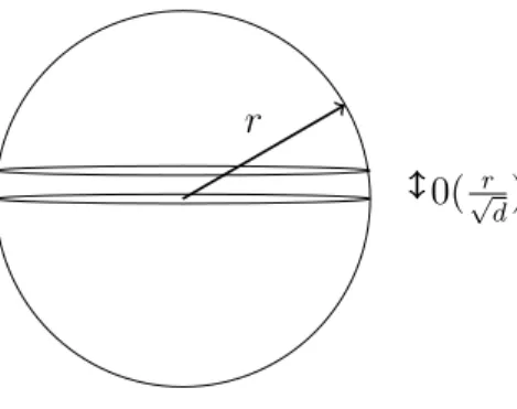
2.3.4 The Volume is in a Narrow Annulus

The ratio of the volume of a sphere of radius 1−ε to the volume of a unit sphere in

d-dimensions is

(1−ε)d_V₍_d₎

V(d) = (1−ε)

d_,

and thus goes to zero asdgoes to infinity when εis a fixed constant. In high dimensions, all of the volume of the sphere is concentrated in a narrow annulus at the surface.

(24)

1 1−

Annulus of width 1_d

Figure 2.11: Most of the volume of the d-dimensional sphere of radius r is contained in an annulus of width O(r/d) near the boundary.

Since, (1−ε)d_≤_e−εd_{, if}_ε₌ c

d, for a large constantc, all bute

−c _{of the volume of the}

sphere is contained in a thin annulus of width c/d. The important item to remember is that most of the volume of the d-dimensional unit sphere is contained in an annulus of widthO(1/d) near the boundary. If the sphere is of radius r, then for sufficiently larged,

the volume is contained in an annulus of widthO r_d.

2.3.5 The Surface Area is Near the Equator

Just as a 2-dimensional circle has an area and a circumference and a 3-dimensional sphere has a volume and a surface area, ad-dimensional sphere has a volume and a surface area. The surface of the sphere is the set x|x|= 1 . The surface of the equator is the

setx|x|= 1, x₁ = 0 and it is the surface of a sphere of one lower dimension, i.e., for a

3-dimensional sphere, it is the circumference of a circle. Just as with volume, essentially all the surface area of a high-dimensional sphere is near the equator. To see this, we use an analogous argument to that used for volume.

First, upper bound the surface area of the sphere abovex1 =ε. LetS =

x|x|= 1, x1 ≥ε . To calculate the surface areaS of the sphere above x1 =ε, integrate x1 fromε to 1. The incremental surface unit will be a band of widthdx1 whose edge is the surface area of a (d−1)-dimensional sphere of radius depending on x1. The radius of the band isp1−x2 1 and therefore, the surface area of the (d−1)-dimensional sphere is

A(d−1) 1−x2₁

d−2 2

whereA(d−1) is the surface area of a unit sphere of dimension d−1. The slice is not a cylinder since whenx1 increases by dx1, the radius r decreases by dr. Thus,

A(S) =A(d−1)

Z 1

(25)

whereds2 ₌_dr2₊_dx2

1. Sincer =

p

1−x2 1, dr=

−x1

√

1−x2 1

dx1 and hence

ds2 =

x2₁

1−x2 1

+ 1

dx2₁ = 1 1−x2

1

dx2₁

and ds= √1 1−x2

1

dx1. Thus,

A(S) =A(d−1)

Z 1

(1−x2₁)d−23dx₁.

The above integral is difficult to integrate and the same approximations, as in the earlier section on volume, lead to the bound

A(S)≤ 1

ε(d−3)e

−d−3

2 ε 2

A(d−1). (2.3)

Next, lower bound the surface area of the entire upper hemisphere. Clearly, the surface area of the upper hemisphere is greater than the surface area of the side of ad-dimensional cylinder of height √1

d−2 and radius

q

1− 1

d−2. The surface area of the cylinder is 1

√

d−2 times the circumference area of the d-dimensional cylinder of radius q1− 1

d−2 which is

A(d−1)(1− 1

d−2)

d−2

2 . Using (1−x)a ≥ 1−ax, the surface area of the hemisphere is at

least

1

√

d−2(1− 1

d−2)

d−2

2 A(d−1)≥ √ 1

d−2(1−

d−2 2

1

d−2)A(d−1)

≥ 1

2√d−2A(d−1). (2.4) Comparing the upper bound on the surface area of S in (2.3) with the lower bound on the surface area of the hemisphere in (2.4), we see that the surface area above the band

x|x|= 1,0≤x₁ ≤ε is less than 4

ε√d−3e

−d−3

2 ε 2

of the total surface area.

Lemma 2.7 For anyc >0, the fraction of the surface area above the plane x1 = √_dc₋₂ is less than or equal to 4_ce−

c2

2 _.

Proof: Substitute √c

d−2 forε in the above.

We conclude this section by relating the surface area and volume of a d-dimensional sphere. So far, we have considered unit-radius spheres of dimension d. Now fix the dimension dand vary the radius r. Let V(d, r) denote the volume and let A(d, r) denote the surface area of a d-dimensional sphere of radius r. Then,

V(d, r) =

Z r

x=0

A(d, x)dx.

Thus, it follows that the surface area is the derivative of the volume with respect to the radius. In two dimensions, the volume of a circle isπr2 _{and the circumference is 2}_πr_{. In} three dimensions, the volume of a sphere is 4₃πr3 and the surface area is 4πr2.

(26)

2.4 Volumes of Other Solids

There are very few high-dimensional solids for which there are closed-form formulae for the volume. The volume of the rectangular solid

R={x|l1 ≤x1 ≤u1, l2 ≤x2 ≤u2, . . . , ld ≤xd≤ud}

is the product of the lengths of its sides. Namely, it is

d

Q

i=1

(ui−li).

A parallelepiped is a solid described by

P ={x|l≤Ax≤u}

where A is an invertible d×d matrix, and l and u are lower and upper bound vectors, respectively. The statements l ≤ Ax and Ax ≤ u are to be interpreted row by row asserting 2d inequalities. A parallelepiped is a generalization of a parallelogram. It is easy to see thatP is the image under an invertible linear transformation of a rectangular solid. Let

R ={y|l≤y≤u}.

The map x=A−1_y _maps _R _to _P_{. This implies that} Volume(P) =Det(A−1)

Volume(R).

Simplices, which are generalizations of triangles, are another class of solids for which volumes can be easily calculated. Consider the triangle in the plane with vertices

{(0,0),(1,0),(1,1)}, which can be described as {(x, y)|0 ≤ y ≤ x ≤ 1}. Its area is 1/2 because two such right triangles can be combined to form the unit square. The generalization is the simplex ind-space with d+ 1 vertices,

{(0,0, . . . ,0),(1,0,0, . . . ,0),(1,1,0,0, . . .0), . . . ,(1,1, . . . ,1)},

which is the set

S ={x|1≥x1 ≥x2 ≥ · · · ≥xd≥0}.

How many copies of this simplex exactly fit into the unit square, {x|0 ≤ xi ≤ 1}?

Every point in the square has some ordering of its coordinates. Since there are d! order-ings, exactly d! simplices fit into the unit square. Thus, the volume of each simplex is 1/d!. Now consider the right angle simplex R whose vertices are the d unit vec-tors (1,0,0, . . . ,0),(0,1,0, . . . ,0), . . . ,(0,0,0, . . . ,0,1) and the origin. A vector y in R

is mapped to an x in S by the mapping: xd = yd; xd−1 = yd +yd−1; . . . ; x1 =

y1 +y2 +· · ·+yd. This is an invertible transformation with determinant one, so the

volume ofR is also 1/d!.

A general simplex is obtained by a translation, adding the same vector to every point, followed by an invertible linear transformation on the right simplex. Convince yourself

(27)

that in the plane every triangle is the image under a translation plus an invertible linear transformation of the right triangle. As in the case of parallelepipeds, applying a linear transformation A multiplies the volume by the determinant of A. Translation does not change the volume. Thus, if the vertices of a simplex T are v1,v2, . . . ,vd+1, then trans-lating the simplex by−vd+1 results in vertices v1−vd+1,v2−vd+1, . . . ,vd−vd+1,0. Let

Abe thed×dmatrix with columns v1−vd+1,v2−vd+1, . . . ,vd−vd+1. Then, A−1T =R and AR=T whereR is the right angle simplex. Thus, the volume of T is _d1_!|Det(A)|.

2.5 Generating Points Uniformly at Random on the Surface of

a Sphere

Consider generating points uniformly at random on the surface of a unit-radius sphere. First, consider the 2-dimensional version of generating points on the circumference of a unit-radius circle by the following method. Independently generate each coordinate uni-formly at random from the interval [−1,1]. This produces points distributed over a square that is large enough to completely contain the unit circle. Project each point onto the unit circle. The distribution is not uniform since more points fall on a line from the origin to a vertex of the square than fall on a line from the origin to the midpoint of an edge of the square due to the difference in length. To solve this problem, discard all points outside the unit circle and project the remaining points onto the circle.

One might generalize this technique in the obvious way to higher dimensions. However, the ratio of the volume of a d-dimensional unit sphere to the volume of a d-dimensional 2 by 2 cube decreases rapidly making the process impractical for high dimensions since almost no points will lie inside the sphere. The solution is to generate a point each of whose coordinates is a Gaussian variable. The probability distribution for a point (x1, x2, . . . , xd) is given by

p(x1, x2, . . . , xd) =

1 (2π)d2

e−

x2

1+x22+···+x2d

2

and is spherically symmetric. Normalizing the vector x = (x1, x2, . . . , xd) to a unit

vec-tor gives a distribution that is uniform over the sphere. Note that once the vecvec-tor is normalized, its coordinates are no longer statistically independent.

2.6 Gaussians in High Dimension

A 1-dimensional Gaussian has its mass close to the origin. However, as the dimension is increased something different happens. Thed-dimensional spherical Gaussian with zero mean and varianceσ2 _{has density function}

p(x) = 1

(2π)d/2σdexp

−|₂x_σ|22

(28)

The value of the Gaussian is maximum at the origin, but there is very little volume there. When σ2 = 1, integrating the probability density over a unit sphere centered at the origin yields nearly zero mass since the volume of a unit sphere is negligible. In fact, one needs to increase the radius of the sphere to√d before there is a significant nonzero volume and hence a nonzero probability mass. If one increases the radius beyond √d, the integral ceases to increase, even though the volume increases, since the probability density is dropping off at a much higher rate. The natural scale for the Gaussian is in units of σ√d.

Expected squared distance of a point from the center of a Gaussian

Consider ad-dimensional Gaussian centered at the origin with varianceσ2_{. For a point}

x= (x1, x2, . . . , xd) chosen at random from the Gaussian, the expected squared length of

xis

E x2₁+x2₂+· · ·+x2_d

=d E x2₁

=dσ2.

For larged, the value of the squared length ofxis tightly concentrated about its mean and thus, althoughE(x2)6=E2(x), E(x)≈pE(x2₎_. _{We call the square root of the expected} squared distance σ√d the radius of the Gaussian. In the rest of this section, we consider spherical Gaussians withσ = 1. All results can be scaled up by σ.

The probability mass of a unit-variance Gaussian as a function of the distance from its center is given by rd−1_e−r2/2 _{times some constant normalization factor where} _r _{is the} distance from the center and d is the dimension of the space. The probability mass function has its maximum at

r=√d−1,

which can be seen from setting the derivative equal to zero.

∂ ∂rr

d−1_e−r

2

2 _{= (}_d−₁₎_rd−2_e−

r2

2 −_rd_e−

r2

2 _{= 0} Dividing byrd−2_e−r2

2 , yields r2 =d−1.

Width of the annulus

The Gaussian distribution in high dimensions, centered at the origin, has its maxi-mum value at the origin. However, there is no probability mass in a sphere of radius one centered at the origin since the sphere has zero volume. In fact, there is no probability mass until one gets sufficiently far from the origin so a sphere of that radius has nonzero volume. This occurs at radius √d. Once one gets a little farther from the origin there is again no probability mass since the probability distribution is dropping exponentially fast and the volume of the sphere is only increasing polynomially fast. All the probability mass is in a narrow annulus of radius approximately √d. In Section 2.7 we prove that for any positive real number β <√d, all but 3e−cβ2

of the mass lies within the annulus

√

(29)

Separating Gaussians

Gaussians are often used to model data. A common stochastic model is the mixture model where one hypothesizes that the data is generated from a convex combination of simple probability densities. An example is two Gaussian densitiesp1(x) andp2(x) where data is drawn from the mixture p(x) = w1p1(x) +w2p2(x) with positive weights w1 and

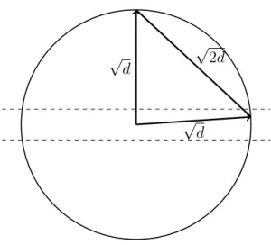
w2 summing to one. Assume that p1 and p2 are spherical with unit variance. If their means are very close, then given data from the mixture, one cannot tell for each data point whether it came from p1 or p2. The question arises as to how much separation is needed between the means to determine which Gaussian generated which data point. We will see that a separation of Ω(d1/4_{) suffices. The algorithm to separate two Gaussians is} simple. Calculate the distance between all pairs of points. Points whose distance apart is smaller are from the same Gaussian, points whose distance is larger are from different Gaussians. Later, we will see that with more sophisticated algorithms, even a separation of Ω(1) suffices.

Consider two spherical unit-variance Gaussians. From Theorem 2.10, most of the probability mass of each Gaussian lies on an annulus of widthO(1) at radius√d−1. Also

e−|x|2/2 =Q

ie

−x2

i/2 and almost all of the mass is within the slab {x| −c≤x

1 ≤c},for

c∈O(1). Pick a point x from the first Gaussian. After picking x, rotate the coordinate system to make the first axis point towards x. Independently pick a second point y also from the first Gaussian. The fact that almost all of the mass of the Gaussian is within the slab {x | −c ≤ x1 ≤ c, c ∈ O(1)} at the equator implies that y’s component along

x’s direction is O(1) with high probability. Thus, y is nearly perpendicular to x. So,

|x− y| ≈ p|x|2₊_|_y_|2_{. See Figure 2.12. More precisely, since the coordinate system} has been rotated so that x is at the North Pole, x = (√d±O(1),0, . . . ,0). Since y is almost on the equator, further rotate the coordinate system so that the component of

y that is perpendicular to the axis of the North Pole is in the second coordinate. Then

y= (O(1),√d±O(1),0, . . . ,0). Thus,

(x−y)2 =d±O(√d) +d±O(√d) = 2d±O(√d) and |x−y|=√2d±O(1).

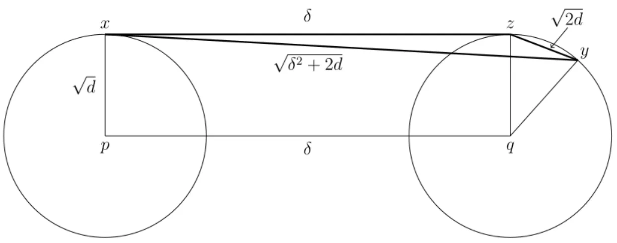
Given two spherical unit variance Gaussians with centers p and q separated by a distanceδ, the distance between a randomly chosen point x from the first Gaussian and a randomly chosen point y from the second is close to √δ2_{+ 2}_d_{, since}_x₋_p_,_p₋_q_, _and

q−y are nearly mutually perpendicular. Pick x and rotate the coordinate system so that x is at the North Pole. Let z be the North Pole of the sphere approximating the second Gaussian. Now pick y. Most of the mass of the second Gaussian is within O(1) of the equator perpendicular to q−z. Also, most of the mass of each Gaussian is within distanceO(1) of the respective equators perpendicular to the line q−p. See Figure 2.13.

(30)

√

d

√

d

√

2d

Figure 2.12: Two randomly chosen points in high dimension are almost surely nearly orthogonal.

Thus,

|x−y|2 _≈_δ2₊_|_z₋_q_|2₊_|_q₋_y_|2 =δ2+ 2d±O(√d)).

To ensure that the distance between two points picked from the same Gaussian are closer to each other than two points picked from different Gaussians requires that the upper limit of the distance between a pair of points from the same Gaussian is at most the lower limit of distance between points from different Gaussians. This requires that

√

2d+O(1) ≤√2d+δ2₋_O_{(1) or 2}_d₊_O₍√_d₎_≤₂_d₊_δ2_{, which holds when} _δ _∈_Ω(_d1/4_). Thus, mixtures of spherical Gaussians can be separated, provided their centers are sepa-rated by more thand14. One can actually separate Gaussians where the centers are much

closer. Chapter 4 contains an algorithm that separates a mixture ofkspherical Gaussians whose centers are much closer.

Algorithm for separating points from two Gaussians

Calculate all pairwise distances between points. The cluster of smallest pairwise distances must come from a single Gaussian. Remove these points. The remaining points come from the second Gaussian.

Fitting a single spherical Gaussian to data

Given a set of sample points, x1,x2, . . . ,xn, in a d-dimensional space, we wish to find the spherical Gaussian that best fits the points. Let F be the unknown Gaussian with

(31)

√

d

δ

p q

x z

y

√

δ2_{+ 2}_d

δ √₂_d

Figure 2.13: Distance between a pair of random points from two different unit spheres approximating the annuli of two Gaussians.

mean µ and variance σ2 _{in each direction. The probability of picking these points when} sampling according toF is given by

cexp − (x1 −µ)

2

+ (x2−µ)

2

+· · ·+ (xn−µ)

2 2σ2

!

where the normalizing constant c is the reciprocal of

R

e−|x−µ|

2 2σ2 dx

n

. In integrating from

−∞ to ∞, one could shift the origin to µ and thus c is

R

e−|x|

2 2σ2dx

−n

= 1

(2π)n2 and is

independent ofµ.

The Maximum Likelihood Estimator (MLE) ofF, given the samplesx1,x2, . . . ,xn, is

the F that maximizes the above probability.

Lemma 2.8 Let {x1,x2, . . . ,xn} be a set of n points in d-space. Then (x1−µ)2 + (x2−µ)2+· · ·+(xn−µ)2 is minimized whenµis the centroid of the pointsx1,x2, . . . ,xn,

namely µ= _n1(x1+x2+· · ·+xn).

Proof: Setting the gradient of (x1−µ)2+ (x2−µ)2+· · ·+ (xn−µ)2 with respectµto

zero yields

−2 (x1−µ)−2 (x2−µ)− · · · −2 (xn−µ) = 0.

Solving forµ gives µ= _n1(x1+x2+· · ·+xn).

To determine the maximum likelihood estimate ofσ2 _for_F_{, set}_µ_{to the true centroid.} Next, we show that σ is set to the standard deviation of the sample. Substitute ν = ₂_σ12

(32)

and a = (x1−µ) 2

+ (x2 −µ) 2

+· · ·+ (xn−µ)

2

into the formula for the probability of picking the pointsx1,x2, . . . ,xn. This gives

e−aν

R

x

e−x2_ν

dx

n .

Now,a is fixed and ν is to be determined. Taking logs, the expression to maximize is

−aν−nln

  Z

x

e−νx2dx

 .

To find the maximum, differentiate with respect toν, set the derivative to zero, and solve forσ. The derivative is

−a+n

R

x

|x|2_e−νx2_dx

R

x

e−νx2

dx .

Settingy=|√νx| in the derivative, yields

−a+ n

ν

R

y

y2e−y2dy

R

y

e−y2

dy .

Since the ratio of the two integrals is the expected distance squared of a d-dimensional spherical Gaussian of standard deviation √1

2 to its center, and this is known to be

d

2, we get −a+ nd₂_ν. Substituting σ2 _for 1

2ν gives −a+ndσ

2_. _Setting₋_a₊_ndσ2 _{= 0 shows that} the maximum occurs when σ =

√

a

√

nd. Note that this quantity is the square root of the

average coordinate distance squared of the samples to their mean, which is the standard deviation of the sample. Thus, we get the following lemma.

Lemma 2.9 The maximum likelihood spherical Gaussian for a set of samples is the one with center equal to the sample mean and standard deviation equal to the standard devia-tion of the sample from the true mean.

Let x1,x2, . . . ,xn be a sample of points generated by a Gaussian probability

distri-bution. µ = 1

n(x1 +x2+· · ·+xn) is an unbiased estimator of the expected value of

the distribution. However, if in estimating the variance from the sample set, we use the estimate of the expected value rather than the true expected value, we will not get an unbiased estimate of the variance, since the sample mean is not independent of the sam-ple set. One should useµ = _n₋1₁(x1+x2+· · ·+xn) when estimating the variance. See

(33)

2.7 Bounds on Tail Probability

Markov’s inequality bounds the tail probability of a nonnegative random variable x

based only on its expectation. For a >0,

Prob(x > a)≤ E(x)

a .

As a grows, the bound drops off as 1/a. Given the second moment of x, Chebyshev’s inequality, which does not assumexis a nonnegative random variable, gives a tail bound falling off as 1/a2

Prob(|x−E(x)| ≥a)≤

E x−E(x)2

a2 .

Higher moments yield bounds by applying either of these two theorems. For example, ifris a nonnegative even integer, thenxr is a nonnegative random variable even ifxtakes on negative values. Applying Markov’s inequality toxr_,

Prob(|x| ≥a) = Prob(xr ≥ar)≤ E(x r₎

ar ,

a bound that falls off as 1/ar_{. The larger the} _r_{, the greater the rate of fall, but a bound}

onE(xr_{) is needed to apply this technique.}

For a random variable x that is the sum of a large number of independent random variables,x1, x2, . . . , xn, one can derive bounds onE(xr) for high evenr. There are many

situations where the sum of a large number of independent random variables arises. For example,xi may be the amount of a good that theith consumer buys, the length of theith

message sent over a network, or the indicator random variable of whether the ith _record

in a large database has a certain property. Each xi is modeled by a simple probability

distribution. Gaussian, exponential (probability density at any t >0 is e−t_{), or binomial}

distributions are typically used, in fact, respectively in the three examples here. If thexi

have 0-1 distributions, there are a number of theorems called Chernoff bounds, bounding the tails of x =x1 +x2 +· · ·+xn, typically proved by the so-called moment-generating

function method (see Section 11.4.11 of the appendix). But exponential and Gaussian ran-dom variables are not bounded and these methods do not apply. However, good bounds on the moments of these two distributions are known. Indeed, for any integer s >0, the

sth _{moment for the unit variance Gaussian and the exponential are both at most} _s_!.

Given bounds on the moments of individual xi the following theorem proves moment

bounds on their sum. We use this theorem to derive tail bounds not only for sums of 0-1 random variables, but also Gaussians, exponentials, Poisson, etc.

The gold standard for tail bounds is the central limit theorem for independent, iden-tically distributed random variablesx1, x2,· · · , xn with zero mean and Var(xi) =σ2 that