M E T H O D O L O G Y
Open Access
Cross-validation pitfalls when selecting and
assessing regression and classification models
Damjan Krstajic
1,2,3*, Ljubomir J Buturovic
3, David E Leahy
4and Simon Thomas
5Abstract
Background:We address the problem of selecting and assessing classification and regression models using cross-validation. Current state-of-the-art methods can yield models with high variance, rendering them unsuitable for a number of practical applications including QSAR. In this paper we describe and evaluate best practices which improve reliability and increase confidence in selected models. A key operational component of the proposed methods is cloud computing which enables routine use of previously infeasible approaches.
Methods:We describe in detail an algorithm for repeated grid-search V-fold cross-validation for parameter tuning in classification and regression, and we define a repeated nested cross-validation algorithm for model assessment. As regards variable selection and parameter tuning we define two algorithms (repeated grid-search cross-validation and double cross-validation), and provide arguments for using the repeated grid-search in the general case.
Results:We show results of our algorithms on seven QSAR datasets. The variation of the prediction performance, which is the result of choosing different splits of the dataset in V-fold cross-validation, needs to be taken into account when selecting and assessing classification and regression models.
Conclusions:We demonstrate the importance of repeating cross-validation when selecting an optimal model, as well as the importance of repeating nested cross-validation when assessing a prediction error.
Background
Allen [1], Stone [2] and Geisser [3], independently intro-duced cross-validation as a way of estimating parameters for predictive models in order to improve predictions. Allen [1] proposed the PRESS (Prediction Sum of Squares) criteria, equivalent to leave-one-out cross-validation, for problems with selection of predictors and suggested it for general use. Stone [2] suggested the use of leave-one-out cross-validation for estimating model parameters and for assessing their predictive error. It is important to note that Stone [2] was the first to clearly differentiate between the use of cross-validation to select the model (“cross-validatory choice”) and to assess the model (“cross-validatory assessment”). Geisser [3] intro-duced the Predictive Sample Reuse Method, a method equivalent to V-fold cross-validation, arguing that it
improves predictive performance of the cross-validatory choice, at a cost of introducing pseudo-randomness in the process. Since then, cross-validation, with its dif-ferent varieties, has been investigated extensively and, due to its universality, gained popularity in statistical modelling.
In an ideal situation we would have enough data to train and validate our models (training samples) and have separate data for assessing the quality of our model (test samples). Both training and test samples would need to be sufficiently large and diverse in order to be represenatitive. However such data rich situations are rare in life sciences, including QSAR. A major problem with selection and assessment of models is that we usu-ally only have information from the training samples, and it is therefore not feasible to calculate a test error. However, even though we cannot calculate the test error, it is possible to estimate the expected test error using training samples. It can be shown that the expected test error is the sum of irreducible error, squared bias and variance (Hastie et al. [4] Eq 7.9). Furthermore, Hastie
et al. [4] show the interplay between bias, variance and
* Correspondence:[email protected] 1
Research Centre for Cheminformatics, Jasenova 7, 11030 Beograd, Serbia
2Laboratory for Molecular Biomedicine, Institute of Molecular Genetics and
Genetic Engineering, University of Belgrade, Vojvode Stepe 444a, 11010 Beograd, Serbia
Full list of author information is available at the end of the article
model complexity in detail. Usually, complex models have small bias and large variance, while simple models have large bias and small variance. We are looking for practically useful trade-offs between bias and variance, for example by minimizing the sum of squared bias and variance.
The model selection process does not require exact computation of various models’complexity, which is often impossible, but only their relative ranking, which is usually feasible. Hastie et al. [4] define effective degrees of free-dom and use it as the measure of model complexity. For example, when selecting a model with the k-nearest neigh-bourhood method, we don’t need to know that the effect-ive degrees of freedom isN/k, whereNis the number of samples. However, for the ranking of models, it is required to understand that the number of neighbourskis inversely related to the model complexity.
Hastie et al.[4] devote a whole chapter in their book to various methods of selecting and assessing statistical models. In this paper we are particularly interested in examining the use of cross-validation to select and as-sess classification and regression models. Our aim is to extend their findings and explain them in more detail.
Methodological advances in the last decade or so have shown that certain common methods of selecting and assessing classification and regression models are flawed. We are aware of the following cross-validation pitfalls when selecting and assessing classification and regres-sion models:
Selection of variables prior to, and not within, cross-validation.
Selection of model based on performance of a single cross-validation.
Reporting a cross-validation error as an estimate of error.
Reporting a single nested cross-validation error as an estimate of error.
We demonstrate the effects of the above pitfalls either by providing references or our own results. We then for-mulate cross-validation algorithms for model selection and model assessment in classification and regression settings which avoid the pitfalls, and then show results of applying these methods on QSAR datasets.
The contributions of this paper are as follows. First, we demonstrate the variability of cross-validation results and point out the need for repeated cross-validation. Second, we define repeated cross-validation algorithms for selecting and assessing classification and regression models which deliver robust models and report the asso-ciated performance assessments. Finally, we propose that advances in cloud computing enable the routine use of these methods in statistical learning.
Methods
Repeated cross-validation
In V-fold cross-validation we divide the dataset pseudo randomly into V folds, and a statistical model is refit V times with the cases of each fold withheld in turn from the training set. We analysed the variation in the predic-tion performance that results from choosing a different split of the data. As far as we are aware, the value and importance of repeated cross-validation has not been extensively explored and discussed in the literature partially, we believe, due to the associated computational costs. To quantify the variation, we repeated cross-validation 50 times and estimated the resulting distri-bution of the performance statistics.
Stratified cross-validation
In stratified V-fold cross-validation the output variable is first stratified and the dataset is pseudo randomly split into V folds making sure that each fold contains approxi-mately the same proportion of different strata. Breiman and Spector [5] report no improvement from executing stratified cross-validation in regression settings. Kohavi [6] studied model selection and assessment for classification problems, and he indicates that stratification is generally a good strategy when creating cross-validation folds. Fur-thermore, we need to be careful here, because stratifica-tionde factobreaks the cross-validation heuristics.
With a large number of repeated cross-validations our opinion is that the issue of stratification becomes redun-dant when selecting a model, while for assessing the model it is wise to use stratified cross-validation. We would like to point out that there is no clear consensus regarding the application of stratified cross-validation or any other splitting strategy which takes into account values of the output variable.
Our compromise is not to use stratification for model selection, but to use it for model assessment.
Parameter tuning with repeated grid-search
multi-dimensional grid. The grid-search cross-validation produces cross-validation estimates of performance statis-tics (for example, error rate) for each point in the grid. Dudoit and van der Laan [8] give the asymptotic proof of selecting the tuning parameter with minimal cross-validation error in V-fold cross-cross-validation and, therefore, provide a theoretical basis for this approach. However, the reality is that we work in a non-asymptotic environ-ment and, furthermore, different splits of data between the folds may produce different optimal tuning parame-ters. Consequently, we usedrepeated grid-search
cross-validation where we repeated cross-validation Nexp
times and for each grid point generated Nexp cross-validation errors. The tuning parameter with minimal
mean cross-validation error was then chosen, and we refer to it as the optimal cross-validatory choice for tuning parameter. Algorithm 1 is the repeated grid-search cross-validation algorithm for parameter tuning in classification and regression used in this paper:
Algorithm 1: parameter tuning with repeated grid-search cross-validation
We have a dataset D which consists of N realisations (Y, X1, X2,…, XP) of one output variable Y and variables X1, X2,…, XP. We have at our disposal a regression or classification model building method F with a tuning parameter vector α. We create a grid of K points α1,
α2,…, αK and wish to find the optimal value among them. Model F predicts either categories for classifica-tion or numbers for regression. We have a loss funcclassifica-tion loss() as a measure of goodness of fit.
1. Repeat the following processNexptimes. a. Divide the dataset D pseudo-randomly into V
folds
b. ForIfrom 1 to V
i. Define set L as the dataset D without theI-th fold
ii. Define set T as theI-th fold of the dataset D iii. Forkfrom 1 to K
1. Build a statistical model fk= f(L;αk) 2. Apply fkon T and store the predictions. c. For eachαvalue calculate the goodness of fit
(loss()) for all elements in D.
2. For eachαvalue calculate the mean of theNexp
calculations of losses.
3. Letα’be theαvalue for which the average loss is minimal. If there are multipleαvalues for which the average loss is minimal, thenα’is the one with the lowest model complexity.
4. Selectα’as the optimal cross-validatory choice for tuning parameter and select statistical model f’= f (D;α’) as the optimal cross-validatory chosen model.
Nested cross-validation for model assessment
We analysed cross-validation methods for model assess-ment. As Stone [2] pointed out, cross-validation can be used for model selection and for model assessment, but the two tasks require different cross-validation ap-proaches. Even though the process of model selection is different from the process of model assessment, there has been a tendency to report the cross-validation error found for the optimal model during the model selection as the assessed model performance. Varma and Simon [9] re-port a bias in error estimation when using cross-validation for model selection, and they suggest using “nested cross-validation” as an almost unbiased estimate of the true error. Close examination shows that the “nested cross-validation” defined by Varma and Simon [9] is the same as“cross-validatory assessment of the cross-validatory choice”defined by Stone [2]. Nevertheless, the importance of the paper by Varma and Simon [9] is that they show in practice by how much a validation error of a cross-validatory chosen model can be biased, i.e. too optimistic. Therefore, we applied stratified nested cross-validation to reduce bias of the resulting error rate estimate.
We refer to procedure of selecting optimal cross-validatory chosen model with pre-defined grid, number of folds and number of repeats as thecross-validation proto-col. It is very similar to Stone’s [2] cross-validatory choice, but more specific. Using Stone’s [2] terminology we can say that the nested cross-validation is the cross-validation as-sessment of large-sample performance of a model M chosen by a specific cross-validation protocol P. To em-phasize the fact that the nested cross-validation estimate depends on the cross-validation protocol, we refer to it as theP-estimateof large-sample performance of model M.
We would like to point out that the “wrapper algo-rithm”as defined by Varma and Simon [9] is similar to our cross-validation protocol, although our definition is more specific. The “estimation plan” as defined by Dudoit and van der Laan [8] is almost identical to our cross-validation protocol, the only difference being that we specify repetition.
We also demonstrate that single stratified nested cross-validation errors can vary substantially between different partitionings of the training dataset, and therefore used re-peated stratified nested cross-validation. Algorithm 2 is the general algorithm for repeated stratified nested cross-validation.
Algorithm 2: repeated stratified nested cross-validation
1. Cross-validation protocolPis to useNexp1repeated V1-fold cross-validation with a grid of K pointsα1, α2,…,αK.Designate by M the model chosen by
application of the cross-validation protocolP.
a. Stratify the output variable Y.
b. Divide the dataset D pseudo-randomly into V2 folds making sure that each fold contains the same proportion of each of the Y strata. c. ForIfrom 1 to V2
i. Define set L as the dataset D without theI-th fold
ii. Define set T as theI-th fold of the dataset D iii. Apply the cross-validation protocol to select
model f’, i.e. useNexp1repeated V1-fold cross-validation with a grid of K pointsα1,α2,…,αK
to find an optimal cross-validatory chosen model f’on dataset L.
iv. Apply f’on T
d. Calculate loss() for all elements of D. We refer to it as the nested cross-validation error.
3. The interval between the minimum and maximum ofNexp2nested cross-validation errors is the P-estimated interval of the large-sample error of model M. The mean ofNexp2nested cross-validation errors is the P-estimate of the large-sample error of the model M.
We are not aware of any research finding which suggests that number of folds in the outer cross-validation loop (V2) and number of folds in the inner cross-validation loop (V1) need to be the same or different. Similarly, the number of repeats of the nested cross-validation may or may not be equal to the number of repeats of the cross-validation. We used nested cross-validation with V1 = V2 = 10 and Nexp1 = Nexp2 = 50.
In addition to mean nested cross-validation error we reported the minimum and maximum nested cross-validation errors because the variability is such that reporting a single error value may be misleading.
Variable selection and parameter tuning
The relationship between variable selection and cross-validation was first independently tackled by Allen [1] and Stone [2]. Unfortunately the importance of selecting variables within, and not prior to, cross-validation was widely missed. Ambroise and McLachlan [10] showed how results are biased when selection of variables is done prior to cross-validation. Hastieet al.[4] in chapter 7.10.2 of their book defined the correct way to carry out cross-validation as follows:
1. Divide the samples into K cross-validation folds (groups) at random.
2. For each fold k = 1,2,..,K
a) Find a subset of“good”predictors that show fairly strong (univariate) correlation with the class labels, using all of the samples except those in fold k.
b)Using just this subset of predictors, build a multivariate classifier, using all of the samples except those in fold k.
c) Use the classifier to predict the class labels for the sample in fold k.
The error estimates from step 2(c) are then accumulated over all K folds, to produce the cross-validation estimate of the prediction error.
However, Hastie et al. [4] did not elaborate any fur-ther. As far as we are aware, there are two different ways to implement the above correctly, and we explain each in detail below.
When selecting variables and parameter tuning, our goal is to select the optimal number of variables and the optimal parameter values. Here, again, we can view this as a hyper-parameter optimisation problem and apply grid search. Cross-validation would be used for selecting the number of variables (n) and for tuning parameters (α) from a multi-dimensional grid (n,α), where n∈(1, 2,…, P) andα∈(α1,
α2,…,αK). This requires only one cross-validation loop be-cause it treats each point in the multi-dimensional grid independently. We use the same notation as before with an additional variable selection method S, which for the sake of simplicity only takes two input parameters (num-ber of variables to select and the dataset) and returns a new dataset with only the selected variables.
Algorithm 3: repeated grid-search cross-validation for variable selection and parameter tuning
1. Repeat the following processNexptimes.
a. Divide the dataset D pseudo-randomly into V folds b. ForIfrom 1 to V
i. Define set L as the dataset D without theI-th fold ii. Define set T as theI-th fold of the dataset D iii. Forpfrom 1 to P
1. L’= S(L;p); Define set L’as set L with only
pselected variables.
2. Define T’as set T with onlypselected variables as in L’.
3. Forkfrom 1 to K
a. Build a statistical model f’= f(L’;αk) b. Apply f’on T’and store predictions. c. For each point in the grid (n,α) calculate loss()
for all elements of D.
2. For each point in the grid (n,α) calculate average loss. 3. Define the pair (p’,α’) with minimal average loss as
the optimal pair of number of selected variables and parameter values.
4. D’= S(D; p’); define set D’as D with only p’selected predictor variables.
Double cross-validation
Stone [2] suggested an algorithm under the name
“double cross-validation” which involves an additional (internal) cross-validation for parameter tuning for each set of selected variables. As it contains an external and internal validation similar to nested cross-validation, we have found that terms “double cross-validation” and “nested cross-validation” have been used in the literature with different meanings. We use the term “nested cross-validation” as did Varma and Simon [9], meaning the model assessment procedure, and
“double cross-validation”, as did Stone [2], meaning the model selection procedure where variables are selected in addition to parameter tuning. Even though we are not using double cross-validation, we consider it to be important to describe it in our context.
Algorithm 4: double cross-validation
The double cross-validatio algorithm consists of two steps. Step 1. Select number of variables
1. Divide the dataset D pseudo-randomly into V1 folds
2. ForIfrom 1 to V1
a. Define set L as the dataset D without theI-th fold
b. Define set T as theI-th fold of the dataset D c. Forpfrom 1 to P
i. L’= S(L;p); Define set L’as set L with only
pselected predictor variables.
ii. Define T’as set T with onlypselected predictors as in L’.
iii. Divide the dataset L’pseudo-randomly into V2 folds
iv. ForJfrom 1 to V2
1. Define set LL’as the dataset L’withoutJ-th fold
2. Define set TL’as theJ-th fold of the dataset L’
3. Forkfrom 1 to K
a. Build a statistical model f’= f(LL’;αk) b. Apply f’on TL’and store predictions. v. For eachαvalue calculate the loss() for all
elements in L’.
vi. Defineα’asαvalue for which the loss function is minimal.
vii.Build a statistical model f’= f(L’;α’) viii.Apply f’on T and store predictions
3. For each number of selected variables calculate loss () for all elements of D.
4. Define p’as the number of selected variables for which the loss() is minimal.
5. Select p’as the optimal cross-validatory choice of number of selected variables.
Step 2. Select tuning parameter
1. D’= S(D; p’); define set D’as set D with only p’ selected predictor variables.
2. Divide the dataset D’pseudo-randomly into V folds 3. ForIfrom 1 to V
a. Define set L’as the dataset D’withoutI-th fold b. Define set T’as theI-th fold of the dataset D’ c. Forkfrom 1 to K
i. Build a statistical model f’= f(L’;αk) ii. Apply f’on T’and store predictions.
4. For eachαvalue calculate the loss() for all elements in D’
5. Letα’beαvalue for which the loss is minimal. 6. Selectα’as the optimal cross-validatory choice of
tuning parameter and select statistical model f’= f (D’;α’) as the optimal cross-validatory chosen model.
We are not aware of any research that suggests using grid-search in favour of double cross-validation or vice versa. However, in our opinion, double cross-validation as defined above should not be used when parameters used for tuning affect model complexity. For example, if we use a variable selection method and k-nearest neigh-bourhood, then both the number of selected variables and number of neighbours, k, directly affect model com-plexity. Therefore, in step 1 in the external loop we might choose different k for different L’and for a fixed number of variables end up averaging over models with different model complexities. This cannot happen with grid-search cross-validation, because each point in the grid has a fixed number of selected variables and a fixed number of neighbours, k. Furthermore, each point in the grid is treated independently of all others. We used grid-search cross-validation in all experiments.
Pre-processing
The issue of removing variables prior to model build-ing is, however, not without contention. Zhu et al. [11] focus on the bias that arises when a full data set is not available compared to the prediction rule that is formed by working with top-ranked variables from the full set.
Data sets
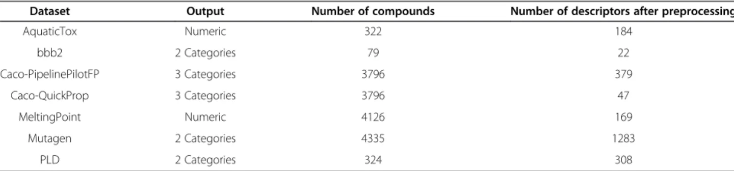
In this section, we report results of applying Algorithms 1–3 on seven QSAR datasets. Table 1 shows the summary of the datasets. Note that in this Section we sometimes use the term “descriptor” instead of“input variable” as is common in QSAR. We have used the following publicly available datasets from the QSARdata R package [12]:
AquaticToxcontains negative log of toxic activity for 322 compounds. It was described and compiled by He and Jurs [13]. The package contains several sets of descriptors for this problem. We chose to use two dimensional MOE descriptors as an example, because when compared to other descriptor sets it generated better models (results not shown). There are 220 MOE 2D descriptors for each compound. However, during pre-processing we removed 30 de-scriptors with near zero variation and 6 dede-scriptors that were linear combinations of others, leaving 184 descriptors for model building.
bbb2contains blood–brain barrier categories (“crossing”or“not crossing”) for 80 compounds from Burns andWeaver [14]. There are 45 compounds categorised as“crossing”and 35 compounds as“not crossing”. The package contains several sets of descriptors for this problem. We chose to use LCALC descriptors as an example, because when compared to other descriptor sets it generated better models (results not shown). We had to remove chloramphenicol from the dataset because LCALC descriptors were not provided for it. There are 23 LCALC descriptors for each compound. During pre-processing we removed descriptor LCALC_NDA as it was a linear combinations of others, leaving 22 descriptors for model building.
cacocontains permeability categories
(“low”,“medium”,“high”) for 3796 compounds from Pham-Theet al.[15]. There are 377 compounds categorised as“low”, 2029 compounds as“medium” and 1390 compounds as“high”. The package contains several sets of descriptors for this problem. As this is the only multi category dataset, we chose to use two sets of descriptors (PipelinePilotFP and QuickProp), because when compared to other descriptor sets they generated better models (results not shown). There are 5401 PipelinePilotFP descriptors for each compound. During pre-processing we removed 4503 descriptors with near zero variation and 519 descriptors that were linear combinations of others, leaving 379 PipelinePilotFP descriptors for model building. There are 51 QuickProp descriptors for each compound. During pre-processing we removed 4 descriptors with near zero variation, leaving 47 QuickProp descriptors for model building. MeltingPointcontaints melting points for 4126
compounds used for model building in Karthikeyan
et al.[16]. In the QSARdata package there is one set of 202 descriptors. During pre-processing we removed 11 descriptors with near zero variation and 22 descriptors that were linear combinations of others, leaving 169 descriptors for model building.
Mutagencontains mutagenicity categories
(“mutagen”or“nonmutagen”) for 4335 compounds from Kaziuset al.[17]. There are 2400 compounds categorised as“mutagen”and 1935 compounds as
“nonmutagen”. In the package there is one set of 1579 descriptors. During pre-processing we removed 281 descriptors with near zero variation and 15 descriptors that were linear combinations of others, leaving 1283 descriptors for model building. PLDcontains phospholipidosis categories (“inducer”
or“noninducer”) for 324 compounds from Goracci
et al.[18].There are 124 compounds categorised as
“inducer”and 200 compounds as“noninducer”. The package comes with several sets of descriptors for this problem. We chose to use PipelinePilotFP,
Table 1 Seven QSAR datasets
Dataset Output Number of compounds Number of descriptors after preprocessing
AquaticTox Numeric 322 184
bbb2 2 Categories 79 22
Caco-PipelinePilotFP 3 Categories 3796 379
Caco-QuickProp 3 Categories 3796 47
MeltingPoint Numeric 4126 169
Mutagen 2 Categories 4335 1283
PLD 2 Categories 324 308
because when compared to other descriptor sets it generated better models (results not shown). There are 2862 PipelinePilotFP descriptors for each compound. During pre-processing we removed 2183 descriptors with near zero variation and 371 descrip-tors that were linear combinations of others, leaving 308 descriptors for model building.
Methods for prediction
In our examples we apply ridge regression and partial-least squares (PLS) on regression problems, while for classification problems we use ridge logistic regression and linear SVM coupled with Pearson’s rank based vari-able selection. We use sum of squared residuals and pro-portion misclassified as the loss functions for regression and classification, respectively.
The process of ranking and selectingP variables using Pearson’s correlation is as follows. The Pearson’s correl-ation coefficient is calculated between each input vari-able Xi and the output varivari-able Y. The absolute values of the coefficients are sorted in descending order and the firstPvariables are selected. The method is quick and in our experience works well with the SVM classification method.
SVM is a widely used technique in solving classification problems. SVM performs classification by constructing an N-dimensional hyper plane that optimally separates the data into two categories. SVM is usually applied in con-junction with a kernel function, which is used to trans-form input data into a higher-dimensional space where the construction of the hyperplane is easier. There are four basic SVM kernels: linear, polynomial, Radial Basis Function (RBF), and sigmoid. For the sake of simplicity we use linear SVM, which requires a parameter C (cost) to be supplied. We searched for the optimal model with values for C of 0.5, 1, 2, 4, 8, and 16. We used the R package e1071 [19] for building SVM models.
Hoerl and Kennard [20] proposed ridge regression, a penalized least squares regression, to achieve better pre-dictions in the presence of multicolinearity of predic-tors. In ridge regression the extent of coefficient shrinkage is determined by one parameter, usually referred to as lambda (λ), and it is inversely related to the model com-plexity. Applying ridge regression tends to improve predic-tion performance but it results in all small, but non-zero, regression coefficients. Friedman et al. [21] developed a fast algorithm for fitting generalised linear models with various penalties, and we used their glmnet R package [22] to apply ridge regression and ridge logistic regression for classification purposes. Typical usage is to let the glmnet function compute its own array of lambda values based on nlambda (number of lambda values–default is 100) and lambda.min.ratio (ratio between the maximum and minimum lambda value). We searched for the
optimal model with nlambda = 100 and lambda.min.ra-tio = 10−6.
PLS was introduced by Wold [23]. The method itera-tively creates components, which are linear combination of input variables, with a goal of maximising variance and correlation with the output variable. The idea is to transform the input space of X1, X2,…, XPvariables into a new hyper plane, with low dimensions, such that coor-dinates of the projections onto this hyper plane are good predictors of the output variable Y. As it is an iterative process, with each newly added component we increase complexity of the model. The method is very popular amongst QSAR modellers due to its simplicity and good results in high-dimensional settings. We searched for the optimal model with a grid of number of components from 1 to 60. We used the R package pls [24] for build-ing PLS models.
Results and experimental Repeated cross-validation
We applied Algorithm1 with Nexp = 50 and V = 10 to the following nine combinations of modelling method and dataset:
1. PLS on AquaticTox
2. Ridge regression on AquaticTox 3. Ridge logistic regression on bbb2
4. Ridge logistic regression on caco-PipelinePilotFP 5. Ridge logistic regression on caco-QuickProp 6. PLS on MeltingPoint
7. Ridge regression on MeltingPoint 8. Ridge logistic regression on Mutagen 9. Ridge logistic regression on PLD
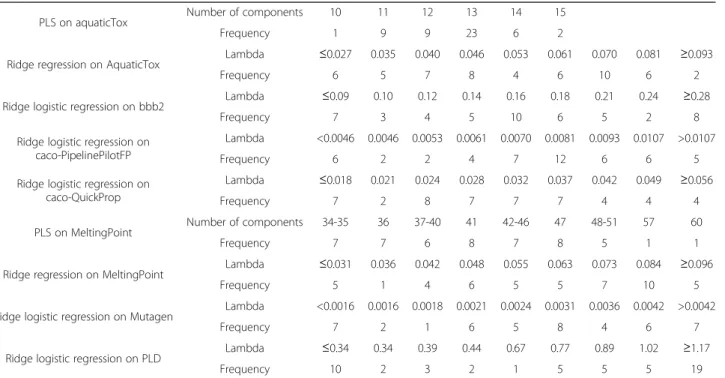
In order to show how the cross-validatory choice of parameter may vary if based on single cross-validation, for all nine cases we found 50 cross-validatory chosen parameters corresponding to 50 single cross-validations. Table 2 shows distributions of optimal cross-validatory chosen parameters for each dataset. It is obvious that the model selected by single cross-validation may have high variance.
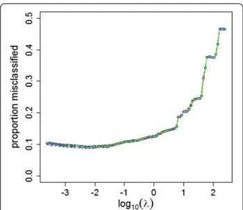
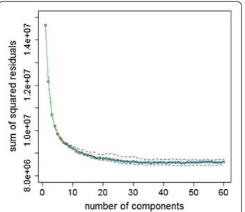
Figures 1, 2, 3, 4, 5, 6, 7, 8 and 9 show for each dataset/ method combination the minimum, first quartile, median, third quartile and maximum cross-validated loss () from 50 repeats as a function of the single hyperparameter.
Nested cross-validation
Our goal is to show examples of nested cross-validation results and its benefits, and not to analyse why one method or set of descriptors performed better than the other.
We applied two linear regressions (PLS and ridge) on AquaticTox (Figure 10) and MeltingPoint (Figure 11). Ridge models on average give slightly better error estimates than PLS models. However, their interval of nested cross-validation error estimates is almost identical. Our conclu-sion would be to use ridge regresconclu-sion for cross-validation on both datasets, but the expected difference between PLS and ridge cross-validatory chosen models are minute.
It is interesting that for caco-PipelinePilotFP nested cross-validation proportions misclassified are almost identi-cal to those for cross-validation, while for caco-QuickProp they are slightly higher (Figure 12). Our conclusion is that if we would to use ridge logistic regression to predict caco and we had to chose between PipelinePilotFP and Quick-Prop descriptors, we would chose PipelinePilotFP.
In the cases of bbb2 (Figure 13), Mutagen (Figure 14) and PLD (Figure 15), where we only performed ridge lo-gistic regression, the interval of nested cross-validation error estimates give us realistic expectations regarding our usage of the cross-validation protocol.
Variable selection and parameter tuning
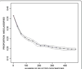
As an example of Algorithm 3, we applied linear SVM coupled with Pearson’s rank based selection on the Mutagen dataset. We searched for the optimal number of descriptors from 1 to 480 with a step size of 30 {1, 30, 60, .. , 450, 480} using linearSVM with the following C
parameters {0.5, 1, 2, 4, 8, 16}. Our grid search consisted of 21 × 6 = 126 points, and we repeated the cross-validation process 50 times. The minimum, mean and maximum cross-validated proportion misclassified from 50 repeats were calculated for all 126 grid points. In order to show results graphically, we selected the cost parameter which generated the lowest mean
cross-Table 2 Distribution of optimal parameters
PLS on aquaticTox Number of components 10 11 12 13 14 15
Frequency 1 9 9 23 6 2
Ridge regression on AquaticTox Lambda ≤0.027 0.035 0.040 0.046 0.053 0.061 0.070 0.081 ≥0.093
Frequency 6 5 7 8 4 6 10 6 2
Ridge logistic regression on bbb2 Lambda ≤0.09 0.10 0.12 0.14 0.16 0.18 0.21 0.24 ≥0.28
Frequency 7 3 4 5 10 6 5 2 8
Ridge logistic regression on caco-PipelinePilotFP
Lambda <0.0046 0.0046 0.0053 0.0061 0.0070 0.0081 0.0093 0.0107 >0.0107
Frequency 6 2 2 4 7 12 6 6 5
Ridge logistic regression on caco-QuickProp
Lambda ≤0.018 0.021 0.024 0.028 0.032 0.037 0.042 0.049 ≥0.056
Frequency 7 2 8 7 7 7 4 4 4
PLS on MeltingPoint Number of components 34-35 36 37-40 41 42-46 47 48-51 57 60
Frequency 7 7 6 8 7 8 5 1 1
Ridge regression on MeltingPoint Lambda ≤0.031 0.036 0.042 0.048 0.055 0.063 0.073 0.084 ≥0.096
Frequency 5 1 4 6 5 5 7 10 5
Ridge logistic regression on Mutagen Lambda <0.0016 0.0016 0.0018 0.0021 0.0024 0.0031 0.0036 0.0042 >0.0042
Frequency 7 2 1 6 5 8 4 6 7
Ridge logistic regression on PLD Lambda ≤0.34 0.34 0.39 0.44 0.67 0.77 0.89 1.02 ≥1.17
Frequency 10 2 3 2 1 5 5 5 19
validation error for each number of selected descriptors. Figure 16 shows the minimum, mean and maximum cross-validated proportion misclassified for every num-ber of selected descriptors. The lowest average cross-validated misclassification error (0.196) is found for n = 450 and C = 8. In other words, this approach selected 450 descriptors, using Pearson’s rank based selection procedure, and linear SVM model with C = 8 as the classifier.
Discussion
We sought to analyse and improve upon the existing cross-validation practices in selection and assessment of regression and classification models. No single cross-validation run provided for reliable selection of the best model on those datasets. Robust model selection required summarising the loss function across multiple repetitions of cross-validation. The model selection behaviour of a
Figure 2Ridge regression on AquaticTox (50 repeats 10 fold CV).Minimum, first quartile, median, third quartile and maximum cross-validated sum of squared residuals from 50 repeats of 10-fold cross-validation of ridge regression on AquaticTox for 100λvalues.
Figure 3Ridge logistic regression on bbb2 (50 repeats 10 fold CV).Minimum, first quartile, median, third quartile and maximum cross-validated proportion misclassified from 50 repeats of 10-fold cross-validation of ridge logistic regression on bbb2 for 100λvalues.
Figure 4Ridge logistic regression on caco-PipelinePilotFP (50 repeats 10 fold CV).Minimum, first quartile, median, third quartile and maximum cross-validated proportion misclassified from 50 repeats of 10-fold cross-validation of ridge logistic regression on caco-PipelinePilotFP for 100λvalues.
particular dataset could only be discerned upon perform-ing the repeated cross-validation. Our model selection was based on average loss.
The nested cross-validation loss estimates differed sig-nificantly compared with the cross-validation estimates of the best model on at least caco-QuickProp, Melting Point Mutagen and PLD datasets. This confirms previ-ous reports in the literature (Varma and Simon [9]).
Model assessment using repeated nested cross-validation (Figures 10, 11, 12, 13, 14 and 15) showed large variation of
loss estimates across the nested cross-validation runs. For example, the proportion misclassified estimate for bbb2 varied between approximately 0.13 and 0.23 (Figure 13). In practical terms, this means that the best model selected on this dataset may have large-sample performance of any-where between 13% and 23%. Whether this is adequate for a particular application is a domain-dependent question, however we point out that the repeated nested cross-validation provides the means to make an informed de-cision regarding the acceptance of the best model.
Figure 6PLS on MeltingPoint (50 repeats 10 fold CV).Minimum, first quartile, median, third quartile and maximum cross-validated sum of squared residuals from 50 repeats of 10-fold cross-validation of PLS on MeltingPoint for number of components from 1 till 60.
Figure 7Ridge regression on MeltingPoint (50 repeats 10 fold CV).Minimum, first quartile, median, third quartile and maximum cross-validated sum of squared residuals from 50 repeats of 10-fold cross-validation of ridge regression on MeltingPoint for 100λvalues.
Figure 8Ridge logistic regression on Mutagen (50 repeats 10 fold CV).Minimum, first quartile, median, third quartile and maximum cross-validated proportion misclassified from 50 repeats of 10-fold cross-validation of ridge logistic regression on Mutagen for 100λvalues.
In all our examples we used 10-fold cross-validation. Kohavi [6] and Hastieet al.[4] empirically show that V-fold validation compared to leave-one-out cross-validation has lower variance, and therefore tends to select simpler models. For some examples we executed 5-fold cross-validation and 5-fold nested cross-validation (results not shown), but did not observe a substantial difference from 10-fold.
Table 3 shows the summary of optimal cross-validatory chosen models for all nine datasets. When reporting the chosen parameter it is important to specify the details of the protocol, i.e. number of folds in cross-validations, the grid width and size, as well as the number of repeats.
We mentioned previously that Dudoit and van der Laan [8] proved the asymptotics of the cross-validatory choice for V-fold cross-validation. However, Breiman
et al. [25] have found in the case of selecting optimal
tree size for classification tree models that the tree size with minimal cross-validation error generates a model which generally overfits. Therefore, in Section 3.4.3 of their book Breiman et al. [25] define the one standard error rule (1 SE rule) for choosing an optimal tree size, and they implement it throughout the book. In order to calculate the standard error for single V-fold cross-validation, accuracy needs to be calculated for each fold, and the standard error is calculated from V accuracies from each fold. Hastie et al. [4] define the 1 SE rule as selecting the most parsimonious model whose error is no more than one standard error above the error of the best model, and they suggest in several places using the 1 SE rule for general cross-validation use. The main point of the 1 SE rule, with which we agree, is to choose the simplest model whose accuracy is comparable with the best model. However, when we repeat cross-validations standard error becomes smaller and the 1 SE rule does not have any effect. We are proposing that
Table 3 Selected optimal cross-validatory chosen models
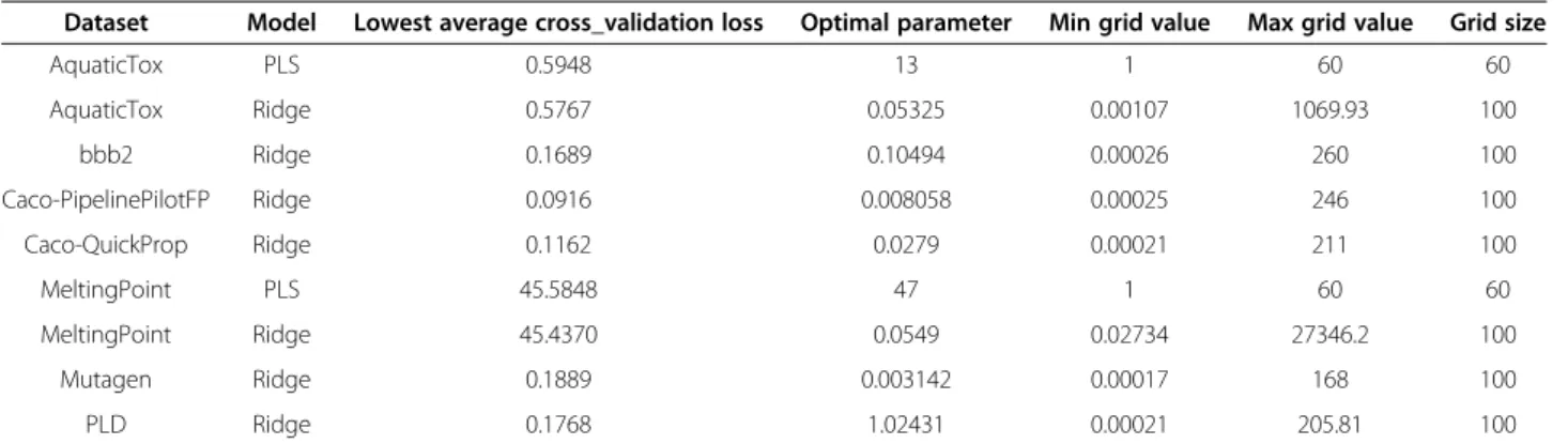
Dataset Model Lowest average cross_validation loss Optimal parameter Min grid value Max grid value Grid size
AquaticTox PLS 0.5948 13 1 60 60
AquaticTox Ridge 0.5767 0.05325 0.00107 1069.93 100
bbb2 Ridge 0.1689 0.10494 0.00026 260 100
Caco-PipelinePilotFP Ridge 0.0916 0.008058 0.00025 246 100
Caco-QuickProp Ridge 0.1162 0.0279 0.00021 211 100
MeltingPoint PLS 45.5848 47 1 60 60
MeltingPoint Ridge 45.4370 0.0549 0.02734 27346.2 100
Mutagen Ridge 0.1889 0.003142 0.00017 168 100
PLD Ridge 0.1768 1.02431 0.00021 205.81 100
Summary of selected optimal cross-validatory chosen models from nine examples.
Figure 10Cross-validation and nested cross-validation sum of squared residuals for ridge regression and PLS on AquaticTox. Boxplots of 50 cross-validation sum of squared residuals for ridge regressiona and PLS on AquaticTox and 50 nested cross-validation sum of squared residuals for ridge regressiona and PLS on AquaticTox.
the rule needs to be redefined in the repeated cross-validation context.
There are situations where the practitioner just needs to find an optimal model and the issue of its assessment is not important. In those cases, it is not necessary to perform nested cross-validation. However, in most prac-tical applications with limited sample sizes, use of pre-dictive models depends on reliable model assessment. As far as we are aware, nested cross-validation is the best non-parametric approach for model assessment when cross-validation is used for model selection. As we have mentioned before, nested cross-validation estimate is not a property of the selected model, but rather
comprises assessment of the selected model M and the protocol P used to select it. To reflect this fact, we intro-duced notation P-estimate to refer to nested cross-validation estimate of the large-sample performance of model M. As an example, consider cross-validation of linear SVM with three cost values and five folds (proto-col P1) vs. cross-validation with seventeen cost values and five folds (protocol P2), and assume the minimum error rate is achieved by the same model M (i.e., same cost) in both experiments. The corresponding nested cross-validations will, in general, yield two different P-estimates (P1-estimate and P2-estimate, respectively) of the model M performance. This is reflection of the fact that the two cross-validations scanned different regions
Figure 12Cross-validation and nested cross-validation proportion misclassified for ridge logistic regression on caco-PipelinePilotFP and caco-QuickProp.Boxplots of 50 cross-validation and 50 nested cross-validation proportion misclassified for ridge logistic regression on caco-PipelinePilotFP and caco-QuickProp.
Figure 13Cross-validation vs nested cross-validation for ridge logistic regression on bbb2.Histogram of 50 cross-validation and 50 nested cross-validation proportion misclassified for ridge logistic regression on bbb2.
Figure 14Cross-validation vs nested cross-validation for ridge logistic regression on Mutagen.Histogram of 50 cross-validation and 50 nested cross-validation proportion misclassified for ridge logistic regression on Mutagen.
of hyper-parameter space, and the two P-estimates re-flect different information incorporated into the selected best model. Thus, the P-estimates of the selected model differ, since they describe performance of different (model, protocol) pairs. We argue that this characteristic of nested cross-validation does not detract from its’ util-ity, however it is critically important to recognize it in order to properly interpret the results.
In the past, the major concern with grid search was that it was either computationally infeasible or very ex-pensive. However, with the advent of cloud computing, new concern is that its extensive use in cross-validation will generate statistical models which will overfit in prac-tice. Here we need to separate two issues:
1) How we define the optimisation problem for minimising cross-validation error estimates? 2) How we solve the optimisation problem?
As Dudoit and van der Laan [8] have shown, the first question is well defined with larger samples in V-fold cross-validation. However, Breiman et al. [25] have shown that cross-validatory chosen models are too com-plex in their examples. In the literature this issue is known as thecross-validation bias[26]. We are aware of three systematic approaches to solving this problem in the cross-validation context:
1. 1 SE rule as suggested by Breimanet al.[25] and Hastieet al.[4]
2. Corrected V-fold cross-validation as suggested by Burman [27]
3. Penalised V-fold cross-validation as suggested by Arlot [28].
Once we define an optimisation target, i.e. find parame-ters which minimise cross-validation error estimate, our aim is to find the optimal solution. Grid search is not the only systematic approach to hyper parameter optimisation. Recently Bergstra and Bengio [29] gave the case for using random search, while in the past we used Nelder and Mead [30] method. Regardless of the search method we use, the goal is to find the optimal parameter. We suggest using grid search because it is simple to implement and its parallelisation in the cloud is trivial. In our practice we prefere dense grids and the answer to question how dense is usually related to the costs.
In our findings, sparse grids do not necessarily lead to simpler models nor reduced overfitting. In all our exam-ples where we applied PLS with grid being number of components from 1 till 60 with step 1. If we had chosen a less dense grid with number of components from 5 till 60 with step 5, then on AquaticTox the cross-validatory chosen number of components would be 15 (instead of 13 as with original dense grid), while on MeltingPoint the cross-validatory chosen number of components would be 50 (instead of 47 as with original dense grid). As the consequence of using such a less dense grid, our cross-validatory chosen model on both datasets would be more complex than the original dense grid.
It is important to note that both Stone [2] and Varma and Simon [9] use leave-one-out cross-validation, while we use V-fold cross-validation. The beauty of the leave-one-out cross-validation is that it generates the same results each time it is executed, and there is no need to repeat it. So it is possible to execute only single leave-one-out cross-validation and single nested leave-one-out cross-cross-validation. However, as we have pointed out earlier, leave-one-out tends to select models with higher variances, which lead to overfitting, and for that reason we use V-fold cross-validation.
The computational cost is usually mentioned as the main drawback of nested cross-validation. In our exam-ples, we repeat 50 times 10-fold nested cross-validation which means that for nine examples we performed 500 times full model selection process, where each model selec-tion consists of 50 times repeated 10-fold cross-validaselec-tion. Various authors proposed simplifications which obviate the need for the extensive computations. Tibshirani and Tibshirani [31] propose a bias correction for the mini-mum error rate in cross-validation which does not re-quire additional computation. Bernauet al.[32] suggest another correction which would reduce the computa-tional costs associated with nested cross-validation. We propose that the computational cost of performing re-peated cross-validation and nested cross-validation in
the cloud have reached a level where the use of substi-tutes to full nested cross-validation are no longer justified.
In discovery research projects there are experimental costs associated with the training samples. At a certain point in the project, the following question is usually asked: Will the additional data improve our predictive models and, if so, by how much? If the samples are gen-erated randomly from the same population, then add-itional data will always improve the predictive model. However, the question is whether the additional costs of performing experiments will pay off in improve-ments to the model. In our opinion, here we can see the practical value of nested cross-validation. In case of Mutagen dataset, or even caco-PipelinePilotFP, where intervals of nested cross-validation errors are narrow and similar to cross-validations’, we can conclude that if we randomly remove 10% of samples, the quality of models remains almost the same. So we can say that additional increase of 10% of sample size will not sig-nificantly improve our current models.
Our results show that repetition is an essential compo-nent of reliable model assessment based on nested cross-validation. Any single nested cross-validation run cannot be used for assessing the error of an optimal model, because of its variance. We demonstrated the use of repeated nested cross-validation in order to get an interval of the estimate.
Furthermore, we demonstrated that there are datasets (for example, AquaticTox) where the interval of nested cross-validation errors is wide, and in which cases the user must assess the suitability of the model for the task in hand. We think that these situations point to the in-adequacy of the dataset itself, rather than inin-adequacy of the nested cross-validation method. In such cases the application of repeated nested cross-validation points to the need to collect additional samples/compounds and/ or alternative descriptors.
Conclusions
Selection and assessment of predictive models require re-peated cross-validation and nested cross-validation. The advent of affordable cloud computing resources makes these methods widely accessible. In our opinion, the ability to economically use large amounts of computer power over the cloud changes the perception of what is feasible and what is necessary to perform when selecting and asses-sing models.
Competing interests
DK, DEL and ST are shareholders of Cyprotex Discovery Ltd.
Authors’contributions
DK & DEL & ST initiated the study; DK & LJB & ST designed the study; DK & LJB wrote the text; DK performed data analysis. All authors read and approved the final manuscript.
Acknowledgements
We would like to thank Cyprotex Discovery Ltd for paying the costs of publishing the article. DK would like to thank dr MilošIvanovićfrom the Faculty of Science at the University of Kragujevac for his help with cloud computing. We also thank two anonymous referees who gave useful comments on an earlier draft of this article.
Author details
1Research Centre for Cheminformatics, Jasenova 7, 11030 Beograd, Serbia. 2
Laboratory for Molecular Biomedicine, Institute of Molecular Genetics and Genetic Engineering, University of Belgrade, Vojvode Stepe 444a, 11010 Beograd, Serbia.3Clinical Persona Inc, 932 Mouton Circle, East Palo Alto, CA 94303, USA.4Molplex Pharmaceuticals, Alderly Park, Macclesfield SK10 4TF,
UK.5Cyprotex Discovery Ltd, 15 Beech Lane, Macclesfield SK10 2DR, UK.
Received: 6 January 2014 Accepted: 25 March 2014 Published: 29 March 2014
References
1. Allen DM:The relationship between variable selection and data agumentation and a method for prediction.Technometrics1974, 16(1):125–127.
2. Stone M:Cross-validatory choice and assessment of statistical predictions.J Roy Stat Soc B Met1974,36, No. 2:111–147.
3. Geisser S:The predictive sample reuse method with applications.J Am Stat Assoc1975,70(350):320–328.
4. Hastie T, Tibshirani R, Friedman J:The elements of statistical learning.New York: Springer; 2009.
5. Breiman L, Spector P:Submodel selection and evaluation in regression. The x-random case.Int Stat Rev1992,60(3):291–319.
6. Kohavi R:A study of cross-validation and bootstrap for accuracy estimation and model selection.InIJCAI.; 1995:1137–1145.
7. Chang CC, Lin CJ:LIBSVM: a library for support vector machines.ACM Transactions on Intelligent Systems and Technology (TIST)2011,2(3):27. 8. Dudoit S, van der Laan MJ:Asymptotics of cross-validated risk estimation
in estimator selection and performance assessment.Stat Meth2005, 2(2):131–154.
9. Varma S, Simon R:Bias in error estimation when using cross-validation for model selection.BMC Bioinformatics2006,7(1):91.
10. Ambroise C, McLachlan GJ:Selection bias in gene extraction on the basis of microarray gene-expression data.Proc Natl Acad Sci2002,
99(10):6562–6566.
11. Zhu X, Ambroise C, McLachlan GJ:Selection bias in working with the top genes in supervised classification of tissue samples.Stat Meth2006, 3(1):29–41.
12. QSARdata.http://cran.r-project.org/web/packages/QSARdata. 13. He L, Jurs PC:Assessing the reliability of a QSAR model’s predictions.
J Mol Graph Model2005,23(6):503–523.
14. Burns J, Weaver DF:A mathematical model for prediction of drug molecule diffusion across the blood–brain barrier.Can J Neurol Sci2004, 31(4):520–527.
15. Pham-The H, González-Álvarez I, Bermejo M, Garrigues T, Le-Thi-Thu H, Cabrera-Pérez MÁ:The use of rule-based and QSPR approaches in ADME profiling: a case study on caco-2 permeability.Molecular Informatics2013, 32(5–6):459–479.
16. Karthikeyan M, Glen RC, Bender C:General melting point prediction based on a diverse compound data set and artificial neural networks.J Chem Inf Model2005,45(3):581–590.
17. Kazius J, McGuire R, Bursi R:Derivation and validation of toxicophores for mutagenicity prediction.J Med Chem2005,48(1):312–320.
18. Goracci L, Ceccarelli M, Bonelli D, Cruciani G:Modeling phospholipidosis induction: reliability and warnings.J Chem Inf Model2013,53(6):1436–1446. 19. e1071.http://cran.r-project.org/web/packages/e1071.
20. Hoerl AE, Kennard RW:Ridge regression iterative estimation of the biasing parameter.Commun Stat1976,5(1):77–88.
21. Friedman J, Hastie T, Tibshirani R:Regularization paths for generalized linear models via coordinate descent.J Stat Software2010,33(1):1. 22. glmnet.http://cran.r-project.org/web/packages/glmnet.
24. pls.http://cran.r-project.org/web/packages/pls.
25. Breiman L, Friedman JH, Olshen RA, Stone CJ:Classification and regression trees.Monterey, CA: Wadsworth & Brooks; 1984.
26. Arlot S, Celisse A:A survey of cross-validation procedures for model selection.
Stat Surv2010,4:40–79.
27. Burman P:A comparative study of ordinary cross-validation, v-fold cross-validation and the repeated learning-testing methods.Biometrika
1989,76(3):503–514.
28. Arlot S:V-fold cross-validation improved: V-fold penalization.arXiv preprint arXiv:0802.05662008:.
29. Bergstra J, Bengio Y:Random search for hyper-parameter optimization.
J Mach Learn Res2012,13:281–305.
30. Nelder JA, Mead R:A simplex method for function minimization.Comput J1965,7(4):308–313.
31. Tibshirani RJ, Tibshirani R:A bias correction for the minimum error rate in cross-validation.Ann Appl Stat2009,3(1):822–829.
32. Bernau C, Augustin T, Boulesteix AL:Correcting the optimal resampling‐based error rate by estimating the error rate of wrapper algorithms.Biometrics
2013,69(3):693–702.
doi:10.1186/1758-2946-6-10
Cite this article as:Krstajicet al.:Cross-validation pitfalls when selecting and assessing regression and classification models.Journal of Cheminformatics20146:10.
Open access provides opportunities to our colleagues in other parts of the globe, by allowing
anyone to view the content free of charge.
Publish with
Chemistry
Central and every
scientist can read your work free of charge
W. Jeffery Hurst, The Hershey Company.
available free of charge to the entire scientific community peer reviewed and published immediately upon acceptance cited in PubMed and archived on PubMed Central yours you keep the copyright
Submit your manuscript here: