Vol 10, No 3 (2018)

(1)

International Journal of Communication Networks and Information Security (IJCNIS) Vol. 10, No. 3, December 2018

BotCap: Machine Learning Approach for Botnet

Detection Based on Statistical Features

Mohammed S. Gadelrab

1

_{, Muhammad ElSheikh}

1, 2

_{, Mahmoud A. Ghoneim}

1, 3

_{and Mohsen Rashwan}

4

1_{IT Metrology Lab, National Institute for Standards, Egypt}

2 _{Institute for Information Systems Engineering (CIISE), Concordia University, Canada}

3 _{Computer Science Department, School of Engineering and Applied Science, George Washington University, USA} 4 _{Communication Engineering Department, Faculty of Engineering, Cairo University, Egypt}

Abstract: In this paper, we describe a detailed approach to

develop a botnet detection system using machine learning (ML) techniques. Detecting botnet member hosts, or identifying botnet traffic has been the main subject of many research efforts. This research aims to overcome two serious limitations of current botnet detection systems: First, the need for Deep Packet Inspection-DPI and the need to collect traffic from several infected hosts. To achieve that, we have analyzed several botware samples of known botnets. Based on this analysis, we have identified a set of statistical features that may help to distinguish between benign and botnet malicious traffic. Then, we have carried several machine learning experiments in order to test the suitability of ML techniques and also to pick a minimal subset of the identified features that provide best detection. We have implemented our approach in a tool called BotCap whose test results proved its ability to detect individually infected hosts in a local network.

Keywords: Security, Botnet, Botware, Malware Analysis,

Malware Detection, Machine Learning.

1. Introduction

The Internet reflects both the good and the bad sides of the physical world. With the emergence of the Internet, new kinds of crime –namely cybercrimes– have been flourishing and spreading. The new criminals have various goals and tools. Malware “malicious software” is considered as the main tool in the hands of cyber-criminals.

Today, new generations of malware are becoming multi-faceted and more modular. Botnets are one of these outcomes. Botnet – robot network – is a network of Internet-connected, compromised hosts (also known as bots, bot-clients, or zombies). Bots are remotely controlled by an attacker called botmaster via a Command-and-Control (C&C) channel. C&C channels often take place over existing network protocols including Internet Chat Rely (IRC), Hypertext Transfer Protocol (HTTP), or other Peer-To-Peer protocols (P2P). Botnets can be categorized, based on C&C system, into centralized and decentralized botnets. The centralized botnet has a form of traditional client-server network model. A bot acts as a client-side and connects to a central C&C server. In decentralized botnets, any bot can act as a C&C sever for some other bots instead of a central C&C server. Bots serve as a proxy infrastructure and a launch base for a wide variety of cyber attacks such as sending SPAM emails, launching Distributed Denial-of-Service (DDoS), performing identity theft, click frauds, etc.

In our research on botnets, we tackled the problem in different ways: analysis, modelling, and detection. Firstly, we have deeply analyzed various botware samples using several analysis approaches (static, dynamic and network). As a result, we managed to model bots life-cycle in a generic

model that improves our ability to both understand and respond to botnet threats. Moreover, motivated by the lack of public representative botnet dataset, we have created our BoTGen platform. It is implemented from off-the-shelf open source software to provide researchers with a flexible, reliable and fully automated platform. This allows not only to produce datasets but also to experiment with various and complete botnet scenarios in a controlled environment [14]. The work described in this paper employs Machine Learning techniques (Decision Tree and Support Vector Machine) to build a botnet detection system: BoTCap. The goal is to detect bots independently from their C&C structure and protocol. The results showed that our tool can detect bot infections with high detection rates up to 80% and 95 % for HTTP and IRC based botnet respectively and very small false positive rates of nearly 0.05% and 0.025% respectively. Because of the shortcomings that we identified in several of the previous work (Section 2), we had to design and implement another approach to alleviate the following limitations:

1. Detecting only well-known botnets based on signatures extracted from binary codes of the malwares (host-based) or extracted from network payloads of malicious activities (network-based). These approaches often fail in detecting bots that are infected by new botware or botware that uses obfuscation techniques (host-based) and encrypted traffic (network-based).

2. Being computationally expensive and violates the privacy. For example, in case of network-based approaches that perform deep packet inspection (DPI) for each packet. 3. Detecting some botnet types and ignoring others. For example, detect http-based only or detect IRC-based only. 4. Detecting only bots that participate in massive malicious activities such as DDoS, spamming and click fraud while it cannot detect stealthy or dormant attacks. Such bots include usually perform few activities over time to keep undetectable. These could be dangerous because they are often employed in spying and stealing sensitive data (e.g., credit cards or login credentials).

5. Inability to detect individually infected hosts that belong to botnets. In other words: it does not require data correlation from several bots to be able to detect botnets.

(2)

2. Related Work

Several research work focused on machine-learning-based approaches for botnet detection. Livadas et al. [35] proposed one of the first attempts to utilize ML algorithms to detect IRC-based botnets. The authors evaluate several supervised ML algorithms to classify IRC-based botnet traffic using a set of network statistical features such as bits-per-second, packets-per-second, flow duration, etc. The traffic classification is performed in two sequential stages. The first stage classifies the traffic into chat-like (IRC) and non chat-chat-like classes. The second stage separates the chat-like class into malicious and non-malicious sub-classes. The authors proposed a novel botnet detector based on network statistical features only.

BotMiner [21] detection system is independent of C&C protocol and botnet structure. It can be considered as the extended and complementary work of BotSniffer [22]. BotMiner performs the horizontal behavioral correlation among the local hosts with interest in differentiation between the concept of communication activities “Who is talking to whom” and malicious activities “Who is doing what”. BotMiner consists of three main parts. The first part is responsible for the communication activities (C-plane). It monitors the traffic flows between internal hosts and the externals. Each group of flows (C-flows) that share the same 4-tuple (SrcIP, DstIP, DstPort, and Protocol) are represented by a vector of 52 elements extracted from four main network statistical features named: the number of flows per hour (fph), the number of packets per flow (ppf), the average number of bytes per packets (bpp), and the average number of bytes per second (bps). Then, it applies two-steps X-means clustering algorithm to aggregate hosts that share the same communication activities. The second part of BotMiner is responsible for malicious activities (A-plane). By using the malicious activities detector from BotSniffer, it detects the hosts that are involved in each of scan activity, SPAM activity, and binary download activity. After that, BotMiner applies two-step clustering algorithm to aggregate the hosts involved in the same malicious activities. The final part of BotMiner is a cross-plane correlation function. It combines the results from C-plane and A-plane to calculate a score for each host. Host scores depend on weighted clusters that indicate host membership. A host is declared bot if its score is larger than a threshold. The major weakness of BotMiner is the biased score function; if a host is not involved in any malicious activities (or undetectable), it will be classified as a benign whatever its communication activities. Besides that, it requires multiple infections by the same botware in the local network in order to be detectable.

Traffic Aggregation for Malware Detection (TAMD) [23] aims to detect infected hosts in local networks. TAMD uses the collected traffic at the edge of the local network to aggregate local hosts that share similar three characteristics: destination, payload, OS platform. Each characteristic have its aggregation function which utilizes ML algorithms. The results of the three aggregation functions are then combined in a rule-based system to detect bots. TAMD aggregation is similar to the horizontal correlation in BotSniffer and BotMiner while the behavioral characteristics are different.

Tegeler et al. [24] utilize ML algorithms to build network-based signatures that can differentiates between botnet families. The proposed system, named BotFinder, is used to detect HTTP-based botnet using only five network statistical features. BotFinder is based on the observation that the traffic between C&C and bots in pulling mode botnet (e.g., HTTP-based botnets

follow that mode) often has regularity in contents and regularity in time. It analyzes network traces to calculate five features: (1) The average time interval between two sequential flows in the trace, (2) The average duration of flows, (3, 4) The average number of bytes per flow sent from source to destination and from destination to source respectively, and (5) The most significant frequency of Fast Fourier Transform (FFT) that uses start time of flows as a time signal. BotFinder has low false positive similar to signature-based systems however, its accuracy is lower than traditional signature-based. It could be biased to botnet configuration rather than botnet family itself.

Zhang et al. [25] proposed a new packet sampling and spatial-temporal flow correlation approach to identify suspicious hosts that are most likely bots. It applies packet sampling techniques to adapt BotMiner and BotSniffer to work in a high speed network. All the aforementioned approaches, except BotMiner, focus on detecting centralized botnets. Approaches in [26, 27, 28, 29, 30] aim to detect P2P botnet.

Yen et al. [26] proposed an algorithm to separate hosts that run legitimate P2P file sharing applications from P2P bots. The proposed system uses features related to traffic volume, persistence of network connections, and differences between human-driven and machine-driven traffic. The features are extracted from traffic summaries without DPI. However, the proposed system does not take into account other legitimate P2P applications such as Skype rather than P2P file sharing applications. It also misclassified hosts that are running P2P botware and P2P file sharing together.

Zhang et al. in [29, 30] proposed a detection system capable of detecting stealthy P2P botnets without dependency on any malicious activities. First, the system separates the hosts that are engaged in P2P communications. Then, it derives statistical fingerprints of the P2P communications corresponding to different P2P applications. Finally, the system distinguishes between P2P benign hosts and P2P bots based on two observations: (1) P2P bots expose persistent connection and the active time of P2P connection is comparable to the active time of the host, (2) bots belonging to the same P2P botnet have a high overlap of their sets of contacted IPs (simple horizontal correlation). This technique needs two or more hosts infected by the same botnet to observe the overlap between their sets of contacted IPs (i.,e., can not catch single infection). Moreover, it needs to have fingerprints for all legitimate P2P application which is infeasible.

J. Wang et al. [1] proposed a two-stage approach for botnet detection. During the first stage, it statistically analyzes network flow to detect anomalies that could be a sign of botnet. In the 2nd stage, it analyzes network interactions between hosts to detect highly co-related hosts using social correlation graphs. Although this approach is protocol agnostic, it relies on the presence of group activities to be able to detect botnets.

(3)

Similar to our approach on feature selection, Nur Hidayah et al. [3] have analyzed the influence of feature selection on the detection of only HTTP-based botnets.

3. Approach and Basic Evaluation Metrics

The idea behind this approach stems from the basic observation that common patterns in botnet traffic often have some similarity in both traffic contents and the regularity in time. Theoretically, botnet detection can be performed based on the observation of several types of botnet interactions between botnet elements: botmaster, C&C, individual bots and the surrounding environment. Deciding which interactions or activities to observe depends on several factors such as botnet architecture, network protocols as well as the ease of capturing or identifying some botnet interaction.

Generally, botnet communication can be divided into three segments: Botmaster<=>C&C segment (Seg1), C&C<=>Bot segment (Seg2), and Bot<=>Bot or Bot<=>Other segment (Seg3) as shown in Figure 1. C&C point may be single C&C server in case of centralized botnet or it could be several distributed points, where any bot can act as a C&C server for its peer bots like in P2P-based botnet. Communications on Seg1 are difficult to observe due to its sparse occurrence. Bots are more frequently involved in interactions that occur on Seg2 and Seg3. C&C and bots connects together either to receive commands or to update status (Seg2). Bots also interacts with each other in P2P botnets or with any other node outside the botnet to carry out malicious activities on Seg3. Thus, in case of centralized botnets (e.g., IRC or HTTP), a detection method based on C&C activities in Seg1&2 could be more appropriate because it may help in discovering connected bots as well as their botmaster. In case of P2P botnets, the concept of dedicated centralized C&C server does not exist. Therefore, communications in Seg3 are more appropriate where interactions and activities between individual bots take place.

Figure 1. Botnet Communication Segmentation The system that we describe hereafter uses network-flow information. This choice eliminates the need to inspect packet payloads, which has several advantages. First, no processing overhead of deep packet inspection, which improves system performance. Second, no inspecting packet contents means implicitly no privacy violation. Finally, the system becomes more resilient to encrypted traffic.

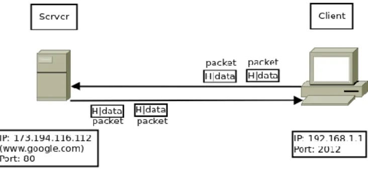
Besides that, our approach concentrates on botnet traffic that is related to maintenance/control messages that may be exchanged on segment Seg2 in case of centralized botnets or Seg3, in case of peer-2-peer. This enables the detection of dormant bots that do not send significant quantity of traffic, for example to spam or to carry out DDoS attacks. More precisely, we focus on TCP/IP network flow, which is a set of packets between any communicating pair that have 5 features in common: ScrIP, ScrPort, DstIP, DstPort and

Protocol. Using this 5-tuple features as a flow identifier makes each flow unique in the network segment. The flow can be bidirectional like TCP flows or unidirectional like UDP flows. Figure 2 illustrates a typical example of client-server flow where the 5-tuples are: ScrIP=192.168.1.1, SrcPort=2012, DstIP=173.194.116.112, DstPort=80 and Protocol = TCP, HTTP application uses TCP as transport layer protocol. TCP/IP Trace or traffic trace for simplicity, is an aggregation of TCP/IP flows between any client-server pair during a certain period of time. The flows are aggregated based on their values of 3-tuple (SrcIP, DstIP, and DstPort). The approach consists simply of analyzing a set of statistical features of traffic traces to identify signs of bot communication in terms of similarity and regularity or repetitiveness. To implement this approach in BotCap, we have to go through two essential stages:

1. Feature Selection: in this part, we analyzed a lot of statistical features of traffic traces to pick up and define an initial set of distinctive features that seems to be helpful in botnet detection.

2. Building ML detection model: in this part, we deal with ML model creation process. We employ J48, which is a variation of C4.5 algorithm [5] and different SVM kernels [6], [7] to identify a feature set that gives good detection results for the same ML algorithm. Then, we compare results of different algorithms to select the one producing the best results.

This process requires a dataset that contains malicious and benign traffic. It will be used for training and testing ML algorithms, as well as feature set optimization and reduction. For this purpose, we have created a diversified dataset as described in [14]. In the following section we present the metrics used in evaluating and comparing detection results from various ML models/algoritms and feature-sets.

Figure 2. TCP/IP network flow

Our evaluation criteria is based on three basic metrics: Precision, Recall and F1-Measure. These metrics are derived to assess the quality of detection results. The following concepts represent some definitions:

• TP: True Positive = the number of items correctly classified as belonging to the positive (Malicious/Botnet) class.

• FN: False Negative = the number of items that is actually belonging to the (Malicious/Botnet) positive class but misclassified as belonging to the negative (Benign) class. • TN: True Negative = the number of items correctly

classified as belonging to the negative (Benign) class. • FP: False Positive = the number of items that is actually

(4)

• Confusion matrix:

Actual class Positive Negative Classified

class

Positive TP FP

Negative FN TN

• Precision: From all items classified as a positive class, which portion is actually belonging to a positive class?

Eq. (1)

Recall: also known as True Positive Rate (TPR) or sensitivity. From all items that actually belong to positive class, which portion are correctly classified as positive class?

Eq. (2)

F1-measure: a combined measure that assesses the Precision and Recall trade-offs. It is equivalent to the weighted harmonic mean of Precision and Recall

Eq. (3)

4. Feature Selection

Botnet interactions can be observed from different view points. For example, botnet manifestations may appear at network level or system level where we can collect data about their activities by recording network traffic or system calls, respectively. It is worth to note that while both views complement each other, the network view provides a more comprehensive view of botnet activities. Due to the multidimensional nature of botnets, we can obtain hundreds of features, which complicates feature selection. To filter this huge number of features and to obtain only botnet-relevant features, we defined the following criteria to be satisfied in the selected features:

(a) Be independent from packet payload contents. (b) Be independent from botnet or botware type. (c) Can capture regularity in botnet traffic contents.

(d) Can capture regularity or repetition in time (periodicity). In order to provide network-wide botnet detection, we decided to focus on network-based features. Besides that, statistic-based features can be easily obtained or calculated from packet headers or by counting transmitted/received packets independently from both botnet/botware types and packet contents. It can also capture similarities and regularities in botnet traffic. Moore et al. [8] have identified a lot of statistical features extracted from packet header fields to help in network classification per flow. Riyad et al [9] present another set of statistical features to classify encrypted VOIP traffic. We have analyzed these features to eliminate irrelevant features for botnet detection. To explain that, we can divide statistical features extracted from network traffic into three categories based on the characteristics of:

(a) the network itself (network configuration) such as number of packets per second, number of bits per second, packet inter arrival time.

(b) general botnet behavior: for example, flow rate, flow duration, time interval between successor flows.

(c) particular botnet family: such as number of packets per flow, packet size, window size, number of packets coming from server/client.

In our case, candidate features should characterize general botnet features and with less extent botnet family features; because our goal is to detect bots not to identify botnet families. Features that are network-dependent are completely excluded to make our approach suitable for any type of network regardless of its speed, bandwidth, topology, etc. Regarding the regularity in contents or time, features of individual packets cannot capture such properties and hence are excluded. The regularity and repetition can be better observed in aggregate traffic not individual packets. The question that may arise now is about the aggregation level. For example, should the features be calculated for traces or flows? The desired set of features can be calculated per flow or from aggregated set of flows (i.e., per trace). In general, an individual flow provides a limited view about what happens inside botnets or describes action/response on the C&C-bot segment at certain instance of time. On the other hand, the mean of observed features can reflect the regularity in content and connections over time between C&C and each bots. For this reason, we calculate features per trace during certain time epoch.

4.1. Content-Regularity Features

Regularity in content arises from repeated command-response patterns. Bots are often pre-programmed with predefined hard-coded responses. They respond to the same command in a similar manner. From start-up to shutdown time, bot can be in two modes, active mode and idle mode. The bot becomes in active mode when it receives a command from C&C. After the bot executes a command, it returns back to idle mode. In idle mode, the bot only connects to its C&C to check for new commands and update its status. In particular, regularity in traffic contents comes from:

• In idle mode, fixed format to check new commands and fixed format to update its status.

• In active mode, same commands has similar reactions with some variation in the response traffic.

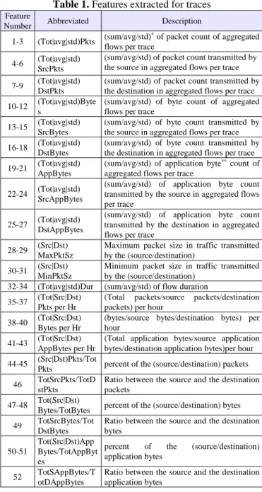
Content regularity can be observed through statistical features such as average number of packets per trace for both source and destination. Table 1 summarizes candidate features that initially satisfies our selection criteria.

4.2. Periodicity Features

Concerning time regularity (periodicity), for example HTTP-based botnets have an explicit period where bots follow the pulling mode. The botmaster sends new commands to C&C server, then each bot periodically checks the C&C server for new commands. On the other hand, IRC-based botnets demonstrate different kind of periodicity where bots does not follow pulling mode and follow instead the pushing mode. When the botmaster sends new commands to C&C server, the C&C server instantly re-sends these commands to the bots. The periodicity comes from the C&C server itself where IRC protocol has a test mechanism to detect the presence of active clients by sending PING or REQUEST messages at regular intervals.

Dealing with periodicity needs each network trace represented as a time-periodic signal. There are several time-periodic signals that can characterize botnet traces, for example:

(5)

2. Throughput of down-link (bytes per second transfer from C&C to bots)

3. Throughput of up-link (bytes per second transfer from bots to C&C)

Table 1. Features extracted for traces Feature

Number Abbreviated Description

1-3 (Tot|avg|std)Pkts (sum/avg/std)_{flows per trace}* of packet count of aggregated

4-6 (Tot|avg|std) _SrcPkts (sum/avg/std) of packet count transmitted by _{the source in aggregated flows per trace}

7-9 (Tot|avg|std) DstPkts

(sum/avg/std) of packet count transmitted by the destination in aggregated flows per trace

10-12 (Tot|avg|std)Byte_s (sum/avg/std) of byte count of aggregated _{flows per trace}

13-15 (Tot|avg|std) _SrcBytes (sum/avg/std) of byte count transmitted by _{the source in aggregated flows per trace}

16-18 (Tot|avg|std) _DstBytes (sum/avg/std) of byte count transmitted by _{the destination in aggregated flows per trace}

19-21 (Tot|avg|std) _AppBytes (sum/avg/std) of application byte_{aggregated flows per trace} ** count of

22-24 (Tot|avg|std) _SrcAppBytes

(sum/avg/std) of application byte count transmitted by the source in aggregated flows per trace

25-27 (Tot|avg|std) _DstAppBytes

(sum/avg/std) of application byte count transmitted by the destination in aggregated flows per trace

28-29 (Src|Dst) _MaxPktSz Maximum packet size in traffic transmitted _{by the (source/destination)}

30-31 (Src|Dst) _MinPktSz Minimum packet size in traffic transmitted _{by the (source/destination)}

32-34 (Tot|avg|std)Dur (sum/avg/std) of flow duration

35-37 (Tot|Src|Dst) Pkts per Hr

(Total packets/source packets/destination packets) per hour

38-40 (Tot|Src|Dst) _{Bytes per Hr} (bytes/source bytes/destination bytes) per _hour

41-43 (Tot|Src|Dst) _{AppBytes per Hr} (Total application bytes/source application _{bytes/destination application bytes)per hour}

44-45 (Src|Dst)Pkts/Tot_Pkts percent of the (source/destination) packets

46 TotSrcPkts/TotD_stPkts Ratio between the source and the destination _packets

47-48 Tot(Src|Dst) _{Bytes/TotBytes} percent of the (source/destination) bytes

49 TotSrcBytes/Tot DstBytes

Ratio between the source and the destination bytes

50-51

Tot(Src|Dst)App Bytes/TotAppByt es

percent of the (source/destination) application bytes

52 TotSAppBytes/T_otDAppBytes Ratio between the source and the destination _{application bytes}

*_{sum=summation, avg=average, std=standard deviation} **_{Application Bytes mean payload of packets without any header}

Periodicity features will be calculated for all traces; both malicious and benign. Because bots reside in client side of sever/client pairs, we can calculate the throughput over seconds of up-link connections (in our case a = 5 second) for each bot, as shown in Figure 3 (a), the throughput is represented as semi-periodic impulse train. As a time signal, it corresponds to a finite time impulse and noisy signal. There are many techniques to check whether the time signal is periodic or not. The most used method is to analyze the signal in frequency domain and obtain the peaks to determine the frequency. The power estimation is one of frequency domain signals that characterizes the time signal. Welch's method is an approach for spectral density estimation that provides a method for estimating the power of time signal at

different frequencies [11]. the improvement of Welch's method over the standard periodogram spectrum estimation method is that it reduces noise in the estimated power spectra. Due to the noise caused by imperfect and finite data, the noise reduction from Welch's method is often desired.

Figure 3(a). Up-link Throughput in time domain, (b). Up-link Throughput in frequency domain

We developed a simple algorithm (Code.1) using Welch's method implemented in Numpy & SciPy package [12], [13] to check the periodicity of the up-link traffic throughput per trace. If periodic, it calculates the frequency. The algorithm has three main steps. The first step is to transfer the up-link throughput from time domain to frequency domain using Welch's method. The next step is to check if the signal is periodic or not by passing three check points as follows: 1- if trace duration is less than MIN_DURATION (in our case = 60 minutes), this trace will be assigned as not periodic (is_periodic = -2) because Welch's method is based on window FFT calculation which depends on the number of samples and the sampling rate of the signal.

2- Count the number of peaks in the power signal over threshold, see Figure 3(b). If the number of peaks is less than MIN_NUM_of_PEAKS (in our case = 3, arbitrarily selected), this trace will be assigned as not periodic (is_periodic = -1). The throughput in time domain is a noisy impulse train and it will be so in frequency domain. Therefore, the more number of peaks increase the probability of periodicity.

3- Calculate the average (freq) and the standard deviation (stdfreq) of frequency difference of the first three peaks, see Figure 3(b). If stdfreq is larger than gamma percent from freq (in our case gamma = 10%) then this trace will be assigned as not periodic (is_periodic = 0) otherwise this trace will be periodic (is_periodic = 1).

(6)

Code 1. Periodicity Detection Algorithm. Table 2. Periodicity features for traces

Feature

Number Name Description

53 is_periodic

{1,0,-1,-2}

1: uplink throughput is periodic

0: not periodic due to stdfreq > 10% of freq -1: not periodic duo to # of peaks less than 3 -2: not periodic due to trace duration < 60 minutes

54 freq average of frequency difference of the first _{three peaks of Welch's spectral}

55 stdfreq standard deviation of frequency difference of _{the first three peaks of Welch's spectral}

5. Detection Model Design and Implementation

In this section, we describe the process that we followed to create and test the suggested botnet detection mechanism using machine learning algorithms, namely J48 and different SVM kernels. As shown in Figure 4, this process includes: (1) creating datasets (malicious dataset and benign dataset) which is used in training and testing the model, (2) selecting candidate feature subsets from the primary set of features that were identified in the previous section, (3) tuning the parameters of the suggested ML algorithms, (4) creating a detection model using selected feature subsets from step 2 and using the parameters of ML obtained from step 3, (5) selecting the model that gives the highest detection results, and (6) testing that model using another dataset, that neither used in training nor in tuning phases.

The output of this process is three detection models: HTTP-only to detect HTTP-based botnets, HTTP-only to detect IRC-based botnets, and TOTAL to detect both IRC and HTTP-based botnets. The remaining of this section describes these six steps in more details.

Figure 4. Creating and testing botnet detection mechanism 5.1. Dataset Creation

The dataset consists of two components: malicious and benign. To construct the training and tuning dataset, we use six botware families: (Aryan [15], [16], Ngr [17]–[19], Rxbot [20]) as IRC-based and (Blackenrgy [31], [32], Zeus [33]–[34], Vertexnet [36]–[38]) as HTTP-based to create the malicious part of the dataset. Our decision to include these botwares was based on a detailed analysis of several botware samples where we take into account the diversity of the dataset. More details about our analysis results can be found in [14]

By using BoTGen, we run 6 botware variations from each family for 6 hours separately on 10 virtual machines (VMs). Variations differ from each other in botnet and network configuration such as (PING/PONG IRC rate, HTTP request rate, start-up/shutdown of VMs) and the executed scenario (number of commands, order of commands, etc.).

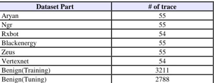
Regarding the benign dataset, we have analyzed a lot of benign datasets that were created by academic and industrial organizations. Among the analyzed datasets, we selected the UNIBS-2009 dataset [39] as it fits our goal. This dataset was created by the telecommunication network group of the university Brescia in Italy. It was captured from the edge router of the university campus network that serves (20) workstations running the GT client daemon -the Ground Truth (GT) system [39]. The traffic includes wide range of protocols such as Web (HTTP and HTTPS), Mail (POP3, SMTP, IMAP4), Skype, traffic generated by P2P applications, and other protocols (FTP, SSH, and MSN). To construct the benign part of the training dataset, we include 6-hours traffic from UNIBS-2009 dataset. Table 3 summarizes the number of traces included in the entire training dataset.

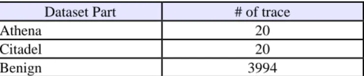
As shown in Table 4 for testing dataset, it was similarly created using botware samples that were unseen previously in the training dataset. Two botware samples: Athena [40] as IRC-based and Citadel [41], [42] as HTTP-IRC-based to create the malicious part of the testing dataset. Two variations from each botware run for 6 hours on 10 VMs. The benign part was created in the same way using another 6-hours from UNIBS dataset.

Table 3. Summary of training dataset contents.

Dataset Part # of trace

Aryan 55

Ngr 55

Rxbot 54

Blackenergy 55

Zeus 55

Vertexnet 54

Benign(Training) 3211

Benign(Tuning) 2788

Input: throughput_trace, ratio

Output: is_periodic ∈ {−2,−1,0,1}, freq, stdfreq

begin

getTraceDuration(throughput_trace)

if trace_duration < Min_DURATION then Set is_periodic = -2, freq = 0, stdfreq = 0 else

/* Calculate Welch power spectral density of throughput_trace */

/* P: Power spectral density component corresponds to (f) frequency component */

f, P = Welch(throughput_trace) global_peak = max(P)

threshold = ratio *( 0.5 * global_peak) + (1- ratio)* average(P)

peaks, peaks_val = find_peaks(P, threshold)

if number_of_peaks < MIN_NUM_OF_PEAKS then Set is_periodic = -1, freq =0 stdfreq = 0 else

freq = average(f(peaks)) stdfreq = std(f(peaks))

if stdfreq > gamma * freq then set is_periodic = 0 else

set is_periodic = 1 end

(7)

Table 4. Summary of testing dataset contents

Dataset Part # of trace

Athena 20

Citadel 20

Benign 3994

5.2. Feature-Set Reduction and Optimization

As explained in Section 4, the primary feature set consists of 55 features that may have some redundant or interdependent features. To enhance the performance, we had to reduce the number of features and select candidate subsets of the primary set. To achieve that, we have applied two selection methods: ML algorithm for attribute selection as implemented in Weka [4] and manual selection based on J48-ML experimental results. Consequently, we obtained 9 feature subsets as shown in Table 5. The features are represented as an absolute value (NotNormalized) or normalized value (Normalized). The normalization process aims to scale feature values in the range [0, 1]. Weka applies “BestFirst” as a search algorithm and “CfsSubsetEval” (Correlation-based Feature Subset Selection) as an evaluation method.

Table 5. Summary of candidate feature subsets.

ID Feature set _features# of Note

1 {Primary} 55

2 {stdDur, TotBytes/hour, TotSrcPkts/TotPkts, is_periodic, Frequency, avgTotPkts} 6

Using “select attributes” machine learning algorithm on IRC-only dataset 3 {avgSrcPkts, SrcMinPktSz, is_periodic, Frequency, TotSrcBytes, SrcMaxPktSz} 6

Using “select attributes” machine learning algorithm on HTTP-only dataset

4 {3} – _{{SrcMaxPktSz}} 5 Manual selection by removing _{SrcMaxPktSz from set-3}

5 {4} – {Frequency} 4 Manual selection by removing Frequency from set-4

6 {2} – {Frequency} 5 Manual selection by removing Frequency from set-2

7 {6}–

{TotSrcPkts/TotPkts} 4

Manual selection by removing “TotSrcPkts/TotPkts“ from set-6

8 {6} – {avgTotPkts} 4 Manual selection by removing avgTotPkts from set-6

9 {SrcMinPktSz, is_periodic, Frequency, TotDstPkts} 4

Using “select attributes” machine learning algorithm on combined (HTTP+IRC) datasets

5.3. Parameter Selection

In general, ML can be considered as an optimization problem [43]. There are many factors that may affect the performance of ML algorithms such as features, quality and quantity of dataset used in training. Moreover, the ML algorithm itself may have parameters that control its function (hyper-parameter). To optimize ML learning algorithms, their parameters should be set appropriately. In the following, we explain various parameters of the two ML algorithms that we use (i.e., J.48 and SVM). Then we present parameter values that produce best results during our experiments on each feature subset according to F1-measure as a performance indicator. There are several methods for hyper-parameter optimization problem such as [43], [44], [45]. Grid-search is a simple mechanism that scans all or subset of values in

the parameter space of a ML algorithm to obtain the optimized value. Grid-search is performed in two sequential steps: coarse-grained to enclose the optimized value in a small region on the parameter space, then fine-grained where the search is preformed in this small region to determine the optimized value. The grid-search algorithm must be guided by some performance metric, typically measured by cross-validation (CV) on the training set. Normally, botnet datasets contain a number of positive instances “malicious instances” much less than the number of negative instances “benign instances”. In other words, botnet datasets are some kind of imbalanced dataset. Therefore, F1-measure could be a good performance metric to assess the detection model and to guide grid search algorithm [46]. Our version of grid-search algorithm performs a 5-fold cross-validation (CV) on the training dataset and selects the hyper-parameter values that give the highest F1-measure. In the following, we present the hyper-parameters for both J48 and different kernels of SVM and the corresponding optimal values for each candidate feature subset based on our training dataset. The optimization has been carried out on both the Normalized and the NotNormalized values of the features.

• J48 has two parameters:

1. confidenceFactor – C: The confidence factor is used for pruning (smaller values incur more pruning). It reduces the size of the tree (or the number of nodes) to avoid unnecessary complexity and to avoid over-fitting of the dataset when classifying new data. C-parameter can be assigned values in the range of [0, 1], therefore we test C in the range from 0.05 to 1.0 by an increment step of 0.05. 2. minNumObj – M: The minimum number of instances per leaf, M ≥ 1. We test M in the range from 1.0 to 20 by an increment step of 1.0.

For each feature subset, Table 6 presents C and M values that produce best results for 18 candidate feature subsets (nine NotNormalized + nine Normalized).

Table 6. J48 Hyper-parameter values for HTTP-only, IRC-only, and TOTAL

Feature set ID

HTTP-only IRC-only TOTAL

NotNormaliz ed Normalized NotNormali zed Normalized NotNormali zed Normalized

C M C M C M C M C M C M

1 0.55 9 0.45 2 0.55 5 0.55 5 0.35 2 0.35 1

2 0.55 3 0.05 1 0.4 2 0.1 1 0.05 1 0.05 1

3 0.55 8 0.05 1 0.55 1 0.55 1 0.1 1 0.25 1

4 0.05 8 0.05 1 0.55 1 0.55 1 0.05 1 0.05 1

5 0.05 8 0.2 1 0.05 2 0.55 2 0.5 1 0.5 1

6 0.55 3 0.1 1 0.05 1 0.5 1 0.05 1 0.1 1

7 0.05 9 0.05 1 0.2 3 0.05 1 0.5 1 0.1 3

8 0.55 4 0.05 1 0.4 1 0.55 1 0.05 1 0.05 1

9 0.05 1 0.05 1 0.05 1 0.05 1 0.05 1 0.05 1

• SVM-K0 (linear kernel): K(Xi,Xj) = XiTXj

(8)

manually by increasing C, from soft margin to hard margin. We test C with exponentially growing sequences as C = 1 × 10e_{, where}_e_{ranges from 0.0 to 10.0 by an increment step of}

1.0. For each feature subset, Table 7 presents C values of SVM-K0 that produce the best results.

Table 7. SVM-K0 Hyper-parameters values for HTTP-only, IRC-only, and TOTAL.

Feature set ID

NotNormali

zed Normalized NotNormalized

Normaliz ed

NotNorm alized

Normaliz ed

e e e e e e

1 0 2 0 3 0 3

2 0 6 0 2 0 2

3 0 0 0 5 7 4

4 0 6 0 0 5 4

5 0 5 1 0 1 1

6 0 2 0 5 0 4

7 0 9 0 3 0 2

8 0 6 0 1 0 5

9 0 5 0 0 0 1

• SVM-K1 (polynomial kernel): K(Xi,Xj) = (mXiTXj)D, m

>0

SVM Kernel 1 has three parameters:

1. D: degree of the polynomial, we test values in the range from 3.0 to 5.0 by an increment step of 1.0.

2. m: scaling factor of the polynomial, we test in the range from 0.0 to 1.0 by an increment step of 0.1. (if m = 0, Weka use it as m = 1/number of features).

3. regularization cost – C, we test C asC = 1 × 10e_,_where

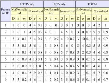
e ranges from 0.0 to 10.0 by an increment step of 1.0. For each feature subset, Table 8 presents the parameter values of SVM-K1 that produce best results.

Table 8. SVM-K1 Hyper-parameters values for HTTP-only, IRC-only, and TOTAL

Feature set ID

NotNormaliz

ed Normalized

NotNormali

zed Normalized

NotNormaliz

ed Normalized

D e m D e m D e m D e m D e m D e m

1 3 0 0 4 4 0.3 3 0 0 3 0 1 3 0 0 4 2 1

2 3 0 1 4 5 0.9 4 0 1 4 5 0 3 0 0.7 5 5 0.9

3 3 4 0.1 3 4 0.7 3 0 0.9 4 10 0.7 3 10 0.1 3 5 0.7

4 3 5 0.1 5 6 1 3 4 0.8 3 6 0 3 4 0.3 5 5 0.9

5 3 3 0.1 4 8 0.8 3 0 0.8 5 7 0.8 3 2 0.3 4 6 0.8

6 4 0 0.9 4 10 0.1 5 2 0.4 3 0 0.9 3 0 0.1 5 6 0.8

7 3 0 0.9 5 10 0 5 5 0.4 4 6 0.4 5 0 0.1 4 6 1

8 4 0 0.4 5 9 0.3 3 1 0.1 3 0 0.9 3 1 0.1 5 7 0.6

9 3 3 0.2 4 6 1 4 2 0.2 3 5 0.6 3 5 0.1 4 6 0.7

• SVM-K2 (radial basis function- RBF- kernel):

K(Xi,Xj) = exp(−γ||Xi − Xj||2),γ >0

SVM-K2 has two parameters:

1. regularization cost – C, we test C asC = 1 × 10e _,_where

e ranges from 0.0 to 10.0 by an increment of 1.0.

2. γ : scaling factor of Gaussian exponential function, we test in the range from 0.0 to 1.0 by an increment of 0.1. (if γ = 0, Weka use it as γ = 1/number of features) For each feature subset, Table 9 presents the parameter values of SVM-K2 that produce best results.

Table 9. SVM-K2 Hyper-parameters values for HTTP-only, IRC-only, and TOTAL

Feature set ID

NotNormali

zed Normalized

NotNormaliz

ed Normalized

NotNormaliz

ed Normalized

e γ e γ e γ e γ e γ e γ

1 1 0 6 0 0 0 1 0.5 1 0 3 0.6

2 1 0.1 7 0.3 1 0.1 8 0.5 1 0.1 7 0.7

3 1 0.1 3 0.5 1 0.1 3 0.4 1 0.1 6 0.1

4 1 0.1 10 0.7 1 0.1 8 0.3 1 0 6 0.9

5 1 0.1 6 0.4 1 0.1 8 0.3 1 0.1 6 0.7

6 1 0.1 7 0.9 1 0.1 9 0.9 1 0.1 8 1

7 1 0.1 10 1 1 0.1 7 0.1 1 0.1 10 1

8 1 0.1 8 0.9 3 0.1 6 0.9 4 0.1 7 1

9 3 0.1 5 1 1 0.1 3 0.5 1 0.1 6 0.8

5.4. Model Creation

After getting the optimized hyper-parameter values for both J48 and different SVM kernels, the next step is to create the detection model using those hyper-parameters by experimenting with each candidate feature set. The final objective is to determine which feature subset produces best detection results.

During parameter selection step, an initial model is already created with 5-fold cross-validation (CV) performance estimation. In 5-fold cross-validation (CV), the training dataset (malicious + benign) is randomly partitioned into 5 equal size datasets. Each dataset is used once to validate the model that was created using the remaining 4 datasets. Then, all 5 F1-measure values are combined in a single value that is used in hyper-parameter optimization as described in next section. In addition to the above splitting mechanisms, which is completely random, we applied two other mechanisms (combination and split 64-36%) to split the malicious dataset between training and validation phase:

•

In combination mechanism, traces from two botware families (IRC or/and HTTP) are used in training phase and the third family is kept for validation. For example, in HTTP-only model, if the two families (Blackenergy and Zeus) are used in training phase, Vertexnet family will be used in validation phase. This step is repeated for all family pairs, and then a combined F1-measure is calculated from F1-measure of all combinations. We can consider the combination mechanism as a concrete partitioned 3-fold cross-validation. The advantage of this method is to ensure that our model is more generic and independent on botware families.

(9)

for training and the other %34 dedicated for validation. The advantage of this method is to ensure that the detection model is more generic and independent on botnet configuration because each run of the botware sample is different from the others with regard to botnet and network configuration.

5.5. Model Selection

In our experiments, we create three different models to detect HTTP-based botnet (HTTP-only), IRC-based botnet (IRC-only) and both HTTP and IRC botnet (TOTAL). For each of these models, there are 18-candidates features subsets (9-normalized features subsets + 9-not (9-normalized features subsets). For each of these features subset, we applied the three split mechanisms (Cross Validation-CV, Combination, and split 66%-34%) to divide the dataset between training and validation phase. As mentioned before, we use J48 and three different kernels in SVM as machine learning algorithm. The goal now is to answer the question of which is the best performing feature-subset with which model and

which machine learning algorithm?.

As explained earlier, the botnet dataset is an imbalanced dataset where the number of positive instances is far less than the number of negative instances. F1-measure is a trade off between Precision and Recall metrics to assess the detection quality. It is recommended as a performance metric for such imbalanced datasets [46]. However, in our case, there are three different F1-measure values coming form Cross Validation, Combination, and split 66%-34% results. Therefore, we need a method to combine or average these different values. There are mainly two methods for this purpose; either by calculating the micro-average or the macro-average.

• Micro-average Method: we first calculate the total of TP, FP, and FN which are the summation of their values for different datasets (or folds). Then calculate F1-measure using the formula in Equation (4):

Eq. (4)

• Macro-average Method: Instead of calculating F1-measure based on overall TP, FP and FN, we calculate the F1-measure for different datasets (or folds), Equation (5). Then, we take the average of these F1-measures, Equation (6):

Eq. (5)

Eq. (6)

Based on previous research in [47], [48], the micro-average method is less biased and more precise than the macro-average method for equally sized datasets (or folds). Therefore we decided to use the micro-average method in 5-fold

cross-validation and combination mechanisms. Then to equally weight the results from all experiments (i.e., cross-validation, combination, and split 66%-34% mechanisms), the macro-average method is used to calculate a single F1-measure for the whole experiment. This single value of F1-measure will be the performance metric upon which we can determine the best model created over 18 feature subsets using J48 and three different SVM Kernels.

The final output of model selection process is three models for HTTP-only, IRC-only and TOTAL. These models will be integrated into BoTCap as explained in next section. To evaluate the performance of BoTCap, we test these models using the unseen dataset that was described in Section 5.1 (i.e., neither used in training nor in hyper-parameter optimization phase).

5.6. Implementation

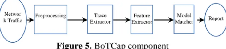
In this section, we present a prototype of BoTCap detection system that we implemented in Python. BoTCap is designed and implemented to detect local infected hosts by comparing a set of statistical features, extracted per trace, through a pre-trained machine learning model. As shown in Figure 5, BoTCap consists of four main components: Preprocessing, Trace Extractor, Feature Extractor, and Model Matcher.

Figure 5. BoTCap component

Preprocessing: The input for BoTCap is a network traffic capture that normally consists of a wide range of internet protocols. Preprocessing module filters out botnet-irrelevant traffic and keeps only TCP and UDP traffic.

Trace Extractor: the captured traffic is in the form of sporadic packets. BoTCap reassembles flows from the captured packet data. After that, it aggregates the flows that have the same 3-tuple (SrcIP, DstIP, DstPort) as a trace. Feature Extractor: For each trace, a set of statistical features are extracted. Feature extraction is performed in three steps. Firstly, it extracts statistical features per flow using Argus (Audit Record Generation and Utilization System) [49]. After that, we calculate the features in Table 1 per trace based on the trace's flows. Regarding the periodicity features (Table 2), we modified CAPTCP [50] to be applicable for both TCP and UDP traffic. It calculates the throughput of the up-link traffic. Then, it extracts the periodicity features using the algorithm described in (Code 1). The output of feature extractor is represented as a vector of features.

Model Matcher: To check whether a trace is a botnet trace, BoTCap compares the trace's vector of features to HTTP-only, IRC-only or TOTAL models. If the trace matches any model, BoTCap produces a detailed report that includes the internal host IP (bot) that produced this trace and the remote server IP which may be the C&C server of centralized botnet or another bot in the P2P botnet.

6. Results and Discussion

In the first part of this section, we report and discuss the output of model selection step. After that, we evaluate the

Networ

k Traffic Preprocessing Extractor Trace Report Feature

Extractor

(10)

performance of BoTCap using the test dataset. The results of the evaluation step will be reported in the second part.

6.1. Model Selection Results

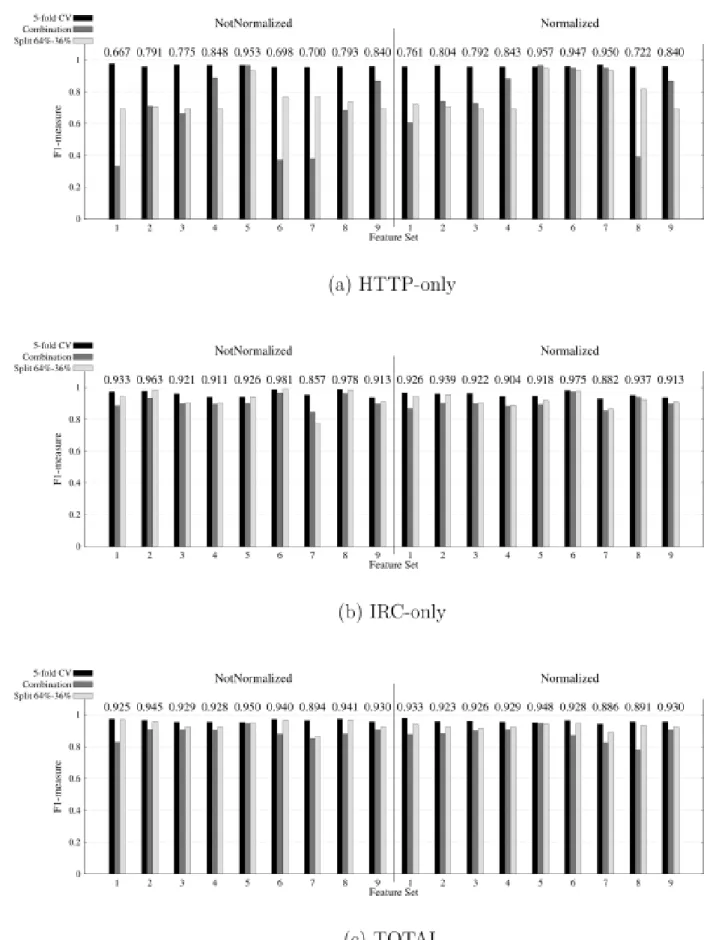
The next sets of figures present a histogram of F1-measure values calculated as described in Section 5.5. In each figure, the X-axis represents the ID of the feature set that were presented in Table 5. In the left half (NotNormalized), it shows the absolute values of the features while the right half (Normalized) shows the normalized values of the features. The columns of the histogram corresponds to F1-measure values for 5-fold CV, Combination, and split 64-36 respectively. Numbers in the top of the columns present the macro-average of F1-measure values as calculated by Equation (6).

6.1.1. J48 Algorithm

Figures I-(a, b, c), in Appendix A, display J48 results for HTTP-only, IRC-only and Total respectively. In Figure I-(a), we notice that the feature set with ID (5)-Normalized produces the best results (i.e., Highest F1-measure). When we examine the results of IRC-only shown in Figure I-(b), we find that feature set with ID (6)-NotNormalized has the highest F1-measure value. Finally, the results of TOTAL, indicates that feature set with ID (5) – NotNormalized has the highest F1-measure value, Figure I-(c). Over all, we observed that J48 results have more variations between the different feature sets in the case of HTTP-only regardless of being normalized or not where combined F1 measures (macro average) ranges from 0.667 to 0.957. By contrast, almost all J48 results of the IRC-only are more than 0.85 whereas all TOTAL results are approximately near 0.9.

6.1.2. SVM-K0

Figures II-(a, b, c) display the results obtained from SVM-K0 algorithm “linear kernel”. As shown in Figure II-(a), HTTP-only detection models using feature sets with IDs (2, 6, 7) – NotNormalized have the highest and the same value of F1-measure (0.903). By reference to Table 5, feature set-6 is subset from set-2 and set-7 is subset form set-6. We believe that is the reason why three sets give the same F1-measure value. This also means that the set with smallest number of features eliminates the need for extra features in the other two sets that seem to be redundant and have no effect. Therefore, we select feature set with ID-7-NotNormalized. Referring to Figures II-(b) and II-(c), the normalization process generally enhances the performance of IRC-only and TOTAL detection models. In IRC-only normalized feature set, F1-measure starts from 0.625 up to 0.958 but the highest F1-measure value 0.972, using feature set with ID (1)-NotNormalized. In TOTAL model, feature set with ID (1)– Normalized has the highest F1-measure value.

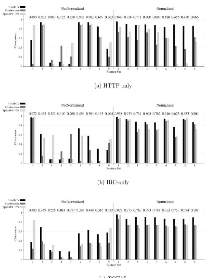
6.1.3. SVM-k1

As shown in Figures III-(a, b, c), the normalization process have a significant impact on the performance of the models that use SVM-K1 algorithm “polynomial kernel”. As shown in Figure III-(a), all feature sets that are Normalized, for HTTP-only models have more than 0.60 F1-measure value. Despite that the macro-average of F1-measure for 5-fold CV, Combination and split experiments in some sets such as sets (1, 3, 6, 8) can reach more than 0.75, but the result of the three experiments are not consistent. Feature set with ID-5 –

Normalized produces the highest and more consistent F1-measure (0.947) for HTTP-only. Referring to Figures III-(b) and III-(c) respectively, feature set with ID (1) – Normalized have the highest F1-measure (0.993) for IRC-only and feature set with ID (5) – Normalized have the highest F1-measure (0.941) for TOTAL model.

6.1.4. SVM-k2

Figures IV-(a, b, c) illustrate the results of using SVM-K2 algorithm “radial kernel”. Like SVM-K1, the normalization process have a significant impact on the performance of the models that use SVM-K2 algorithm. As shown in Figures IV-(a), and IV-(c), feature set with ID (5)–Normalized has the highest F1-measure value for HTTP-only model (0.937) and for TOTAL model (0.951) respectively. In Figure IV-(b), the model that uses feature set with ID (1)- NotNormalized cannot classify correctly any actual IRC malicious trace as a positive class “malicious class”. In contrast, the same feature set with ID (1) but 'Normalized' produces the highest F1-measure (0.997) for IRC-only.

6.1.5. Final Selection

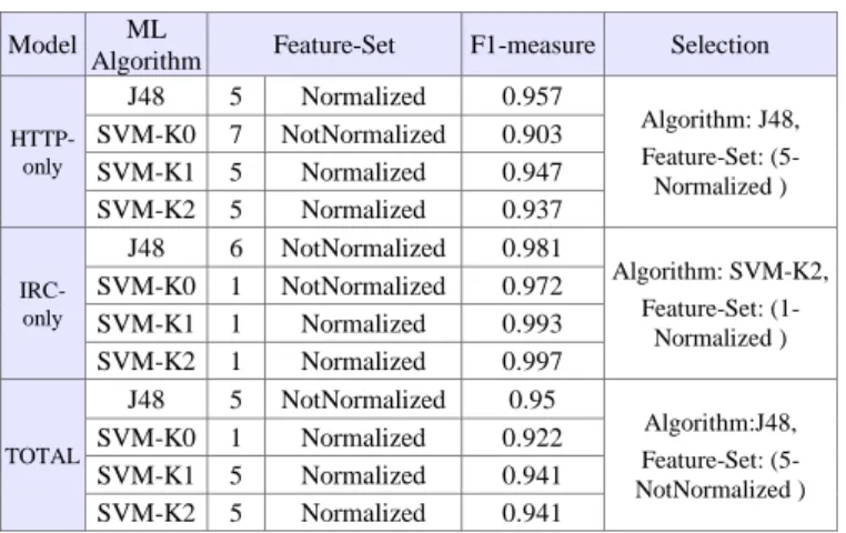
Table 10 summarizes the results that leads to answer the first part of the question that was raised in Section 5.5, “which is the best performing feature-subset?”. The remaining part of the question is which ML algorithm gives the highest detection performance? In order to be integrated in BoTCap.

As shown in Table 10, both J48 and the three different kernels of SVM are performing well in terms of F1-measure. Therefore, a good compromise is to combine these ML algorithms in multi-stage detection (voting majority rule or weighted models) or simply pick up the one that gives the highest performance; as we did hereafter in “Selection” column.

Table 10. Summary of Model Selection Model _AlgorithmML Feature-Set F1-measure Selection

HTTP-only

J48 5 Normalized 0.957

Algorithm: J48, Feature-Set: (5- Normalized )

SVM-K0 7 NotNormalized 0.903

SVM-K1 5 Normalized 0.947

IRC-only

J48 6 NotNormalized 0.981

Algorithm: SVM-K2, Feature-Set: (1-

Normalized )

SVM-K0 1 NotNormalized 0.972

TOTAL

J48 5 NotNormalized 0.95

Algorithm:J48, Feature-Set: (5- NotNormalized )

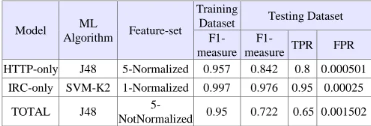
6.2. BoTCap Evaluation result

(11)

benign traces that are classified as malicious. TPR and F1-Measure are already defined by Equations (2 and 3), while FPR is defined in Equation (7):

Eq. (7)

As shown in Table 11, BoTCap can achieve 80% TPR with 0.05% of FPR in HTTP botnet detection, and 100% TPR with 0.025% of FPR in IRC botnet detection. Regarding the TOTAL model, it achieves 65% TPR with 0.15% FPR, which is an acceptable performance in botnet detection research field.

Table 11: BoTCap performance

Model _AlgorithmML Feature-set

Training

Dataset Testing Dataset

F1-measure

F1-measure TPR FPR

HTTP-only J48 5-Normalized 0.957 0.842 0.8 0.000501

IRC-only SVM-K2 1-Normalized 0.997 0.976 0.95 0.00025

TOTAL J48 _{NotNormalized}5- 0.95 0.722 0.65 0.001502

It is worth to note that we have also evaluated our BoTCap against a portion of CTU dataset that contains botnet traffic [51]. CTU-10 was selected for two reasons: Firstly, it is well described and annotated bot-C&C trace and secondly the number of bots and duration of traffic are satisfying our conditions (more than one bot and duration ~ 6 Hours). Unfortunately, after using the dataset as it is, BoTCap gets 100% FNR. By analyzing the CTU-10 dataset, we discovered the bad detection result is due to the fast-flux domain communication. This why the traffic between each bot and the C&C server was extracted in separate traces and are not included in the same trace. Having a closer look into the evaluation dataset revealed that the scenario of the dataset creation experiment contains 4 runs (i.e., start-up/shutdown actions) of the VMs. The duration of the first run is one and half hour while the other three runs are less than one hour. Besides that, the C&C url "irc.freenode.net" is resolved by DNS query every time the VMs start-up. Therefore, each start-up C&C url is resolved with a different IP which creates new trace. Consequently, the duration of extracted traces between each bot and C&C server are:

• one and half hour (only 4 traces) ==> Is_periodic = 0: not periodic due to std of freq. more than 10% of the freq.

• less than one hour (other 40 traces) ==> Is_periodic = -2: not periodic due to duration.

In what concerns the fast-flux communication where bots can be assigned several varying IPs instead of having fixed IPs. In this case, bots do not connect to known IPs but rather they connect to domain names that can be mapped to frequently changing IPs. This can deceive botnet detection systems because each time the bot connects to C&C using different IP. We solved this problem by identifying the trace in term of "Source IP, Destination domain instead of Destination IP, Destination Port" and the Destination domain can be resolved to one or more IPs. The procedure that implements fast-flux complements the main BoTCap analysis. It extracts DNS queries and arrange results in a dictionary. Then, it creates the flows using dest. IPs (as before) but while doing reverse lookup for each dest. IP in DNS dictionary. If there is a dest. domain matching the dest. IP, replace the dest. IP by the dest.

domain in flows. Otherwise, it keeps the dest. IP as it is and BoTCap continues its normal routine.

Accordingly, BoTCap algorithm and code was modified to overcome fast-flux technique where the results given in Table 11 are produced by the improved BoTCap.

7. Conclusion and Future work

This paper, presents our approach for machine learning-based botnet detection and its implementation (BoTCap). It aims to detect individual bots based on ML algorithm by using a set of distinctive statistical features extracted per trace.

During our research we have met several problems. The lack of botnet datasets, the lack of botware samples, fast-flux and encrypted botnet communications are just examples of challenging problems in botnet research. We have partially solved the botnet dataset problem by creating our own. We have deployed and operated some botnet samples locally within our laboratory. However, this solution is effort consuming as we should find botware samples from the wild and be able to render it functional, which is intrinsically difficult. This was obvious in the dataset that we have constructed, which does not contain peer to peer datasets because we couldn’t find functioning P2P botware samples during the research time window. This is the main reason why we decided to focus on centralized botnets (IRC and HTTP). Another shortcoming of the dataset is that it does not cover the latest trends in botnet communications. For example, employing social networks such as Facebook and Twitter as communication channels between bots and C&C. Regarding the encrypted traffic, we argue that the statistical-based trace feature can solve this problem where the detection is independent of traffic contents, which was verified by including encrypted botnet traffic in the dataset (both learning and testing datasets).

We addressed all ML approach steps to find the set of features that give the highest F1-measure using J48 and three different kernels of SVM. A botnet dataset was created in laboratory from real botware samples of two types: HTTP and IRC. Based on this dataset, separate ML models were created: HTTP-Only, IRC-Only and TOTAL that contains both http and IRC. The models were tested against a “foreign” dataset: CTU-10. Unfortunately, it showed some glitches related to fast-flux problem. Accordingly, we modified the trace extraction part in BoTCap to be able to deal with botware that employ fast-flux. Then the trained ML models were integrated in a tool called BoTCap.

The results showed that our tool can detect bot infections with high detection rates up to 80% and 95 % for HTTP and IRC based botnet respectively and very small false positive rates of nearly 0.05% and 0.025% respectively.