AbstractThis paper discusses data mining applications, especially the use of support vector machines to identify a fault in the 13 nodes radial distribution system of IEEE standard. The identification process was carried out with support vector machine (SVM). Prior to the identification process by SVM, feature extraction was carried out using wavelet transformation for signal decomposition and signal size reduction. To determine the performance of the identification, ROC (Receiver Operating Characteristic) analysis was used. Based on the curve formed by the ROC a fault in the radial distribution can be identified by SVM with “good” performance This is indicated by the value of the best cut-off point is 0.8 and area under the curve is 0.85854.
KeywordsData mining, ROC, SVM, wavelet transformation, radial distribution systems.
I.INTRODUCTION
ault detection and diagnosis on power system is an important part in the management of distribution system. The information of fault on distribution system helps us to coordinate the security system [1].
Fault detection and diagnosis require recorded data from the network systems. There are three main sources of data: (1) field data, collected by various devices distributed through out the system, (2) centralized data archives, such as those maintained and controlled centralized by SCADA systems, (3) data from simulation to carry out planning or operational environment. Those data generally have a large volume (terabyte-sized) that requires special handling. To manage information based on data from the network system, Data Mining tools can be used [2].
Data mining is used to extract or ‖to mine‖ knowledge from large amounts of data. Data mining or referred as Knowledge Discovery from Data (KDD) is a process that contains a series of stages which include, (1) data cleaning, to remove noise and inconsistent data, (2) data integration, where multiple data sources may be combined, (3) data selection, where data relevant to the
1Dian Retno Sawitri is with the Department of Electrical
Engineering, Faculty of Industrial Technology, Dian Nuswantoro University, Semarang, Indonesia and student of Civil Engineering Doctorate Program Institut Teknologi Sepuluh Nopember, Surabaya, 60111, Indonesia.
2Arif Muntasa is with the Department of Informatics Technology,
Trunojoyo University, Kamal, Indonesia and student of Civil Engineering Doctorate Program Institut Teknologi Sepuluh Nopember, Surabaya, 60111, Indonesia.
3 Ketut Edi Purnama, M. Ashari, and Mauridhi Hery Purnomo are
with Department of Electrical Engineering, Faculty of Industrial Technology, Institut Teknologi Sepuluh Nopember, Surabaya, 60111, Indonesia.
analysis task is retrieved from the database, (4) data transformation, where data is transformed into forms appropriate for mining, (5) data mining, an essential process where intelligent methods are applied in order to extract data patterns, (6) Pattern evaluation, to identify the interesting patterns represented as knowledge based on some interesting measurement, (7) Knowledge representation, where visualization and knowledge representation techniques are used to present the mined knowledge to user [3].
Data Mining Applications in power systems can be used to predict the level of power system security. Security level can be predicted by determining whether an operation is running in a stable condition or not by identifying the occurrence of faults, including identifying the characteristics of fault [2].
Applications of data mining for fault detection and diagnosis on power system have been carried out. One of them is used to identify congestion problem in transmission planning. The methodology allows to identify not only the transmission paths and corridors which have congestion problems, but also the scenarios producing these critical situations [18]. Other methodologies used to identify fault on power system are wavelet analysis [6, 7, 8, 14, 15, 16], artificial neural networks [7], [14], and Support Vector Machine (SVM) [6, 7, 12, 17].
Wavelet transformation is generally used as a feature extraction before classification by neural network, SVM, or other methods [6, 7, 14, 16]. It is also used to determine the location of disruption [8] and to detect any disturbance signal based on the resulted signal [15].
Artificial neural network is used to recognize the existence of power quality disturbances after the previous signal extracted by wavelet [14] and the results are compared with SVM [7, 17].
The Use of SVM for power system disturbance classification was applied to distinguish the type of disturbance (sag, swell, harmonics, outage, sag with harmonics, swell with harmonics) [6], [7], and the voltage disturbance at the power network [12], [17].
This paper proposes fault identification and diagnosis on radial distribution system using wavelet-support vector machine. The previous research analysis indicated that SVM could recognize a disturbance with level of precision was 84.31% [20]. In this paper, research is continued with analyzes of new more data. After identified with wavelet-SVM, the data was analyzed by ROC (Receiver Operating Characteristics) to determine the classification performance. Based on ROC curve and confusion metrics, conclusion can be drawn.
The uses of ROC in most previous studies were applied to pattern recognition. Analyzed of the patterns
Data Mining Based Receiver Operating
Characteristic (ROC) for Fault Detection and
Diagnosis in Radial Distribution System
Dian Retno Sawitri
1, Arif Muntasa
2, Ketut Edi Purnama
3, M. Ashari
3, and Mauridhi Hery Purnomo
35are used to diagnose a disease [23, 24]. The ROC analysis for power system research up to now not was found. In this paper, the application of ROC analysis will be tested to examine the identified of fault on a radial distribution system.
A. Feature Extraction with Wavelet Transformation
Wavelet is mathematical functions that divide data into different frequency components, and then each component is studied with a resolution matched to its scale [4]. Wavelet transformation is used to represent a function with wavelet. The wavelet transformation provides information about the frequency of a signal similar to the Fourier Transformation (FT). Contrary to the FT, wavelet transformation is able to focus on short time intervals for high-frequency components and long time intervals for low-frequency components [5].
Wavelet transformation consists of Continues Wavelet Transformation (CWT) and Discrete Wavelet Transform (DWT) [5], [6], [7], [8]. The wavelet transform of continuous signal x(t) is defined as :
dt b a t t x a b a x CWT
* ) ( | | 1 ) , ( (1)where (t) is called the mother wavelet, the asterisk denotes complex conjugate, while a and b (a, b R) are scaling (dilation and translation). The scale parameter a
will decide the oscillatory frequency and the length of the wavelet and the translation parameter b will decide its shifting position.
Dilation and translation of mother wavelet can be replaced by selecting the value a = a0m and b = n.b0.a0m, the value of a0 and b0 are constant with a0 > 1, b0 > 0, m,
n, Z, and Z is the set of positive integer, so can be defined as :
m,n(t) = a0-m/2(a0-mt – n.b0) (2)
Discrete Wavelet Transformation DWT is defined as:
f t t dt
n m f
DWT ( , ) ( )m,n( )
(3)
Usually a0 = 2 and b0 = 1 are selected. The selection of
those values produces a dyadic-orthonormal wavelet
transform as a basis for multiresolution analysis (MRA).
In MRA, wavelet and scaling functions are used as building blocks to decompose and to construct the signal at different resolution levels [7]. A signal x(t) can be decomposed completely and in detail by scaling function
m(t) provided by wavelet m(t)[5], so m,n(t) and m,n(t) are defined as :
m,n(t) = 2-m/2(2-m/2t – n)
m,n(t) = 2-m/2 (2-m/2t – n) (4)
Scaling functions are associated with low-pass filters with coefficient {h(n), nZ}, while wavelet functions are associated with high-pass filters with coefficient {g(n), nZ}, (Fig. 1). Two level scaling filters produce:
) 2 ( 2 ) ( ) ( ) 2 ( 2 ) ( ) ( n t n g t n t n h t n n
(5)Some important characteristics of these filters are: 1.
( )21n
n
h and
n
n
g( )2 1 (6)
2.
( ) 2n
n
h and
n
n
g( ) 0 (7)
3. Filter g(n) is alternative flip of the filter h(n), which means there is an odd integer N so:
g(n) = (-1)n.h(N-n) (8)
Considering the filter bank implementation on Fig. 1. The relationship of the approximation coefficients and detailed coefficients between two adjacent levels is stated as :
) ( ) 2 ( )
(k h k ncA 1 n
cA
n
j
j
(9)
n
j j k g k ncA n
cD ( ) (2 ) 1( ) (10)
cAj and cDj represent the approximation and detailed coefficient of the signal level respectively.
In this way, the decomposition coefficient of MRA analysis can be described as:
[A0] [c.A1, c.D1]
[c.A2, c.D2, c.D1]
[c.A3, c.D3, c.D2, c. D1]
… (11)
Which correspond to the decomposition of signal x(t) as : x(t) = A1(t) + D1(t)
= A2(t) + D2(t) + D1(t)
= A3(t) + D3(t) + D2(t) + D1(t)
= ... (12)
Where Ai(t) is an approximation at level i and Di(t) is called the detail at level i.
To reduce the feature dimension, the energy is calculated for each level of decomposition as a new input variable for the classification of disturbance. Energy at each level of decomposition is calculated using the following equation: l i D ED N j ij
i | | , 1,2,...,
1 2
(13)
N j ij l A EA 1 2 | | (14)i = 1, 2, …, l is wavelet decomposition level from level 1 to level l. N is the number coefficient of details or the approximation at each level of decomposition. EDi is energy from details of decomposition level i and EAlis energy of the decomposition of the approximation at level l.
B. Support Vector Machine for Classification
Support vector machine (SVM) is a learning machine that is used to classify two groups of classes. The Machine conceptually implements the input vector which is non-linear mapping to high dimensional feature space [9].
SVM classification [10] is used to establish the optimal objective function f(x) that accurately classifies the data into two classes and minimizes misclassify-cation.
f(x)=sign(g(x)) (15)
This goal will be achieved using the method of structural risk minimization (SRM) in which the expected classification error (R) of the data is limited by the amount of training error rate [12].
N h N h N t R 4 ln 1 2 ln (16)
Where t is the number of learning error, N is the number of learning sample and is confidence intervals.
performance using SVM (Fig. 2). The function g(x) in equation (15) is the boundary function which is derived from a set of training sample.
X={x1, x2, …, xn}, x
M
(17)
Each training sample xi has M features describing a particular sign and belongs to one of two classes.
Y={y1,y2,…,yn}. Y {-1,1} (18) The boundary function comprises hyper plane
g(x)=w,x + b (19)
Where, w and b shall be derived in such a way that unseen data can be classified correctly. This is achieved by maximizing the margin of separation between the two classes. Based on [11], value of maximal margin can be formulated as a Quadratic Programming (QP) to optimize problems.
n i i C w w 1 2 || || 2 1 min ) ,( (20)
Subject to the constraint that all training samples are correctly classified (i.e., all training sample are placed on the margin or outside the margin), that is
yi(w,xi + b) 1- i, i = 1, …, n (21)
where i, i = 1, ..., n is non negative slack variable. By
minimizing the left hand side of equation of (20), the complexity of the SVM is reduced, and by minimizing the right side, the number of training error is decreased. Parameter C in (20) is a regularization parameter and is previously selected to be the tradeoff between the two sides in (20). The QP constrained problem defined in (20) and (21) is solved by introducing Lagrange multipliers i 0 and i 0 and the Lagrange function
n i i i i i n i i n ii y wx b
C w b w L 1 1 1 2 ] , [ { || || 2 1 ) , , , ,
( (22)
According to the theory of QP optimization, it is better to solve (22) by introducing the dual formulation of the problem
max min ( , , , , )
) , ( max , , , ,
W Lwwb b
(23)
Where, i and i are Lagrange multipliers. Which means
that the optimal solution is given by firstly minimizing
w, b, and and thereafter maximizing, paying respect to
i 0 and i 0. By substituting (21) into (22), the
problem can be transformed to its dual formulation given by
n i n i n j j i j i j i ia yy x x
1 1 1
, 2
1
max (24)
and shall be maximized by the constraints
iI = 0 and 0 < i < C for i = 1, …, n (25) vector w, has an expansion in terms of a subset of the training samples where the Lagrange multiplier i is non
zero. Those training sample will also meet the Karush-Kuhn-Tucker condition.
i{yi[w,xi+b]–1+i}=0, i=1,…,n. (26) Equation (26) states that only the training vectors correspond to non zero multipliers, the support vector (SVs), are needed to describe the hyperplane. In the case of linearly separable data, all SVs will lie on the margin and hence the number of SVs can be very small. Consequently, the decision boundary g(x) is determined by only using a subset of the training samples and the rest of the training samples are not needed
b x x y x g i N i i i
, ) ( 1 (27)Where x is the input test vector, x, xi is the inner
product, N is the number of support vector, and b is the
bias value.
In the case where a linear decision boundary is inappropriate, the SVM can map the input vector, x, to higher dimensional feature space [10], [11]. This is achieved by introducing a kernel function K(.,.) and substituting the following equation to (24).
x, xi K(xi,xj) (28)
Hence, it yields,
n i n i n j j i j i j i ia 1 2 1 1 y y K(x,x )
1
max (29)
and (29) shall be maximize under the constrain in (21) and the solution is provided by a software package for solving optimization problem. The decision boundary
g(x) in (27) is then modified by substituting x, xi with
K(xi, xj)
b x x K y x g i N i i i
) , ( ) ( 1 (30)Functions that satisfy Mercer’s theorem are useable as Kernel function. Soft decision SVM is then applied. Examples of such kernels are given in Table 1 [12].
C. Classification Performance Analysis
Classification performance can be analyzed by graph Receiver Operating Characteristic (ROC). ROC graph is a technique to visualize, organize, and choose the type of classification based on its performance [13].
Classification performance can be seen by confusion matrix. A classification model (classifier) is a mapping of instances into a certain class/group. In binary classification, the outcomes are labeled either as positive (p) or negative (n) class. There are four possible outcomes from a binary classifier. They are true positive,
false negative, true negative, and false positive (Fig. 3).
If the instance is positive and it is classified as positive, it is counted as a true positive; if it is classified as negative, it is counted as a false negative. If the instance is negative and it is classified as negative, it is counted as a
true negative; if it is classified as positive, it is counted
as a false positive.
The matrix in Fig. 3., shows a confusion matrix and equations of several common matrix that can be calculated from it. The numbers along the major diagonal represent the correct decisions made, while the numbers in this diagonal represent the errors—the confusion—between the various classes. The true positive rate (also called hit rate and recall) of a classifier is estimated as
positives Total classified correctly Positives rate
tp (31)
The false positive rate (also called false alarm rate) from classifier is :
negatives Total classified y incorrectl Negative rate
fp (32)
Additional terms associated with ROC curves are:
Sensitive = recall (33)
negatives True positives False negatives True y specificit
Positive predictive value = precision (35)
D. ROC space
Based on confusion metrics, ROC curve can be made. ROC curve is a two-dimensional graph, where Y axis expresses tp rate and X axis expresses fp rate. ROC graph illustrates the relationship between the relative profits (true Positives) and costs (false Positives). Fig. 4. shows the ROC graph with the class labeled A to E.
The best possible prediction method would yield a point in the upper left corner or coordinate (0,1) of the ROC space, representing 100% sensitivity (no false negatives) and 100% specificity (no false positives). The (0,1) point is also called a perfect classification. A completely random guess would give a point along a diagonal line (the so-called line of no-discrimination) from the left bottom to the top right corners.
The diagonal line divides the ROC space in areas of good or bad classification/diagnostic. Points above the diagonal line indicate good classification results, while points below the line indicate wrong results (although the prediction method can be simply inverted to get points above the line).
E. Curve in ROC space
Discrete classification such as decision tree or rule sets usually produces numerical values or binary labels Y and N. For other types of classification such as Naive Bayes
or neural network usually produce a probability value or
score. To determine a point in ROC space for the probability value is usually by determining the threshold value, for example, if the probability value> 0.5 then Y and if the probability <= 0.5 then the N. In this way the point position in the ROC space can be determined. Placement of points according to the threshold would produce a ROC curve.
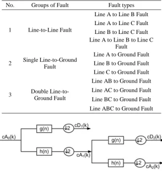
The data which would be analyzed was raised with Matlab Simulink. Fault was generated on node 650 with various types (i.e. line-to-line fault, single line-to-ground fault, and double line-to-ground fault) [1]. Total class fault is 11 (Table 2).
The Fault effect at bus 650 was recorded on other nodes. The recorded signal was the ABC signals. Signal was converted into dq0 signal, before extracted by wavelet transformation. The result of wavelet transformation was a feature extraction which was then classified by support vector machine (SVM). SVM classification results were then tested its performance by ROC analysis. The result was analyzed further to determine the mining of the analysis results.
III.RESULT AND ANALYSIS
A. Result of Wavelet Feature Extractions
Feature extractions performed with wavelet transformation based on the signals have been raised. The results of feature extraction would produce a clearer signal with smaller dimensions making it easier to be classified. Examples of initial signal and signal decomposition results are illustrated in Fig. 7.
Results of the wavelet decomposition were the ABC signals which were transformed into a signal "dq0". Fig. 7 (a), (b), and (c) show the decomposition results for each signal. Respectively, the process of decomposition performed on all existing signals. The results of this
wavelet decomposition would then be identified with support vector machine (SVM).
B. Fault Identification with SVM
The results of feature extraction with wavelet transformation were then identified using a Support Vector Machine (SVM) which was built with Matlab. The number of classes to be identified was 11 (Table 2) and each class had 13 data measured from each node that existed. Out of the thirteen data, some were used as training data (2 to 5 data) and the rest were used as testing data. Strategy used for classification was the "One Against One (OAO)" [21], [22]. This strategy was done by SVM classification for each class. If there were k classes there would be k (k-1) / 2 SVM which would be trained to distinguish samples from a class from one sample from another class. Usually, the classification of an unknown pattern was determined based on the maximum voting, where each SVM would choose a class.
To test the SVM program which had been made, experiments were conducted with randomly selected sequence of data to be trained and the data to be tested. Supposing that out of the 13 existing data, data 1and 2 were selected as training data and the rest was testing data. Results of identification with the data would indicate how much data from each class could be identified. The experiment was repeated 32 times for different data sequences.
Based on the experimental results, average of 95.01% data with a standard deviation of 4.71 was identified. This shows that SVM can identify the fault in the existing distribution system.
Performance of the classification results for each class can be seen in Table 3. It shows, that each class can be identified well by SVM. The lowest identification was in Class 9 (AC Line to Ground fault). Meanwhile, other classes were identified above 85% and some even reached 100%. This shows that the SVM can identify the faults on the radial distribution system properly.
C. Data Mining based Receiver Operating
Charac-teristics (ROC).
Receiver Operating Characteristics (ROC) is one of the methods in data mining. Data mining is suitably applied to detect faults in power systems distribution because it involves real time and large data. ROC graphs are useful for organizing classifier and visualizing their performance. The combination of SVM and the ROC are well suited to detect interference with the power system distribution. With the ROC will be determined whether the SVM classifier has good performance.
With ROC analysis, the value of true positive rate, true negative rate, false negative rate and false positive rate (Fig. 8) and area under the curve ROC (AUC) would be determined. The results of the analysis is presented in the ROC curves and contingency tables.
The table in Fig. 8 is presented in graph in Fig. 9 to determine the percentage of each value, while classification performance calculations are presented in Table 5.
and the probability test is negative for classes that are not known = 0.983. The level of accuracy is 0.7661 that means error rate is 22.25%. Precision value of 0.9878 indicates the probability that the class is recognized when the test is positive
The result of ROC analysis can also be described in the ROC graph so that Area Under Curve ROC graph (AUC) can also be calculated as shown in Table 6.
TABLE 1.EXAMPLE OF KERNEL FUNCTIONS
Kernel Types Functions
Polynominal K(x,y)=(x.y+)d
Radial Basis Function (RBF) | |2
) ,
(x y e yxy
K
Sigmoidal K(x,y)=tanh(K.(x.y)-)
TABLE 2.TYPE OF FAULT IS GENERATED BY SIMULINK
No. Groups of Fault Fault types
1 Line-to-Line Fault
Line A to Line B Fault Line A to Line C Fault Line B to Line C Fault Line A to Line B to Line C
Fault
2 Single Line-to-Ground Fault
Line A to Ground Fault Line B to Ground Fault Line C to Ground Fault
3 Double Line-to-Ground Fault
Line AB to Ground Fault
Line AC to Ground Fault
Line BC to Ground Fault Line ABC to Ground Fault
Fig. 1. Two levels filter bank wavelet analysis
Fig. 2. Optimal separating hyper plane
Fig. 3. Confusion matrix and common performance matrix calculated from it
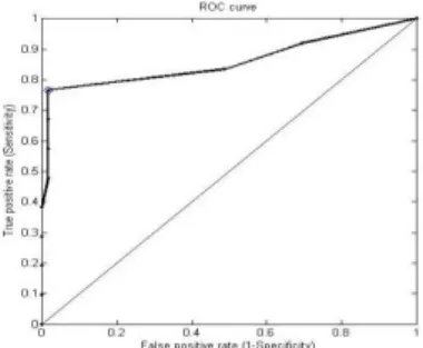
Analysis results in Table 6 stated that the area under the curve (AUC) was 0.85854 with standard error of 0.01021, while the value of confidence interval (95%) was in the range of 0.83853 - 0.87856. Value cut-off point for the best sensitivity and specificity values are marked by 8.00, the blue circle (Fig. 10.). Based on the area under the curve of 0.85854, the resulting classification performance, "SVM" can be classified as "good". Classification performance can also be described in the precision-recall graph (Fig. 10).
TABLE 3.IDENTIFICATION RESULT FOR EACH CLASS
Class Identified No Identified
Strength
(%)
1 304 0 100
2 304 0 100
3 304 0 100
4 304 0 100
5 301 3 99.01
6 304 0 100
7 304 0 100
8 304 0 100
9 220 84 72.37
10 269 35 88.49
11 259 45 85.2
Total 3177 167 95.01
TABLE 4.ANALYZE PERFORMANCE OF ROC
No Variable Value
1 FP rate 0.017
176 3
2 TP rate =
recall 3168 0.7661
2427
3 Precision 0.9878
3 2427
2427
4 Accuracy 0.7775
176 2427
173
2427
TABEL 5.AREA UNDER CURVE ROC(AUC)
AUC
SError 0.95 Confidence
Interval
0.85854 0.01021 0.83853 0.87856
Standardized AUC 1-tail p-value
35.1083 0.000000
The area is statistically greater than 0.5
Fig. 5. Fault detection and diagnosis block diagram in this study
Fig. 6. IEEE 13 Nodes radial distribution tes feeder
TABLE 6.AREA UNDER CURVE ROC(AUC)
AUC SError 0.95 Confidence Interval
0.85854 0.01021 0.83853 0.87856
Standardized AU 1-tail p-value
35.1083 0.000000
The area is statistically greater than 0.5
Fig. 7.a. Example of feature extraction of signal d
Fig. 7.b. Example of feature extraction of signal q
Fig. 7.c. Example of feature extraction signal 0
TP = 2427 FP = 3
FN = 741 TN = 173
p n
Y
N
True Class
H
y
p
o
th
e
s
iz
e
d
C
la
s
s
Column Total P=3168 N=176
Fig. 8. Confusion matrix of fault identification in radial distribution system
Fig. 10. ROC Graph for fault identification
Fig. 11 notes that the precision value increases if the value of recall (True Positive Rate) is also increased. The rate of precision values above 8.0 (Table 5) indicates the performance of the classification is ―good".
IV.CONCLUSION AND FUTURE WORKS
Support Vector Machine can be used to identify the occurrence of faults in power system, especially the radial distribution system properly. The addition amount of data that are identified can improve the performance of identification. In the previous study with 10 replications of data for each type of fault identification, score of 84.31% was obtained. By adding data from 10 to 13, level of recognition rises to 95.01%. The use of wavelet transformation as feature extraction will cause the signal more easily recognizable
ROC analysis showed that the classification performance was "good", This is shown by the ROC graph in which all points are above the boundary line y = x. In addition, the value of the area under the curve (AUC) was 85.85% showing that the classification performance was in good categories.
In the future identification using wavelet-SVM-ROC will be applied to other plant, among others is to detect faults on the electricity network in a building and the HVAC (Heating, Ventilation and Air Conditioning) system.
REFERENCES
[1] H. Saadat, 1999, ―Power system analysis‖, Mc-Graw Hill Int. Singapore.
[2] C. Olaru, P. Geurts, and L. Wehenkel, 1999, ―Data mining tools and application in power system engineering‖, Proceedings of the 13th Power System Computation Conference, PSCC99, page 324-330 - june 28-July 2nd.
[3] J. Han and M. Kamber, 2006, ―Data mining‖, Concept and Techniques, 2nd Ed., Morgan Kaufman Publisher.
[4] A. Graps, 1995, ―An introduction to wavelet‖, IEEE Computational Science and Engineering, Summer, vol. 2, num. 2.
[5] M. Karimi, H. Mokhtari, and M. R. Iravani, 2000, ―Wavelet based on-line disturbance detection for power quality applications‖, IEEE Transaction on Power Delivery, Vol. 15, No. 4, October.
[6] Haibo, 2006, ―A self organizing learning array system for power quality classification based on wavelet transform‖, IEEE Transaction on Power Delivery, Vol 21, No. 1, January. [7] S. Ekici, 2009, Classification of power system disturbance using
support vector machine, Expert Systems with Application, pp. 36.
[8] A. Borghetti, M. Bosetti, M. Di Silvestro, C.A. Nucci, and M. Paolone, 2007, ‖Continuous-wavelet transform for fault location in distribution power networks : Definition of mother wavelet inferred from fault originated transients‖, The International Conference on Power Systems Transients, Lyon, France, June 4-7.
Fig. 11. Precision – recall graph
[9] C. Cortes and V. Vapnik, 1995, ―Support Vector Network‖,
Machine Learning, 20, pp. 273-297.
[10] V. N. Vapnik, 1998, Statistical learning theory. New York: Wiley.
[11] N. Cristianini and J. Shawe-Taylor, 2000, An Introduction to Support Vector Machines. Cambridge, MA: Cambridge Univ. Press.
[12] P. G. V. Axelberg, Irene Yu-Hua Gu, and M. H. J. Bollen, 2007, ―Support vector machine for classification of voltage disturbance‖, IEEE Transaction on Power delivery, Vol. 22, No. 3, July.
[13] T. Fawcett, 2006, ―An introduction to ROC analysis‖, Pattern Recognition Letters, 27, pp 861 – 874.
[14] S. Santoso, E. J. powers, W. M. Grady, and A. C. Parsons, 2000, ―Power quality disturbance waveform recognition using wavelet based neural classifier part I: Theoretical foundation‖, IEEE Trans. Power Del., vol. 15, no. 1, pp. 222–228, Jan.
[15] Mokhtari, H. M. K. Ghartemani, and M. R. Iravani, 2002, ―Experimental performance evaluation of a wavelet-based on-line voltage detection method for power quality application”, IEEE transaction on Power Delivery, Vol. 17, No. 1, January. [16] T. K. Galil, 2004, ―Power quality disturbance classification
using the inductive inference approach‖, IEEE Transaction on Power Delivery, Vol. 19, No. 4,October.
[17] L. S. Moulin, A. P. A. da Silva, M. A. El-Sharkawi, and R. J. Marks, II, ―Support vector machines for transient stability analysis of large-scale power systems‖, IEEE Trans. Power Syst., vol. 19, no. 2, pp. 818–825, May.
[18] E. F. Sanchez-Ubeda, J. Peco, P. Raymont, T. Gbrnez, and S. Baiiales, A. L. Hernhdez, 2001, ―Application of data mining techniques to identify structural congestion problems under uncertainty‖, PPTIEEE Porto Power Tech Conference 10th -13th September, Porto, Portugal
[19] IEEE Distribution Planning Working Group Report, 1991, ―Radial distribution test feeders‖, IEEE Transactioinson Power Systems,, August, Volume 6, Number 3, pp 975-985.
[20] D. R. Sawitri, A. Muntasa, M. Ashari, and M. H. Purnomo, 2009, ―Identifikasi gangguan sistem distribusi radial berbasis wavelet-support vector machine‖, Proceeding of Conference on Information Technology and Electrical Engineering (CITEE),
August 4.
[21] J. Milgram, M. Cheriet, and R. Sabourin, ―One against one or one against all‖: Which One is Better for Handwriting
Recognition with SVMs?,
www.livia.etsmtl.ca/publications/2006/MILGRAM_IWFHR_20 06.pdf.
[22] J. Milgram, M. Cheriet, and R. Sabourin, 2007, ―Image classification using SVMs : One–Against-One Vs One-Against-All‖, Proccedings of the 28th Asian Conference on Remote Sensing.
[23] X. He, X. Song, and E. C. Frey, 2008, ―Application of three-class ROC analysis to task-based image quality assessment of simultaneous Dual-Isotope myocardial perfusion SPECT (MPS)‖, IEEE Transaction on Medical Imaging, Vo. 27, No. 11. Nopember.