Implementation of the Unified Post Processor (UPP) and the Model Evaluation Tools (MET) for WRF-chem evaluation performance

(1)

Implementation of the Unified Post Processor (UPP) and the Model

Evaluation Tools (MET) for WRF-chem evaluation performance

Agustín GARCÍA-REYNOSO * and Marco A. MORA-RAMÍREZ

Centro de Ciencias de la Atmósfera, Universidad Nacional Autónoma de México, Circuito de la Investigación

Científica s/n, Ciudad Universitaria, 04510 Ciudad de México

*Corresponding author; email: [email protected]

Received: October 14, 2016; accepted: March 16, 2017

RESUMEN

Este trabajo se centra en la descripción detallada de varias modificaciones realizadas a las versiones más

recientes de los paquetes informáticos Unified Post Processor (UPP) y Model Evaluation Tools (MET), las

cuales son necesarias para incorporar especies químicas importantes y parámetros meteorológicos al proceso

de verificación. Los cambios realizados en ambos programas se ejemplifican con un episodio de altas

con-centraciones de ozono, comparando simulaciones del modelo Weather Research and Forecasting-chemistry

(WRF-chem) con datos observacionales de la Red Automática de Monitoreo Atmosférico correspondientes

a un fin de semana en la Zona Metropolitana de la Ciudad de México. El modelo WRF-chem se alimentó

con datos formateados del Inventario Nacional de Emisiones (2006). Se proporcionan ejemplos de resultados

y gráficas que contemplan la adición de nuevas especies químicas al proceso de verificación, con el objeto

de explicar el tipo de mediciones de verificación y gráficas que el MET podría aportar en la actualidad. Por

último, las modificaciones realizadas a diferentes archivos de los paquetes UPP y MET podrían ser de interés

en particular para los usuarios y desarrolladores del modelo WRF-chem preocupados por el pronóstico o la

investigación de episodios con mala calidad del aire urbano.

ABSTRACT

This study focuses on a detailed description of several modifications made in both the Unified Post-Processor

(UPP) and the Model Evaluation Tools (MET) release packages, which are necessary in order to incorporate

relevant chemical species and meteorological parameters into the verification process. The changes made

in UPP and MET are illustrated with a high ozone concentration episode, comparing the Weather Research

and Forecasting-chemistry (WRF-chem) simulations against observational data from the Red Automática

de Monitoreo Atmosférico (Automatic Atmospheric Monitoring Network) during a weekend in the Mexico

City Metropolitan Area. National Emission Inventory (2006) formatted data was supplied to the WRF-chem

model. Examples of statistical results and plots contemplating the new chemical species added to the

verifi-cation process are given, with the aim to illustrate the kind of verifiverifi-cation measurements and plots that MET

could provide now. Finally, The modifications made over different files in UPP and MET packages could be

of particular interest for users and developers of the WRF-chem model concerned about the forecast of the

analysis episodes related with poor urban air quality.

Keywords:

WRF-chem, evaluation, UPP, MET.

(2)

1. Introduction

Improving air quality in many large cities requires a

better understanding of the sources and

transforma-tion of pollutants in the atmosphere. The air quality

models constitute a major tool to carry out this task.

However, the process of verifying the model results

can be even more important.

The Weather Research Forecast (WRF) model was

developed at the National Center for Atmospheric

Research (NCAR). Grell et al. (2005) and Fast et al.

(2006) updates incorporated into the WRF the chemical

transformations, complex gas-phase chemistry,

photol-ysis, and aerosols, creating in this way the WRF-chem

model. In order to work with the WRF-chem model

outputs, there are several computing packages: NCL

(NCAR, 2015); GrADS (COLA, 2015); NetCDF

(UNIDATA, 2015); and the Unified Post-Processor

(UPP), developed at NOAA (DTC, 2015). All of them

are very useful to visualize and extract information.

Also, there are statistical tools that serve to evaluate

the performance of model simulations, in some cases

comparing the simulation results against observations.

Recently, the Model Evaluation Tools (MET)

(Gotway et al., 2014), a state-of-the-art suite of

ver-ification tools, was released by the Developmental

Testbed Center (DTC) (http://www.dtcenter.org/met/

users/index.php). It can perform a set of standard

veri-fication scores by comparing gridded model data with

point-base observations and with gridded observations,

among others. This kind of software provides useful

information to the model users in order to improve

the model performance by testing different model

configuration setups, to improve the forecast and the

decision making, and to identify forecast weakness

and strengths. MET reads the output from UPP. In

turn, the UPP code take in WRF output files (wrfout*)

in NetCDF format. The original configuration of

UPP can read several fields (eg, U, V, T, albedo) (see

Baldwin

et al

., 2012, chapter 7, table 2). However, as

far as we have seen, the chemical species oriented to

the study of air quality are not included in these fields.

Therefore, changes were made in the UPP source code

and the MET configuration file to add new fields for

air quality modeling evaluation.

In this document, a detailed description of

mod-ifications made in both UPP and MET is provided.

These changes must be included to incorporate

rele-vant chemical species (NO, NO

2

, SO

2

, CO, particulate

matter, O

3

) and meteorological parameters into the

verification process. These modifications have been

tested in the UPPV3.1 (http://www.dtcenter.org/upp/

users/) and METv5.2 releases, under a Linux 86-64

cluster with the corresponding Fortran, C and C++

Intel compilers. A script is given in Appendix B that

allows controlling the desired flow through MET.

However, the process to perform the evaluation is

similar to the procedure described in the WRF-NMM

users page for UPP and MET.

A specific episode of high weekend ozone

con-centration to illustrate the verification process is

considered, where MET is used to verify agreement

between simulated species concentrations and data

form the Red Automática de Monitoreo

Atmosféri-co (Automatic Atmospheric Monitoring Network,

RAMA) in Mexico City. The episode corresponds to

the “ozone weekend effect” reported in Stephens

et al

.

(2008), which occurs when vehicular traffic emissions

decrease during the weekend; the amount of ozone

measured in the monitoring stations remains

approx-imately the same or higher that during the weekdays.

2. UPP modifications

Modifications are needed in order to incorporate new

chemical species in the post-processing data from

the WRF-chem model. It is essential to modify the

following files:

DEALLOCATE.f, INITPOST.F , MDLFLD.f,

ALLOCATE_ALL.f, RQSTLD.f , VRBLS3D_mod.f

and wrf cntrl.parm. Specific line codes for each file

are presented in Appendix A.

To place data in a standard grib format, run the

UPP tool unipost.exe provided script in UPP

(run_un-ipost). The WRF-Chem considers the ARW core

therefore the utility

copygb

was not used.

3. MET modifications

(3)

Example of variables that can be incorporated in

the input file for ascii2nc:

ADPSFC 76201 20130101_000000 19.635 -98.912 2240. 11 776. -9999. 1 284.150 ADPSFC 76201 20130101_000000 19.635 -98.912 2240. 33 776. -9999. 1 -0.618 ADPSFC 76201 20130101_000000 19.635 -98.912 2240. 34 776. -9999. 1 0.329 ADPSFC 76201 20130101_000000 19.635 -98.912 2240. 52 776. -9999. 1 58.000 ADPSFC 76201 20130101_000000 19.635 -98.912 2240. 180 776. -9999. 1 2000.000 ADPSFC 76201 20130101_000000 19.635 -98.912 2240. 148 776. -9999. 1 1500.000 ADPSFC 76201 20130101_000000 19.635 -98.912 2240. 232 776. -9999. 1 6000.000 ADPSFC 76201 20130101_000000 19.635 -98.912 2240. 141 776. -9999. 1 23000.000 ADPSFC 76201 20130101_000000 19.635 -98.912 2240. 142 776. -9999. 1 30000.000 ADPSFC 76201 20130101_000000 19.635 -98.912 2240. 156 776. -9999. 1 127.000 ADPSFC 76201 20130101_000000 19.635 -98.912 2240. 157 776. -9999. 1 -9999.000

The names particle matter (coarse) and particle

matter (fine) are used for PM

10

and PM

2.5

,

respec-tively. The chemical variables are set up in different

parameter table versions (ON388, 2013) as shown

in Table I. For the chemical variables CO, NO

2

, NO

and SO

2

the table version 141 has to be explicit. In

order to do the comparison between model and

ob-servations in the configuration file (PointStatConfig)

the following lines has to be modified. For

meteo-rological variables temperature, u wind, v wind and

relative humidity there is no need to set the grib table:

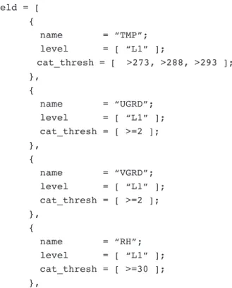
field = [ {

name = “TMP”; level = [ “L1” ];

cat_thresh = [ >273, >288, >293 ]; },

{

name = “UGRD”; level = [ “L1” ]; cat_thresh = [ >=2 ]; },

{

name = “VGRD”; level = [ “L1” ]; cat_thresh = [ >=2 ]; },

{

name = “RH”; level = [ “L1” ]; cat_thresh = [ >=30 ]; },

for chemical compounds and particles, O

3

, NO, NO

2

,

CO, SO

2

, PMTC and PMTF :

{

name = “OZCON”; level = [ “L1” ];

cat_thresh = [ >=50, >=110 ]; GRIB1_ptv = 129;

}, {

name = “NO”; level = [ “L1” ];

Table I. Chemical species description and grib table version and code

Version

Code Parameter

Units

Abbrev

129

156 Particulate matter (coarse)

mg m

–3

_PMTC

129

157 Particulate matter (fine)

mg m

–3

_PMTF

129

180 Ozone concentration

µl m

–3

_OZCON

141

141 Nitrogen oxide

µl m

–3

_NO

141

142 Nitrogen dioxide

µl m

–3

_NO

2

141

148 Carbon monoxide

µl m

–3

_CO

141

166 Formaldehyde

µl m

–3

_FORM

141

232 Sulfur dioxide

µl m

–3

_SO

2

(4)

}, {

name = “NO2”; level = [ “L1” ];

}, {

name = “CO”; level = [ “L1” ];

}, {

name = “SO2”; level = [ “L1” ];

}, {

name =”PMTF”; level = [ “L1” ];

}, {

name =”PMTC”; level = [ “L1” ];

cat_thresh = [ >=65, >=130 ];

GRIB1_ptv = 129; }

];

For a demonstrative purpose, gas pollutants

cate-gorical threshold values were set on the 1-h average

air quality standard (upper value) and half of the

standard (lower value).

4. Results

A high weekend ozone episode was considered to

show a comparison between model and observed data

by using MET and UPP modified codes. The episode

took place in Mexico City from 06:00 LT on April

13, 2007 through 03:00 LT on Apr 15, 2007. During

that period, measurements of criteria pollutants were

made by RAMA. Although it is possible to extract

the model formaldehyde concentrations during this

episode, this compound was not measured.

WRF-chem was configured to use the chemical

mechanism RADM2 as the chemical module

(Stock-well

et al

., 1990). The emissions inventory was

grid-ded based on the National Emission Inventory for the

Mexico City Metropolitan Area (MCMA) for the year

2006 (SMA, 2015). These emissions were updated

to fill in a 3-km spatial resolution and simulations

were carried out for a 40-h time period. Finally, the

observational data, required by MET, is provided by

the MCMA monitoring stations (RAMA). Figures 1

and 2 show examples where simulations are

com-pared against monitoring stations data.

0 1000 2000

12:00 00:00 12:00

0 20 40 60 80 100

O3 RAMA

Apr 13 15:00 h O3 ppbV

Apr 14 15:00 h

12:00 00:00 12:00

3000

O3 concentration in Cerro de la Estrella (CES) monitoring station CO concentrations in San Agustin (SAG) monitoring station

O3 WRF-Chem

CORAMA

Apr1315:00h COppm

Apr1415:00h O3 WRF-Chem

(5)

The Point-Stat tool computes several statistics

to evaluate the forecast performance in monitoring

stations. Figure 1 shows the simulated and observed

concentrations of O

3

and CO in ground-base stations.

To the left, the ozone concentration in the Cerro

de la Estrella (CES) monitoring station is shown.

The simulations (continuous line with fill squares)

fit well with the observation data (filled circles) in

most of the time domains, except for the high ozone

concentration time interval, where the simulations

underestimate the ozone peak (Apr 14, 15:00 LT).

Conversely, illustrated on the right side of Figure 1,

the simulated CO concentrations at San Agustín

(SAG) monitoring station are well fitted in the high

measured ozone concentrations. The CO simulated

concentrations systematically underestimate the

measurements, but almost follow the same observed

data pattern, which could indicate that the emission

inventory should be modified in that case. Also it

is possible that MET computes the grid average of

fields; the Stat-Analysis tool provides verification

statistics for a matched forecast and observation grid.

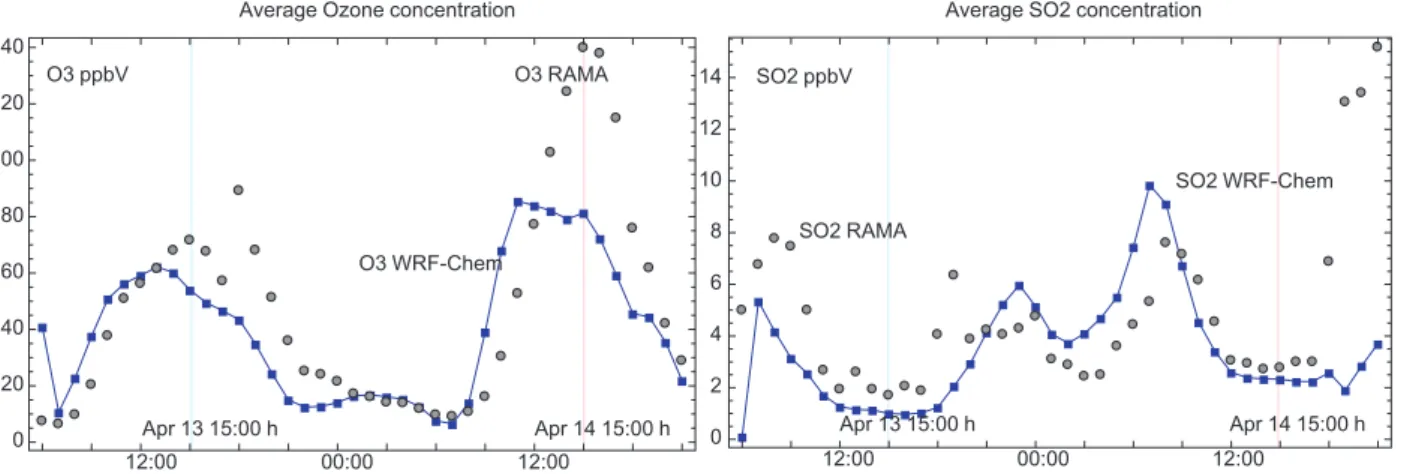
Figure 2 shows the point averages of the

observa-tions and simulaobserva-tions, the simulated variables

(con-tinuous line with fill squares) are compared against

the average of all RAMA stations (filled circle). On

the left in figure 2, the average ozone concentration

against RAMA data is shown. The maximum ozone

concentration occurred at 15:00h Apr 14 (Saturday)

and is pretty close to 140 μL m

-3

_{(ppbv), this value}

is bigger than the previous day maximum Apr 13

(Ozone weekend effect). The ozone numerical

simu-lation concentrations underestimate the second ozone

peak; the model concentration value is approximately

42% of the measured value. This pattern is presented

in other monitoring stations indicating that the model

underestimates the ozone concentration. In figure 2

(right panel) the average SO

2

concentration for model

and observations is shown. This chemical species is

well reproduced by the model especially in the first

hours of the high concentration episode.

Ambient concentrations depend on the emissions

and weather conditions. In the studied episode,

primary pollutants (CO and SO

2

) concentrations

have a better agreement with the measurements than

secondary pollutants (O

3

). The O

3

concentration

depends on primary pollutants like NO

2

and

Vol-atile Organic Compounds (VOC), and the highest

ambient concentration is reached downwind from

its precursor emissions. Because CO and SO

2

con-centrations from the model are in agreement with

measurements, and they are primary pollutants that

depend on local emissions, the high O

3

concentra-tions on April 14 suggest that this pollutant was

transported from elsewhere.

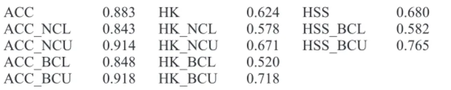
Additionally, Table II shows examples of several

verification measurements for SO

2,

including the

normal and bootstrap lower and upper confidence

limits (NCL, BCL, NCU and BCU). In this case the

threshold concentration were 130 ppb in order to

compute the categorical statistics. The first

param-eter shown on this table correspond to the accuracy

Fig. 2. Simulated and observed averaged fields, from April 13, 2007 at 6:00 LT to April 14 at 03:00 LT, in Mexico

City. Continuous line represents the average field calculated with the WRF-chem model, and filled circles represent

the average measured field from RAMA in the MCMA.

Average Ozone concentration Average SO2 concentration

12:00 00:00 12:00

0 20 40 60 80 100 120 140

O3 RAMA

Apr 13 15:00 h O3 ppbV

Apr 14 15:00 h O3 WRF-Chem

0 2 4 6 8 10 12 14

12:00 00:00 12:00

SO2 RAMA

Apr 13 15:00 h SO2 ppbV

(6)

Table II. Statistical analysis results for SO

2

evaluation. Accuracy (ACC),

Hansen-Kuipers Discriminant (HK) and Heidke Skill Score (HSS) for 662

total observations.

ACC

0.883 HK

0.624 HSS

0.680 ACC_NCL

0.843 HK_NCL

0.578 HSS_BCL

0.582 ACC_NCU

0.914 HK_NCU

0.671 HSS_BCU

0.765 ACC_BCL

0.848 HK_BCL

0.520 ACC_BCU

0.918 HK_BCU

0.718 (ACC) contingency parameter. In our simulation

ACC = 0.883, meaning the fraction of forecast that

was correct, ACC ranges from 0 to 1, perfect forecast

has an ACC value of 1.

The two other parameters are the

Hanssen-Kui-pers Discriminant (HK) and the Heidke Skill. Its

values range from –1 to 1. A perfect forecast has

HK = 1, and a value of 0 indicates no skill. HSS is

a skill score based on accuracy with values ranging

from −∞ to 1. A perfect forecast will have an HSS

= 1. For a more comprehensive description of these

and other verification measurements, see Appendix C,

Verification measures on the MET Users Guide v5.2.

5. Conclusions

The modifications made in the UPP code can provide

files that include pollutant concentration variables

(i.e., O

3

, CO, SO

2

, PM

10

and PM

2.5

, among others);

these files can be used by MET in order to evaluate

objectively the model performance with a set of

statistical parameters. A demonstration of the

func-tionality of the code modifications was presented

through its application in the case study, which

showed that CO and SO

2

model concentrations

have a better agreement than O

3

when compared

to measured values. In the case of O

3

, the first day

presents a good agreement, but for the second day

its concentrations could indicate that it comes from

elsewhere.

These code additions can reduce the time for data

analysis and standardize the evaluation procedure

for chemical and meteorological variables by using

a state-of-the-art suite of verification tools.

Acknowledgment

The authors want to tanks Paul Oldenburg and

John Halley Gotway from Meted-UCAR for their

support.

References

Baldwin M., H.-Y. Chuang, L. Bernardet, D. Jovic, R.

Rozumalski, W. Ebisuzaki and L. Nance, 2012. User‘s

cuide for the NMM core of the Weather Research and

Forecast (WRF) modeling system version 3. Chapter

7. Post Processing Utilities. NCAR/MMM, 2012.

COLA, 2015. Grid Analysis and Display System (GrADS).

Available at: http://www.iges.org/grads/.

DTC, 2015. Developmental Testbed Center. Available at:

http://www.dtcenter.org (last accessed on June 10, 2017).

Fast J.D., W.I. Gustafson, R.C. Easter, R.A. Zaveri, J.C.

Barnard, E.G. Chapman, G.A. Grell and S.E. Peckham,

2006. Evolution of ozone, particulates, and aerosol

direct radiative forcing in the vicinity of Houston using

a fully coupled meteorology-chemistry-aerosol model.

J. Geophys. Res.-Atmos. 111.

DOI: 10.1029/2005JD006721

Gotway J. H., R. Bullock, P. Oldenburg, T. Jensen, L.

Holland, B. Brown, T. Fowler, D. Ahijevych and E.

Gilleland, 2014. Model Evaluation Tools Version 3.0.1

(METv3.0.1). Development Testbed Center, Boulder,

Colorado.

Grell G.A., S.E. Peckham, R. Schmitz, S.A. McKeen,

G. Frost, W.C. Skamarock and B Eder, 2005. Fully

coupled “online” chemistry within the WRF model.

Atmos. Environ. 39, 6957-6975.

NCAR, 2015. The NCAR Command Language (NCL).

Available at: http://www.ncl.ucar.edu/overview.shtml.

ON388, 2013. Parameters and UNITS Table 2. Available

at: http://www.nco.ncep.noaa.gov/pmb/docs/on388/

table2.html.

SMA, 2015. Inventario de Emisiones de Contaminantes

de la Zona Metropolitana del Valle de Mexico 2008.

Secretaría de Medio Ambiente, Mexico City. Available

at: http://www.aire.df.gob.mx/.

(7)

PM

10

, and O

3

during 1986-2007. Atmos. Chem. Phys.

Discuss. 8, 8357-8384. doi: 10.5194/acp-8-5313-2008

Stockwell W.R., P. Middleton, J.S. Chang and X. Tang,

1990. The second-generation regional acid deposition

model chemical mechanism for regional air quality

modeling. J. Geophys. Res. 95, 343-16,367.

(8)

A1 VRBLS3D_mod.f

After line 27 ! Add GFS fields

,O3(:,:,:),O(:,:,:),O2(:,:,:)& ,NO(:,:,:),NO2(:,:,:),SO2(:,:,:),-CO(:,:,:) &

,HCHO(:,:,:),PMTC(:,:,:) ,PMTF(:,:,:)

A2 ALLOCATEALL.f

After line110 !GFS FIELD

allocate(o3(im,jsta_2l:jend_2u,lm)) ...

allocate(NO(im,jsta_2l:jend_2u,lm)) allocate(NO2(im,jsta_2l:jend_2u,lm)) allocate(SO2(im,jsta_2l:jend_2u,lm)) allocate(CO(im,jsta_2l:jend_2u,lm)) allocate(HCHO(im,jsta_2l:jend_2u,lm)) allocate(PMTC(im,jsta_2l:jend_2u,lm)) allocate(PMTF(im,jsta_2l:jend_2u,lm))

A3 RQSTFLD.f After line 1611

! GFS fields Chemistry Add

DATA IFILV(510),AVBL(510),IQ(510),I S(510),AVBLGRB2(510) &

& /1,’SO2 ON MDL SFCS ‘,232,109,&

& ‘SO2 con-centration ppb’/ !table 141 232 DATA IFILV(511),AVBL(511),IQ(511),I S(511),AVBLGRB2(511) &

& /1,’CO ON MDL SFCS ‘,148,109,&

& ‘CO concen-tration ppb’/ !table 141 148 DATA IFILV(512),AVBL(512),IQ(512),I S(512),AVBLGRB2(512) &

& /1,’HCHO ON MDL SFCS ‘,166,109,&

& ‘Formal-dehyde conc ppb’/ !table 141 166 DATA IFILV(513),AVBL(513),IQ(513),I S(513),AVBLGRB2(513) &

& /1,’O3 ON MDL

Appendix A. Specific modifications for UPP files

SFCS ‘,180,109,&

& ‘Ozone conc. ppb ‘/ !table 129 180

& /1,’SURFACE O3 CONC ‘,180,100,&

& ‘Ozone surf conc ppb ‘/ !table 129

DATA IFILV(515),AVBL(515),IQ(515),IS (515),AVBLGRB2(515) &

& /1,’PMTC ON MDL SFCS ‘,156,109,&

& ‘PM 10 conc ug/m3 ‘/ !table 129 156

DATA IFILV(516),AVBL(516),IQ(516),IS (516),AVBLGRB2(516) &

& /1,’PMTF ON MDL SFCS ‘,157,109, &

& ‘PM 2.5 conc ug/m3 ‘/ !table 129 157

& /1,’NO ON MDL SFCS ‘,141,109,&

& ‘NO concen-tration ppb ‘ / !table 141 141 DATA IFILV(518),AVBL(518),IQ(518),I S(518),AVBLGRB2(518) &

& /1,’NO2 ON MDL SFCS ‘,142,109,&

& ‘NO2 con-centration ppb’ / !table 141 142

A4 DEALLOCATE.f

Include the following lines after line 111: !GFS FIELD

(9)

A5 INITPOST.F

After line 48.

use vrbls3d, only: t, u, uh, v, vh, wh, q, pmid, t, omga, pint, alpint,&

qqr, qqs, qqi, qqg, qqni,qqnr, cwm, qqw, qqi, qqr, qqs, extcof55,&

f_ice, f_rain, f_rimef, q2, zint, zmid, cfr, REF_10CM, &

o3,co,no,no2,so2,pmtf,pmtc,hcho After line 341. (Because WRF-chem model has gas concentrations in ppm a conversion to ppb is made multiplying by 1000 only gas chemical variables).

print*,’finish reading mixing ratio’ ! For Particulate Matter (Coarse) PM10 VarName=’PM10’

call getVariable(fileName,DateStr,-DataHandle,VarName,DUM3D, &

IM+1,1,JM+1,LM+1,IM,JS,JE,LM) do l = 1, lm

do j = jsta_2l, jend_2u do i = 1, im

PMTC( i, j, l ) = dum3d ( i, j, l )

end do

end do end do

! For Particulate Matter (Fine) PM2.5 VarName=’PM2_5_DRY’

call getVariable(fileName,DateStr,-DataHandle,VarName,DUM3D, &

PMTF( i, j, l ) = dum3d ( i, j, l )

end do end do end do

print*,’finish reading PM10 and PM2.5 concentrations’

! For Ozone O3 VarName=’o3’

call getVariable(fileName,DateStr,Da-taHandle,VarName,DUM3D, &

O3( i, j, l ) = dum3d ( i, j, l )*1000.

! For Nitrogen Oxides NO VarName=’no’

NO( i, j, l ) = dum3d ( i, j, l )*1000.

! For Nitrogen Dioxide NO2 VarName=’no2’

NO2( i, j, l ) = dum3d ( i, j, l )*1000.

! For Sulfur Dioxide SO2 VarName=’so2’

SO2( i, j, l ) = dum3d ( i, j, l )*1000.

(10)

CO( i, j, l ) = dum3d ( i, j, l )*1000.

! For Formaldehyde HCHO VarName=’hcho’

HCHO( i, j, l ) = dum3d ( i, j, l )*1000.

print*,’*** Finish reading gas chem-ical concentrations’

A6 MDLFLD.f

After line 82

use vrbls3d, only: zmid, t, pmid, q, cwm, f_ice, f_rain, f_rimef, qqw, qqi,& qqr, qqs, cfr, dbz, dbzr, dbzi, dbzc, qqw, nlice, nrain, qqg, zint, qqni,& qqnr, uh, vh, mcvg, omga, wh, q2, ttnd, rswtt, rlwtt, train, tcucn,& o3, rhomid, dpres, el_pbl, pint, icing_gfip, icing_gfis, REF_10CM,& co,no,no2,so2,pmtf,pmtc,hcho

After line 2049

! Nitrogen Oxide (NO) ON MDL SURFACES. IF (IGET(517).GT.0) THEN

IF (LVLS(L,IGET(517)).GT.0) THEN LL=LM-L+1

ID(1:25) = 0 ID(2)=141

!$omp parallel do private(i,j) DO J=JSTA,JEND

DO I=1,IM

GRID1(I,J)=NO(I,J,LL) ENDDO

ENDDO

if(grib==”grib1”) then CALL GRIBIT(IGET(517),L,GRID1,IM,-JM)

else if(grib==”grib2” )then cfld=cfld+1

fld_info(cfld)%i-fld=IAVBLFLD(IGET(517))

fld_info(cfld)%lvl=LVLSXM-L(L,IGET(517))

!$omp parallel do private(i,j,jj) do j=1,jend-jsta+1 jj = jsta+j-1 do i=1,im

datapd(i,j,cfld) = GRID1(i,jj)

enddo enddo endif ENDIF

ENDIF

! Nitrogen Dioxide (NO2) ON MDL SURFACES. IF (IGET(518).GT.0) THEN

ID(1:25) = 0 ID(2)=141

!$omp parallel do private(i,j) DO J=JSTA,JEND DO I=1,IM

GRID1(I,J)=NO2(I,J,LL) ENDDO

ENDDO

(11)

do i=1,im

ENDIF

! Sulfur Dioxide (SO2) ON MDL SURFACES.

IF (IGET(510).GT.0) THEN

ID(1:25) = 0 ID(2)=141

GRID1(I,J)=SO2(I,J,LL) ENDDO

ENDDO

ENDIF

! Carbon Monoxide (CO) ON MDL SURFACES.

ID(1:25) = 0 ID(2)=141

GRID1(I,J)=CO(I,J,LL) ENDDO

ENDDO

ENDIF

! Formaldehyde (HCHO) ON MDL SUR-FACES.

ID(1:25) = 0 ID(2)=141

GRID1(I,J)=HCHO(I,J,LL) ENDDO

ENDDO

(12)

ENDIF

! OZONE (O3) ON MDL SURFACES. IF (IGET(513).GT.0) THEN

ID(1:25) = 0 ID(2)=129

GRID1(I,J)=O3(I,J,LL) ENDDO

ENDDO

ENDIF

! PMTC (PM10) ON MDL SURFACES. IF (IGET(515).GT.0) THEN

ID(1:25) = 0

ID(2)=129

GRID1(I,J)= PMTC(I,J,LL) ENDDO

ENDDO

ENDIF

! PMTF (PM2.5) ON MDL SURFACES. IF (IGET(516).GT.0) THEN

ID(1:25) = 0 ID(2)=129

GRID1(I,J)= PMTF(I,J,LL) ENDDO

ENDDO

(13)

ENDIF !

! ---- ADD GOCART FIELDS

A7 wrf cntrl.parm

Additional lines to be add.

(O3 ON MDL SFCS ) SCAL=( 4.0)