comment
reviews
reports
deposited research
interactions
information
refereed research
Research
Model-based cluster analysis of microarray gene-expression data
Wei Pan*, Jizhen Lin
†
and Chap T Le*
Addresses: *Division of Biostatistics, School of Public Health, University of Minnesota, 420 Delaware Street SE, Minneapolis, MN 55455-0378, USA. †Department of Otolaryngology, School of Medicine, University of Minnesota, 2001 6th Street SE, Minneapolis, MN 55455, USA. Correspondence: Wei Pan. E-mail: [email protected]
Abstract
Background:Microarray technologies are emerging as a promising tool for genomic studies. The
challenge now is how to analyze the resulting large amounts of data. Clustering techniques have been widely applied in analyzing microarray gene-expression data. However, normal mixture model-based cluster analysis has not been widely used for such data, although it has a solid probabilistic foundation. Here, we introduce and illustrate its use in detecting differentially expressed genes. In particular, we do not cluster gene-expression patterns but a summary statistic, the t-statistic.
Results: The method is applied to a data set containing expression levels of 1,176 genes of rats
with and without pneumococcal middle-ear infection. Three clusters were found, two of which contain more than 95% genes with almost no altered gene-expression levels, whereas the third one has 30 genes with more or less differential gene-expression levels.
Conclusions:Our results indicate that model-based clustering of t-statistics (and possibly other
summary statistics) can be a useful statistical tool to exploit differential gene expression for microarray data.
Published: 29 January 2002
GenomeBiology2002, 3(2):research0009.1–0009.8
The electronic version of this article is the complete one and can be found online at http://genomebiology.com/2002/3/2/research/0009 © 2002 Pan et al., licensee BioMed Central Ltd
(Print ISSN 1465-6906; Online ISSN 1465-6914)
Received: 26 September 2001 Revised: 7 November 2001 Accepted: 28 November 2001
Background
The pattern of genes expressed in a cell can provide impor-tant information about the cell state. DNA microarray tech-nology can measure the expression of thousands of genes in a biological sample. DNA microarrays have been increas-ingly used in the last few years and have the potential to help advance our biological knowledge at a genomic scale [1,2]. In analyzing DNA microarray gene-expression data, a major role has been played by various cluster-analysis techniques, most notably by hierarchical clustering [3], K-means cluster-ing [4] and self-organizcluster-ing maps [5]. These clustercluster-ing tech-niques contribute significantly to our understanding of the underlying biological phenomena. A recent review of various methods is provided by Tibshirani et al. [6]. However, many methods, including the three mentioned above, have some
restrictions, one of which is their inability to determine the number of clusters. The difficulty may be related to the fact that in many methods there is no clear definition of what a cluster is in the first place. Furthermore, their clustering results may not be stable [7,8]. An important clustering technique that improves on and/or provides alternative solutions to these issues is model-based clustering (see, for example, [9]). It has a clear definition that a cluster is a sub-population with a certain distribution, and several statistical methods can be applied to estimate the number of clusters. Some authors have considered its application to cluster gene-expression patterns [10-12].
to identify all the genes with altered expression under two experimental conditions (for example, normal cells versus cancer cells). We note that the goal here is different from that of clustering gene-expression patterns, as done by other researchers in using model-based clustering. In modeling differential expression levels of genes, it is natural to assume that genes are from two subpopulations, one with constant and another with changed expression levels. Hence, a two-component mixture is a reasonable model. This is the approach proposed by Lee et al.[13], where it is assumed that each of the two components has a normal (in the statis-tical sense) distribution. However, in general, each compo-nent does not necessarily have a normal distribution. It is well known that many distributions can be well approxi-mated by a finite mixture of normal distributions. Hence, the normal mixture model-based clustering can be regarded as a more general and flexible approach along these lines and we pursue this approach here. In particular, we summarize a possible change of expression of a gene using a t-statistic, which automatically accounts for differential variations of expression levels across genes. Then we apply model-based clustering to these t-statistics to exploit which genes have differential expression levels. The methodology is illustrated with an application to a dataset containing the expression levels of 1,176 genes of normal rats and those with pneumo-coccal middle-ear infection.
Results and discussion
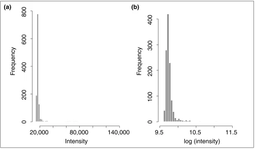
Data and preprocessingPneumococcal otitis media is one of the most common dis-eases in children. Almost every child in the United States experiences at least one episode of acute otitis media by the age of 5 years. To understand the pathogenesis of otitis media, it is important to identify genes involved in response to pneumococcal middle-ear infection and to study their roles in otitis media. A study was recently carried out at the University of Minnesota, applying radioactively labeled cDNA microarrays [14] to the mRNA analysis of 1,176 genes in middle-ear mucosa of rats with and without subacute pneumococcal middle-ear infection. It consisted of six experiments: two cDNA microarrays were run with controls while four were run with pneumococcal middle-ear infec-tion. We first take a natural logarithm transformation for all the observed gene-expression levels so that they are more likely to have a normal distribution, which will reduce the number of clusters found in a model-based clustering. The histograms of gene-expression levels before and after log-transformation for the first experiment are shown in Figure 1. It can be seen that the log-transformation reduces the skewness of the distribution of gene-expression levels.
[image:2.609.56.558.414.710.2]After taking log-transformation, for each experiment we then standardize the transformed gene-expression levels by
Figure 1
Histograms of radioactivity intensity levels for the first experiment, a cDNA microarray analysis of 1,176 genes in middle-ear mucosa of healthy (control) rats. (a)Before log-transformation; (b)after log-transformation.
20,000
80,000
140,000
0
200
400
600
F
requency
F
requency
800
Intensity
9.5
10.5
11.5
0
100
200
300
400
log (intensity)
comment
reviews
reports
deposited research
interactions
information
refereed research
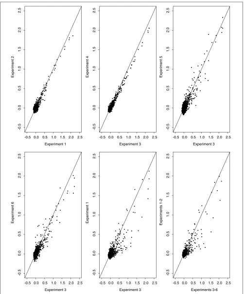
subtracting their median value. The above standardization is based on the assumption that most genes, at least a half, will not be expressed. The median is used because it is more robust against outliers than is the more commonly used mean. We use xijto denote the resulting expression level of gene ifrom experiment j. Note that the first two experiments (that is, j= 1 and 2) were conducted using control rats whereas the last four (that is, j= 3, 4, 5, 6) using infected rats. Some scatterplots showing comparisons between experiments are presented in Figure 2. It can be seen that, in general, there is a good agreement as well as some variation between the experiments under the same condition, that is, either within the control group or within the infected group. It appears that expression of some genes are altered with pneumococcal infection.
On the basis of the above observation, we calculate the fol-lowing two-sample t-statistic for each gene as its measure of possible differential expression:
zi1- zi0
yi= —————————————————————————— ,
冱
j=3冢xij - zi1冣2
冱
j=1 冢xij - zi0冣2
————————————+ ———————————
4(4-1) 2 (2-1)
where:
6 2
zi1=
冱
xij/4,zi0=冱
xij/2j=3 j=1
for i = 1, ... ,1176. The numerator of yiis the difference of average gene-expression levels under the two conditions (infected versus control), whereas the denominator is the sample standard error of the numerator and serves to stan-dardize the observed difference by penalizing those with large (and thus less reliable) variations. Previous studies have found evidence that genes may have differential vari-ability of expression levels [15-17]. Note that although the
t-statistic is constructed, we shall not conduct t-tests because there is no evidence to support the questionable normality assumption required by the t-test. We also do not carry out permutation or other nonparametric tests [18] because of the small sample size (that is, 2 + 4). This is also related with the fact that there exists the problem of multiple compar-isons if we test gene by gene [18]. Our goal here is to apply model-based cluster analysis to the preprocessed relative gene-expression levels yi, i= 1, ... , 1176, and see which genes will have relative levels far away from the majority.
Model-based clustering
Finite mixtures of distributions provide a flexible as well as rigorous approach to modeling various random phenomena (for example, [19]). For continuous data, such as gene-expression data, the use of normal components in the
mixture distribution is natural. With a normal mixture model-based approach to clustering, it is assumed that the data to be clustered are from several subpopulations (or clusters or components) with distinguished normal distribu-tions. That is, each data point yis taken to be a realization from a normal mixture distribution with the probability density function:
g
f(y; g) =
冱
5i1(y; 2i,Vi), (1)i=1
where 1(y; 2i, Vi) denotes the normal density function with mean 2iand (co)variance matrix Vi, and 5i’s are mixing pro-portions. We use g to represent all unknown parameters (5i, 2i, Vi): i= 1, ... gin a g-component (or g-cluster) mixture
model.
In model-based clustering, first, the above mixture model is fitted to the data and obtain the maximum likelihood esti-mate ^g. Second, the posterior probabilities of each data point belonging to each of the gnormal components can be calculated. Finally, each data point is assigned to the compo-nent with the largest posterior probability. We review the major steps in the following.
The mixture model is typically fitted by maximum likelihood using the expectation-maximization (EM) algorithm [20]. Given nobservations y1, ..., yn, we want to maximize the log-likelihood
n
log L(g) =
冱
log f(yj; g)j=1
to obtain the maximum likelihood estimate ^g. The EM algo-rithm computes ^gby iterating the following steps.
Suppose that at the kth iteration, the parameter estimates are 5i(k)’s, 2i(k)’s and Vi(k)’s. Then in the (k+ 1)th iteration, the
estimates are updated by
n
5i(k+1) =
冱
9ij(k)/n, j=1n n
2i(k+1) =
冱
9ij(k)yj/冱
9ij(k), j=1 j=1冱nj=19ij(k)冢yj - 2i(k+1)冣冢yj - 2i(k+1)冣T Vi(k+1) = ——————————————————————— ,
冱nj=19ij(k)
Figure 2
Comparison of the log-transformed, standardized expression data between experiments. Experiments 1 and 2 were conducted using control rats; experiments 3-6 used infected rats.
•••••• •• • • • ••• •• • •• • • • •••••••••• • • • • ••• • ••• • ••• • •• • •• •• • • • •••••• •• • • • • • •• • • • • •• • • • • • • • • • • • •• • ••• • • • ••• •• • •• • • • •• ••• • • • • • • • •••• •••••• • ••• • • • • •• •• ••••••• • • • • • ••• • ••••• •• • ••••• ••• • • • •• • • • • •• • •• • • ••••• •• • • •• ••••••••• •••• • • •• ••• • • • • • • • • •• • •• • • • • • •••• • ••••• • •• • • ••••• • •• ••••• • ••••• • • • ••• • •• • • • • • •• • •• • • • • •• • •••• • ••• ••• • ••• • • ••••• •• •• • • • •••• • ••• ••• • • • • ••• •• ••• ••• • • • •••• ••• ••• • ••• ••••• •••• • • •• • • ••• • ••• • • • • •• • • • • • • • • • •• •••• • • • • • • • • • ••• • • • • • • ••• • •• • •• • • • • • •• • • •• •• • • • • • • • • • • • • ••• • • • • •• • • • ••• •• • • • • • • • • • • •• • • • • • • •• • • • • • ••• • • • • • •• • • •••• • • • • • • •• • • • •• • •• • •• • • • • • • •• •• • • • • • • • • •• • ••• • • • • •• • • • • • •• • • • • • • •••• • • • • • • • • • •• •••••••••••• • •• • •••• • • • •• • •••••••• • •• • •• • • • • ••• • •• • • • • •••••• • • • • • • • ••• • ••••••••••• ••• •••••• • • • •••• •••• • ••• ••••• • •••••••• ••••• • •••• • • • •••• • • • • •• • ••• •• ••• •• •• ••• •••••••••••••••• •• •• •• ••• • • •• • ••• •••••• • • • •••••• • •• • • ••••• ••• ••• • • • • • • •• •••• • • • • • • •••• •••• ••••• ••••• •• •• •• • •• • • • •• •••••• ••••••• • •• •• • • •••• • • • • •••• • • •• • •••• • •••••• • • • • • • ••• •••••• •• • • • •••• ••• • • ••• • ••••••••••• • • ••••••••••• • • •• • ••• • • • ••• •• • •• • •••••••• • •• • • • •• • ••• ••• • •• •• • • • • • • •••••• ••••• • ••• ••• • • •• • • ••• • ••• •• •••• • • ••••••• ••••••••••• •• • •• • • •••••••• • • •• •• ••• • •• ••••• • • • • • • • ••• ••• •• • ••• • • • •• • • • ••• • ••• • ••• • • •• • •••••• • • • Experiment 1 Exper iment 2
-0.5 0.0 0.5 1.0 1.5 2.0 2.5
-0.5 0.0 0 .5 1.0 1 .5 2.0 2 .5 • • • • • • • •• •• • • •••••• • •• •••• • • ••• •• • • • •• • • •• •• •• • • • • •• • • • • • ••• •• • • • • • • • • • ••• • • • • • • • • • •• • • • • • • • • •••• • • •• • • • • • • ••••••• •• • • • •• •• • • • •• • • • •• •••• • • • •••••• • • ••• • • • •• • • •• • •• • • •• • • •• • ••• • • • •• • • • ••• • • • • • • • • • • • •••••••••• •• • • •• •• •• • •••• • • •••••• • ••••• • • • ••• ••••• • • •• • • • • •••• • • •••• • •• • • • • • • • •• • • ••••• • • •• ••• • •• • •• ••••• • •• •• • • • ••• • • •• • • • • • ••• • • • • • • • • • •••••• • • ••• •• • •• •••• •• • • • • • • •• • • ••••• •••• ••••• • ••• • • • •• • •• • • • • • • ••• • • • •• •• • • •• • •• • •• • • • •• •• •• • •• • • • • • • • •• •• • •• • • • •• • • • • • • • • • • • • • • • • • •••••• • • • • • • • • ••••• • • • • • • • • • •• • • • • • • ••• • • • • •• • • • • • • • • • • •• • • •• • • • • ••• • • •••• • •• • • • •• • • • •••• • • • • • • • • • •• • • • • • • •• • • • ••••• • • • • •••• ••• • • • • • • •• • • •••••• •••• • • • • •• ••••••• • • • • • ••••• • • ••••• •• ••••• • • •••••••••• • •• • • •• • •• •• • ••••••••••••• •••• • • • •• • • • ••• •••• • •• •••• • • •• • • • • •• • ••••••• • • • ••• • •• • •••• • • • • •• • • • • • • • ••••• •• • • • • • ••••••• • • • • •• • •• • •• • • • • ••• • • •• • • •• • • • • • • • • • •••• • • •• •• • • • • ••• • • ••• • • • • • • • • • • • • •• • • • •• • • •••• •• • • • • ••••• • •• • • • • • • • • • • • • • • • ••• ••••• • •• ••••• • • • • • • • • • • •• •• • ••• •• • •• • • ••••••••••• • • • • ••• • • • • • • • • • • ••••• • • • •••• ••••• • •• • • • • •• • •••• • • • •••• • •• • • •• • • •• • • ••••••• • •• •• ••••• ••• • • • • • • • • • • • •••• • • •• • • • •• • •••• ••• • • •••••••• • • • •• •••• • ••• • •• • ••••••••••••••••••••• • ••• • •• • •• •• •• • •• • • • • • • •• •••• • • • • • • • •• • ••• • • • •• • • • • • ••• •• • •• • • • • • • Experiment 3 Exper iment 4
-0.5 0.0 0.5 1.0 1.5 2.0 2.5
-0.5 0.0 0 .5 1.0 1 .5 2.0 2 .5 • • • • • • ••• • • •• •••••• • •• •••• • • ••• • • • • • ••• • •• ••• • • •• • •• • • • • • • •• ••• • •• • • • • • ••• • • • • • • • • • • • •• • • • • • • • ••• • ••• • • • • • ••••• • • •• • • • • •• •• • • • ••• • • • • •• •• • • • • ••• • •• • • • • • • • ••• • •• • •• • • •• • • •• • •••• • • •• • • • • •• •• • • • •••• • • • •• •• •••• • •• • • •• •• • • • • ••• • • • • •• •• ••••• • • • • • •• ••••• • • •• • • • • •••• • •••• • • ••••••• • • •• • • • • • •• • • ••••• • • • • • • •• •••••••••••••• • • • • •• • •• • • •• • • • • • •• •• •••• •• • ••• •• • • • •• • • • •• • • • • • •• • • •• • ••• ••• • • ••• •••• • • • • • • • • • • • • • • ••• • • • • • •• • • •• • • • • • • • • • •• ••••• •• • • • ••• • • • •• • • • • • • • • • • • • • • • • • • • • •• • • • • • •••• • • • • • • • • • •••• • • • • • • • • • •• • • • • • • ••• • • • • • • • • • • • •••• • • • • • • • • • • • • •• • • • • ••• • • • • • • • • •• •••• • • • • • • • • •• •• • • • • • • • • • • • • • • • • • • • • ••• ••• • • • • • • • • • • ••• • •••• • • • • • • • • ••••• • • • •• • ••••• • • •• • • • •• •••• • • • • ••••••••• • •• • • • • ••• •• • •• • •• • • •• • • • • ••• • • •• •• • • •••••• • • • •• ••• • ••••••••• • • • • • • •• • • • • • • • • • • • •• •• • •• ••••• • • • • • •••• •• • • • • •• ••••• •• •• • • •• • •• • •• • • • • •• • • • •• • • • • •• • • • • • • • • •• •• •••• • • • • •••• • • • • •• • • • • • • • •• • • •• • • • • • • • • ••• •• • • • • • • ••• • • • • • • • • • • •• • •• • • • •••• • • • • • •• •••••• • • • • • • •• • •• •• ••• • • • • •••• •• •• ••• • •• • • • •• ••• • • • • • • • • • • • •••• ••••• • • •• • •• • •• • • • • • • • • ••• • • • •• • • • • • •• ••• • • • • • • •• • • •• • • • •••• • •• ••• • • •• • • • • • • • ••••• • ••• • • •• • ••• • •• •• • •• •••• • • • •• •• • • •• • •• • • • • • •••••••• •• • ••• • • • •• •• • •• • • •• ••• ••• • • • • • • • • • • • • ••• •• • • • • • • •• • ••• • • • •• •• ••• ••• •• • •• • • • • • • Experiment 3 Exper iment 5
-0.5 0.0 0.5 1.0 1.5 2.0 2.5
-0.5 0.0 0 .5 1.0 1 .5 2.0 2 .5 • • • • • • ••• •• ••• • • • • • • •• • •• • • • •• • • • • • • •• • • • • •• •• • •• • •• • • • • • ••• • •• • •• • • • • • •• • • • • • • • • • • • • • • • • • • • • • • •• • • • ••• • • • • ••••• • • •• • • • • • •• • • • •• • •• • • ••• • • • • ••••• ••• ••• • • • • • • • •• • ••• •• • • • •• • • •• • • • •• • • ••• • • • • • • • •••• • •••••••••• •• • •• • •• •• • • • •• • • •••••••• • • • • • • • ••• • • ••• • • • • • • • • •••• • • • • • ••••• •• • • • ••• • • •• • • • • • •• ••• • • • • •• •••••••• •••• •••••• •• • • • • • •• •• • • • • • • • • •• • • • • • • • • • •• • •• •• • ••••• • ••• ••• ••••••• • •• ••••• •••• • • • •• • ••• • • • • • • •• • • • •• •• • • •• ••• • • • • • • • • •••• • •• • • • • •• • •• • • •• • • • • •• • • • • •• • • • • • • • • • • • •••••• • • • • • • • • • ••• • • • • • • • • • • •• • • • • • • •• • • • • • • ••• • • • • • •• • • • • • •• • • • • • • •• • • • ••• • • • • • • • • • • • • • • • • • • • • • • • ••• • • • • • • • • • • •• • ••• • • • ••••••• • • •• • • • • • • •• •••• •••• • • •••• ••••••• • • •• • •••• • • • • • • • • • • ••••• • • • • •• •• •• •• • •• • • •• • •• • • ••••••••••• • • • •••• • • • •• ••• ••••• • • • •• •••• • • •••••• •• • •• • • • • • • • • ••• • • • • •• ••• ••••••• • • • • • ••••••• • • • •• • •••• •• • • • • •• • •• • •• • • • •••• • • • • • • •• • • • •••• • • ••••• ••• • • • • • • ••• • • •• •• • • • • • • • • • • • • • • • • •• • • • • •• •• • • • • • • • • • • •• • • • • • • • • • • ••• • • •••• •• • • • •• ••• • •• • • • • • • • • •• • •• •• • • • • • • •• • •• • •• •• •••• • • • • •••• • • • • • • • • • • •••••• • •••• •• ••• ••• • • • • • • • •••• • • • • •• • • •• •• ••• • •• • • • • • • • •• • • • •• • • •• •••••••• • • • • • • •• ••• • •• • •• • • • •••• ••• • • •• ••••• • • •••• •••• • ••• • •• • •••••• ••• • ••• • • • •• ••••••• •• ••• •• •• • •• • • • • • • •• ••• ••• ••• • ••• • •••• • • •• • • • • • •• • • • • •• • • • • • • Experiment 3 Exper iment 6
-0.5 0.0 0.5 1.0 1.5 2.0 2.5
-0.5 0.0 0 .5 1.0 1 .5 2.0 2 .5 • • •••• •• • •• •••• • •• • • •• ••• • • • •• • • • • • • ••• ••• • • •• ••••• •• • • • • • •• •••• •• • • • • • ••• • • • • • • • • • • • • • • • • • • • ••• • • ••••• • • • ••••• • • • • • • • • •••• • • • ••• • • • • •••• • • • •••• •••• •• • • • • • ••• ••• •••• • • • • •• • • •• • • • •• • • •••• •• • • • • • • • • • •••••• •••• • ••••• •• •••• • •• • • •• • • ••• ••••• • • • ••• ••• • • • • •• • • • • ••••• ••• • •• ••• • • • • • ••• • • •• • •• • • •• ••• • • • • • • •• •••••• •••• •••••• •• • •• •• • •• •• • ••• • • • ••••••••• • •• • •• • •• ••••• • • • • ••• • •••••••••• • • •• •••• • • • •• • • • •• • • ••• •• • • • •• •• • • •• • • • • • • • • • • • ••••• • • • • • • •• • • • •• •• • • • • • • • • • • • • • • • • • • • • • • • ••••• • • • • • • • • • ••••• • • • • • • • • • • • •• • • • • • •• • • • • •• • • • • • • ••• • • • •••• • • • • • • • • • ••••• •• • • • • • • • • •••• • • • • • • • • •• • • • • • • • • • • • • ••• ••• • • • • • • • •• • • • • • • • •• • • • • •• •• •••• • • • •• • ••••••••• ••• ••• • • • • ••••• •• ••••• • • • • •••••• •••• • • • •• ••• •• ••••• • •••••• • • •••• • •• ••• • •• •••• • • • •• •••• ••••• • •• •••••• •• • • • •• • • ••••• • ••• • •••••• • • • • •• ••••••• • • • • • •••••••••• • •• • •• • ••• • • • • •• •• • • • • • • •• • •• • •• • • •• •• • • • ••• • • •• •• •• • • •• • • • • • • •• • • • •••• ••••• • • •• •• •• • • •• ••• • • • • •• • • •• •• • •• •• • •••••• •••• • ••••• • • • • • • • •• • • • •• • • • • • • • •• • • •••••• • •••• • • •• • • ••• • • ••• • • • • •••••••••••••••••••• • • • •• • •••• • • • • • • • • • • • • ••• • • •• • ••••••• • •• • • •••••••• • • • • • • •• ••• •• •• • • ••• •• •• • •••• ••• • ••• •••••• • • • •• • ••• • ••• • •• • •••••• • • • • • ••• •• • • • •••• • • • •• ••• ••••••• • • • • •• • • ••• • •• •• •• ••• • ••••• • •• • •• • • ••• • • • •• • • • • • • Experiment 3 Exper iment 1
-0.5 0.0 0.5 1.0 1.5 2.0 2.5
-0.5 0.0 0 .5 1.0 1 .5 2.0 2 .5 • • •• •••• • •••••• • ••• • •• •••• • • •••• • • • • •••• •• •• ••••••• •• • • • ••••••• • •• • • • • • ••• • • • • •• • • • • • ••• • • • • • •••• • • ••• • • • • •••••• • • • • • • • • • ••••• •••••• • •••• • • • •• ••••••••• • • • ••• ••••••• • ••• • •• ••••• • • •• • • •• • ••••• • • •••• • ••••••••••• •• ••••• • • • •• •• • • • ••• • • •••• •• • • • •• • •••••••• • • • •• •••••••••••••• •• • • • ••• • • ••• • • • • ••••• • •• • ••••• •• •• • •••• •••• ••••••••••• ••• • • • • ••• • •••••••••• • • •• ••• •• ••• • ••• • • • ••••••••••••• •••••• •• • •• ••• ••• • • • • •• • • • • • • • • • •• • • •• • • • • • • • • •• •••• • • • ••• • •••• •• • • • • • •• • • • •• •• • • • • • • • • • ••••• • • • • • • • • • • •••• • • • • • • • • • • •• • • • • • • •• • • • ••• •• • • • • •• • • • • • ••• • • • • ••• • • •••••• • • • • • • • • • •••• • • • • • •• • • ••• • • • • • •• • • • • ••• • •• • • • •••••• • • ••• • • ••• ••••••••••• ••••• •••• • •• •••• •••••••• • •• ••• • ••••••• • •••• • •••• • •• ••• •• ••••••• • • ••••• •• •••• • • • ••• ••••••• • • • ••••• •• •••• • •• ••••• •• ••• • •• ••••••• • •••• ••••••• • • ••• ••••••••••••••• •••••••••••••• ••• • • • • ••• ••• • ••••• • •• • • •• • •••• • ••• • • • • • • •••••••• • • • • • • •• •••••••• •• ••• ••••••• • • • •••• • •••••••• • ••••• • • • ••••• • • • • •• ••••• • • • • • • • • •• •••••••• • • • • • • ••• •••••• •• • • • •• ••••• • • ••• • •• ••••••••••••••••• ••• • • • • • • • ••• • • • •• ••• • •• •• ••• • ••••• • ••••• • • • • ••••••••• • • • • • • ••••• ••••• • ••• •••• • ••• • ••• • ••••••••• • •••• •••• •••• • •• ••••••• • ••• ••••••••• •••••••• • ••• •• ••••• • • • • •• • ••• •••••• • • ••• • ••• •• • ••• • • •• •••••••• • • • • • • Experiments 3-6 Exper iments 1-2
-0.5 0.0 0.5 1.0 1.5 2.0 2.5
5i(k)1冢yj; 2i(k), Vi(k)冣
9ij(k) = ————————————————— , (2)
f冢yj; (k)冣
is the posterior probability that yjbelongs to the ith compo-nent of the mixture, using the current parameter estimate
(k)
g for g, for i= 1, ..., gand j= 1, ..., n.
At convergence, we obtain ^g= (B)
g as the maximum
likeli-hood estimate. As local maxima can be found by the EM algorithm, it is desirable to run the algorithm multiple times with various starting values and choose the estimate as the one resulting in the largest log-likelihood.
One interesting but difficult problem in cluster analysis is to determine the number of components g. In contrast to many other approaches that fail to accomplish this goal, model-based clustering provides several useful and objective selection crite-ria, which have been used in other model selection problems. The best known are the Akaike Information Criterion (AIC) [21] and the Bayesian Information Criterion (BIC) [22]:
AIC= -2 logL(^g) + 2vg,
BIC= -2 logL(^g) + vg log (n),
where 3gis the number of independent parameters in g. In
using the AIC or BIC, one first fits series of models with various values of g, then one picks up the gwith the smallest AIC or BIC.
In many studies related to model selection, it is found that AIC may select too large a model whereas BIC may select too small a model. This phenomenon appears to hold in selecting gin the mixture analysis [23]. Some other criteria have been studied but there does not seem to be a clear winner [23]. Banfield and Raftery [24] proposed using approximate weight of evidence as an approximate Bayesian model selection criterion. Some empirical studies seem to favor the use of BIC [25]. We feel that a combined use of AIC and BIC is helpful, at least in providing a range of reasonable values of g.
A different approach to selecting g is through hypothesis testing. This could be done through the use of the log-likeli-hood ratio test (LRT) to test for the null hypothesis H0: g=
g0against the alternative H1: g= g0+1 for any given positive integer g0. The LRT statistic is 2 log L(^g0+1) - 2 log L(^g0),
which, however, does not have the usual asymptotically chi-squared distribution as a result of violation of required regu-larity conditions (for example, the maximum likelihood estimate may lie in the boundary of its parameter space). McLachlan [26] proposed using the bootstrap to approxi-mate the distribution of the LRT statistic under the null hypothesis. On the basis of the resulting p value, one can decide whether to reject H0.
Implementation
McLachlan et al.[27] have implemented model-based clus-tering in a stand-alone Fortran program called EMMIX, which is freely available from the web [28]. It supports all the functions we described above, including multiple start of the EM algorithm using random partition or K-mean clus-tering, calculation of the model selection criteria AIC and BIC, and the use of the bootstrap to test a given number of components g0. We will use EMMIX to analyze the gene-expression data described earlier.
The MCLUST software [29], implementing model-based clustering, is also freely available [30]. It is designed to interface with the commercial statistical package S-Plus. For users familiar with S-Plus, it is convenient to take advantage of the power and flexibility of S-Plus. However, at the same time, it can have some serious restrictions on the size of the data being analyzed because of the overhead on CPU speed and memory induced by S-Plus.
Application
We fitted five mixture models with g ranging from 1 to 5. Table 1 summarizes the model fitting results. Using AIC or BIC, we would select g= 4 or g= 3 respectively. Also, from the log-likelihood values, there is a dramatic change when g is increased from 1 or 2. However, from g= 3 log Lincreases very slowly. Hence, both g= 3 and g= 4 appear reasonable. To determine which one is better, we applied the bootstrap method (also implemented in EMMIX) to test H0: g= 3 versus H1: g= 4. Using 100 bootstrap resamples, we were unable to reject H0as the resulting pvalue is 0.18, larger than the usual 0.05 nominal level. In contrast, if we test H0: g= 2 versus H1: g= 3, then we
will reject H0with a small pvalue 0.01. Therefore, we choose to fit a three-component normal mixture model.
The fitted mixture model is
f(y; ^) = 0.042 KN(6.74, 77.07) + 0.510 KN(0.88, 5.56) + 0.448 KN(-0.31, 1.15).
More than 95% of data points fall into the two clusters with means close to 0. That means there is either no or little change in gene-expression levels for most genes. On the
comment
reviews
reports
deposited research
interactions
information
[image:5.609.312.553.643.730.2]refereed research
Table 1
Clustering results with various number of components g
g AIC BIC AWE log L pvalue
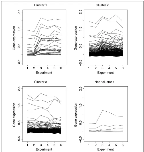
other hand, 30 genes classified into the first cluster seem to have a change in gene-expression levels. This can be verified from Figure 3, which shows the profiles of gene-expression levels across all six experiments for each cluster.
[image:6.609.52.557.84.619.2]In addition to determining the number of clusters, model-based clustering has another advantage in providing poste-rior probabilities of observations belonging to each cluster. The posterior probabilities are calculated using Equations
Figure 3
Gene-expression profiles of the four clusters found using the method described. Each line represents a single gene. Clusters 2 and 3 (containing over 95% of genes) show little change in gene-expression levels; cluster 1 (30 genes) and cluster 4 (6 genes) do show changes in gene-expression levels.
Experiment
Gene e
xpression
1
2
3
4
5
6
–
0.5
0.5
1.5
2.5
Cluster 1
Experiment
Gene e
xpression
1
2
3
4
5
6
–
0.5
0.5
1.5
2.5
Cluster 2
Experiment
Gene e
xpression
1
2
3
4
5
6
–
0.5
0.5
1.5
2.5
Cluster 3
Experiment
Gene e
xpression
1
2
3
4
5
6
–
0.5
0.5
1.5
2.5
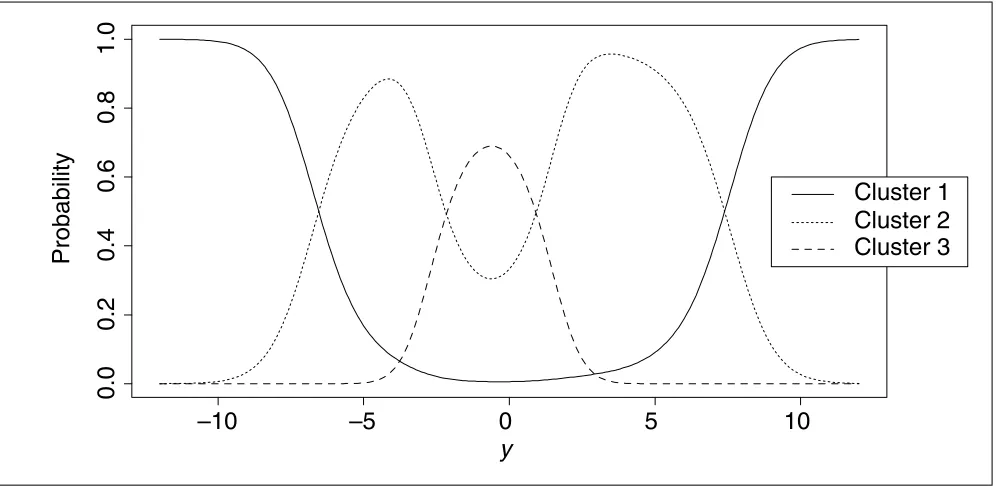
(1) and (2), and are presented in Figure 4. Recall that a gene is classified to a cluster if its posterior probability of being in the cluster is the largest. From Figure 4, it can be seen that if a gene’s t-statistic has a large absolute value, then it will be classified into cluster 1. Specifically, if a t-statistic, yi, is
smaller than -6.54 or larger than 7.39, then the correspond-ing gene iis judged to be from cluster 1. Hence, cluster 1 con-sists of genes with large absolute values of t-statistics, implying that cluster 1 corresponds to genes with large changes of expression levels (after standardization by the variation of expression levels).
Furthermore, the posterior probability can serve as a quanti-tative measurement of the strength of each gene being classi-fied into each cluster. For instance, among 30 genes classified into the first cluster, there are respectively 17, 18, 20 and 21 genes with a posterior probability of being in the first cluster greater than 0.99, 0.95, 0.90 and 0.85. Hence, those 17 or 18 genes are likely to have expression levels sig-nificantly different from those of other majority genes. The posterior probability might also provide information about possible misclassifications. In addition to those classified into cluster 1, there might be other observations classified into the other two clusters but nevertheless with not too small probabilities of being classified into cluster 1. The lower right panel of Figure 4 shows six such observations, all belonging to cluster 2 but with probabilities of being in cluster 1 ranging from 0.30 to 0.48. These six genes show somewhat differential gene-expression levels, but the
evidence is not strong and more experiments may be needed to verify this.
We hope we have shown that model-based clustering is a powerful method that is useful in analyzing gene-expression data. It is flexible as well as intuitively understandable. However, it does have some limitations. Although it provides posterior probabilities for classification results, in the context of detecting differentially expressed genes its use is more in the line of exploratory data analyses. For instance, in our example, we treat cluster 1 as representing genes with changed expression whereas clusters 2 and 3 consist of genes without expression changes. Although this treatment is reasonable, it is somewhat subjective and is debatable. Some new statistical approaches [31-33] are interesting alternatives that provide a more quantitative answer to detecting genes with altered expression, but they require replicates of spots or arrays. Model-based clustering is less restrictive and can be applied to data without replicates and to cluster (relative) gene-expression levels directly [13].
Materials and methods
Three young pathogen-free Sprague-Dawley rats were inocu-lated with pneumococcus in phosphate-buffered saline (PBS) and served as the pneumococcus group. Three other rats inoculated with PBS served as controls. All animals were sacrificed on day 42 after inoculation. The bullae from each of the pneumococcus- or PBS-inoculated groups were pooled
comment
reviews
reports
deposited research
interactions
information
[image:7.609.57.555.87.330.2]refereed research
Figure 4
Posterior probability of a gene being in each cluster as a function of the t-statistic y, calculated using Equations (1) and (2). A gene is classified to a cluster if its posterior probability of being in the cluster is the largest.
y
Probability
–
10
–
5
0
5
10
0.0
0.2
0.4
0.6
0.8
1.0
and submitted for mRNA purification. Purified mRNAs, [,-32P]dATP, dNTP mix and reverse transcriptase were
incubated at 50°C for 25 min for the synthesis of radioac-tively labeled cDNA probes. The Atlas cDNA array mem-branes (Atlas rat 1.2 array, Clontech, CA) were hybridized with the cDNA probes and nonspecific binding washed away. Specific binding of cDNA probes with the membranes was scanned into a computer and the radioactive signal intensi-ties of specific binding were quantitated with the OptiQant software (version 3.0, DeltaPackard, Boston, MA) and pre-sented in digitalized light unit (DLU). The intensity level in DLU is the observed gene-expression level. As described earlier, the log-transformation was conducted on the inten-sity level in DLU, and the centering and scaling procedures were followed using the log-transformed data. The original data representing the intensity level (in DLU) for each gene from each of the six experiments are available from our website [34].
Acknowledgements
This research was partially supported by NIH grants.
References
1. Brown P, Botstein D: Exploring the new world of the genome with DNA microarrays.Nat Genet1999, 21(Suppl):33-37. 2. Lander ES: Array of hope.Nat Genet 1999, 21(Suppl):3-4. 3. Eisen M, Spellman P, Brown P, Botstein D: Cluster analysis and
display of genome-wide expression patterns. Proc Natl Acad Sci USA 1998, 95:14863-14868.
4. Tavazoie S, Hughes JD, Campbell MJ, Cho RJ, Church GM: System-atic determination of genetic network architecture. Nat
Genet1999, 22:281-285.
5. Tamayo P, Slonim D, Mesirov J, Zhu Q, Kitareewan S, Dmitrovsky E, Lander ES, Golub TR: Interpreting patterns of gene expression with self-organizing maps: methods and applications to hematopoietic differentiation. Proc Natl Acad Sci USA 1999, 96:2907-2912.
6. Tibshirani R, Hastie T, Eisen M, Ross G, Botstein D, Brown P: Clus-tering methods for the analysis of DNA microarray data. Technical Report, Department of Statistics, Stanford University, 1999. Available at [http://www-stat.stanford.edu/~tibs/research.html] 7. Zhang K, Zhao H: Assessing reliability of gene clusters from
gene expression data.Funct Integr Genomics2000, 1:156-173. 8. Kerr MK, Churchill GA: Bootstrapping cluster analysis:
assess-ing the reliability of conclusions from microarray experi-ments.Proc Natl Acad Sci USA2001, 98:8961-8965.
9. McLachlan GL, Basford KE: Mixture Models: Inference and Applications
to Clustering. New York: Marcel Dekker, 1988.
10. Holmes I, Bruno WJ: Finding regulatory elements using joint likelihoods for sequence and expression profile data. Proc 8th
Int Conf Intelligent Systems for Molecular Biology. Menlo Park, CA: AAAI
Press, 2000.
11. Barash Y, Friedman N: Context-specific Bayesian clustering for gene expression data. Proc Fifth Annual Int Conf Computational
Biology. New York: Association for Computing Machinery, 2001.
12. Yeung KY, Fraley C, Murua A, Raftery AE, Ruzzo WL: Model-based clustering and data transformations for gene expression data.Bioinformatics2001, 17:977-987.
13. Lee M-LT, Kuo FC, Whitmore GA, Sklar J: Importance of replica-tion in microarray gene expression studies: statistical methods and evidence from repetitive cDNA hybridiza-tions.Proc Natl Acad Sci USA2000, 97:9834-9839.
14. Friemert C, Erfle V, Strauss G: Preparation of radiolabeled cDNA probes with high specific activity for rapid screening of gene expression.Methods Mol Cell Biol 1998, 1:143-153.
15. Chen Y, Dougherty ER, Bittner ML: Ratio-based decisions and the quantitative analysis of cDNA microarray images. J
Biomed Optics1997, 2:364-367.
16. Ideker T, Thorsson V, Siehel AF, Hood LE: Testing for differen-tially-expressed genes by maximum likelihood analysis of microarray data. J Comput Biol 2000, 7:805-817.
17. Newton MA, Kendziorski CM, Richmond CS, Blattner FR, Tsui KW: On differential variability of expression ratios: improving statistical inference about gene expression changes from microarray data.J Comput Biol2001, 8:37-52.
18. Dudoit S, Yang YH, Callow MJ, Speed TP: Statistical methods for identifying differentially expressed genes in replicated cDNA microarray experiments. Technical Report, Statistics Department, University of California-Berkeley, 2000.
19. Titteringto DM, Smith AFM, Makov UE: Statistical Analysis of Finite
Mixture Distributions. New York:Wiley, 1985.
20. Dempster AP, Laird NM, Rubin DB: Maximum likelihood from incomplete data via the EM algorithm. J Roy Stat Soc Ser B
1977, 39:1-38.
21. Akaike H: Information theory and an extension of the maximum likelihood principle. In 2nd Int Symp Information
Theory. Edited by Petrov BN, Csaki F. Budapest: Akademiai Kiado,
1973, 267-281.
22. Schwartz G: Estimating the dimensions of a model.Annls Statis-tics1978, 6:461-464.
23. Biernacki C, Govaert G: Choosing models in model-based clus-tering and discriminant analysis.J Stat Comput Simulation1999, 64:49-71.
24. Banfield JD, Raftery AE: Model-based Gaussian and non-Gauss-ian clustering.Biometrics1993, 49:803-821.
25. Fraley C, Raftery AE: How many clusters? Which clustering methods? Answers via model-based cluster analysis.
Com-puter J 1998, 41:578-588.
26. McLachlan GL: On bootstrapping the likelihood ratio test sta-tistic for the number of components in a normal mixture.
Appl Statistics1987, 36:318-324.
27. McLachlan GL, Peel D, Basford KE, Adams P: Fitting of mixtures of normal and t-components.J Stat Software1999, 4:2. Available at [http://www.jstatsoft.org/v04/i02/]
28. EMMIX [http://www.maths.uq.oz.au/~gjm/emmix/emmix.html] 29. Fraley C, Raftery AE: MCLUST: Software for model-based
cluster analysis. J Classification1999, 16:297-306. 30. Model-based Clustering Software
[http://www.stat.washington.edu/fraley/mclust]
31. Efron B, Tibshirani R, Goss V, Chu G: Microarrays and their use in a comparative experiment.Technical Report, Department of Statistics, Stanford University, 2000. Available at [http://www-stat.stanford.edu/~tibs/research.html]
32. Tusher VG, Tibshirani R, Chu G: Significance analysis of microarrays applied to the ionizing radiation response.Proc
Natl Acad Sci USA2001, 98:5116-5121.
33. Pan W, Lin J, Le C: A mixture model approach to detecting differentially expressed genes with microarray data. Techni-cal Report 2001-011, Division of Biostatistics, University of Min-nesota, 2001. Available at [http://www.biostat.umn.edu/cgi-bin/rrs ?print+2001]