Numerical solution of parabolic equations by the box scheme

NUMERICAL SOLUTION OF PARABOLIC

EQUATIONS BY THE BOX SCHEME

Thesis by Kirby William Fong

In Partial Fulfillment of the Requirements for the Degree of

Doctor of Philosophy

California Institute of Technology Pasadena, California

1 9 7 3

-ii-··~ _{ACKNOWLEDGMENTS}

The author wishes to thank Professor Herbert B. Keller for suggesting the problems considered in this thesis and for valuable discussions during the course of the research.

He wishes to thank also the National Science Foundation for fellowship support and the California Institute of Technology for graduate research and tea-ching assistantships.

-111-ABSTRACT

-iv-TABLE OF CONTENTS

Introduction 1

Chapter 1 The Box Scheme in One Space Dimension

I.l

!.2

I.3

I.4

I.S

I.6

I.7

Chapter 2 II. 1 II. 2

II. 3

A Basic Description of the Box Scheme

An Energy Inequality for the Heat Equation Convergence of the Box Scheme for the Heat Equation

An Energy Inequality for a Linear Parabolic System

Convergence of the Box Scheme for a Linear Parabolic System

Solving the Linear Finite Difference Equations Nonlinear Parabolic Equations

The Two-Dimensional Heat Equation The Method of Fractional Steps

The Box Scheme and the Method of Fractional Steps

Von Neumann Stability

4

10 17

28

34

44

54

69

73

-v-TABLE OF CONTENTS (Continued)

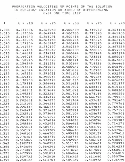
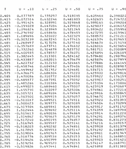
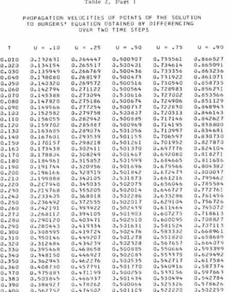
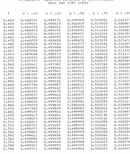
Chapter 3 Burgers' Equation: Computational Examples

III. 1 Burgers' Equation

80

III. 2 Example 1: Smoothing of a Sharp Front

84

III. 3 Example 2: Formation of a Shock

94

III.

4

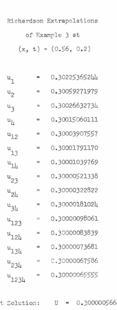
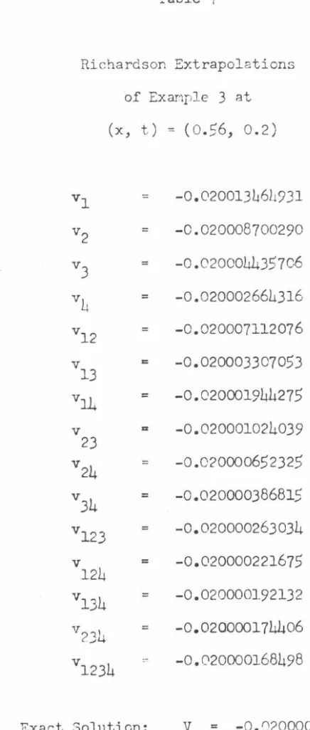
Example 3: Interaction of Two Shocks

116

1

-INTRODUCTION

This the sis deals with the numerical solution of parabolic

equa-tions by the box scheme. Chapter I is devoted to the analysis of

prob-lems in one space dimension. We begin with a de scription of the box

scheme and list some situations in which it would be preferable to

other methods of computation. We then give three convergence proofs

for the box scheme. In each proof we use discrete analogues of energy

inequalities to show that the finite difference solutions are accurate

approximations of the continuous solutions. Energy inequalities are

generally used to prove uniqueness of solutions of initial value

prob-lems; however, in our work we have used modified forms for initial

boundary value problems with inhomogeneous terms. Section I. 2 gives the derivation of such an energy inequality for the heat equation. In

Section I. 3 we show how the energy inequality can be used as a model

for. finite difference equations. We then generalize the convergence

proof for the heat equation to a linear parabolic system. Section I. 4

gives a derivation of an energy inequality, and Section I. 5 shows how

2

-yield a convergence proof of the box scheme for parabolic systems.

The emphasis of Sections I. 6 and I. 7 is on the computation of the finite diffe renee solution. In Section I. 6 we prove that an upper and lower block triangular matrix factorization may be used to solve the finite difference equations for a special linear equation. Using an argument involving principal error functions, we also show how to resolve a problem about the "smoothness" of the finite difference solution that arises in Section I. 5. Finally in Section I. 7 we give a

constructive proof that the nonlinear difference equations resulting from applying the box scheme to a particular class of nonlinear para-bolic equations have a unique solution. The mean value theorem enables us to adapt the convergence proof for linear systems to this class of nonlinear equations.

In Chapter II we give an example of how the box scheme may be extended to solving the heat equation in two space dimensions by using the method of fractional steps. We show that the initial value problem with periodic data leads to a numerical scheme which is stable in the

3

-

4-CHAPTER I

THE BOX SCHEME IN ONE SPACE DIMENSION

I. 1 A Basic Description of the Box Scheme

The box scheme for the numerical solution of parabolic equa-tions was originally proposed by Keller [1971]. Since this scheme is of fundamental importance in this thesis, we present here a brief review of the method and indicate some of the ways in which it is superior to other numerical methods for solving parabolic problems. We consider the following special problem defined in the rectangle 0 ~ x ~ 1 and 0 ~ t ~ T:

~~

=

a:

(a (x)

;~) +

c (x)U

+

S (x, t), (l.la)

U(x, 0) = g(x), (1. lb)

(l.lc)

a1 U(l, t)

+

[31 a(l )U (1, t) = g1 (t).

X (1. 1 d)

-

5-au

a(x)

ox =

V,

av

ox

=

at -

au

c (x) U - S (x, t ),

U (x, 0) = g (x),

V(x, 0)

=

a(x)

d~~)

,

a₀ U(O, t) - {30 V(O, t) = g0 (t),

a1 U(l, t)

+

{31 V(l, t) = g1 (t).

We define a mesh over the rectangle:

<

tN

=

T.

The mesh spacings are then defined by

h.

-

X.

-

_{X. J'}

J J

J-k

_-

t

-

t n-1'

n n

for j = 2, • J and n

=

2, • • • N. For net functions {

cp

~}

and coordinates of the net we use the following notation:

x.±1

J 2

t _n ±1

-2

n cp. ± 1

J 2

(1. 2a)

(1. 2b)

(1. 2c)

(1. 2d)

(1. 2e)

( 1. 2£)

(1. 3a)

(1. 3b)

(1. 3c) (1. 3d)

(1. 4a)

(1. 4b)

-

6

-n ±.l

t(

_{n n±l)} cp. 2 _{- 2 cp.}

+

_cp. 1

J J . J (1. 4d)

n n

n cp. - cp. 1 D cp. - 1 ]

-X _J h.

J

(l.4e)

n n-1 n cp. - cp. Dt cp. - J J

k

J _n (1. 4f)

For functions \jt{x, t) defined everywhere in the rectangle we use the notation

t~

-

\jt(x.1 t ) 1

J . J n (1. 4g)

n \jr. ± 1

t (x. ± 1 t ) 1

J 2

-

_J

21 n (1. 4h)

1

t~±2

_-

_t (x.1 t ± 1 ).

J J n 2 ( l. 4i)

The box scheme for the numerical approximation of problem (1. 2) is given in terms of the net functions [u~} and

J [ v~} J with all the dif-ference approximations centered in the middle of the box

[x.

1• x.] X [ t 1• t ] or on

an

appropriate edge of the box when

J- J n- n

coefficients do not depend on the time variable. We have

a. 1 D J-2 x

1 - n-2 D v.

X J

n u. J

for 2 ~ j ~ J and 2 ~ n ~ N. The initial data are taken as

(1. 5a)

7

-l

=

g (x.) • u.

J J (1. Sc)

1 d g (x_J .)

v.

₌

a. dx

J J (1. Sd)

for 1 ~j ~ J, and the boundary conditions become

n

- i3o n n (1. Se)

ao ul vl = _{go •}

n n n

( l. 5£) Q'l _UJ

_{+ f}l}

_{VJ =} gl •

for n ~ 2 ~

N.

We immediately see two advantages of this method over other

numerical methods which have been proposed. First the mesh

spacings need not be uniform so that we may use a finer net in regions

where we expect rapid changes in the solution. Second, the scheme

is well adapted for problems in which a(x) is not continuous. For

instance in a diffusion problem where a(x), the diffusivity of the

medium, is dis continuous,

~~

. will also be dis continuous, but the

flux a(x)

aa~

which is one of the dependent variables in the box scheme will be continuous so that we need not make any special modifications

for discontinuous coefficients other than to pick the points of

dis-continuity to be mesh points.

There are other desirable features which are not so apparent.

Being implicit, the method will be unconditionally stable. The method

has second order accuracy even with nonuniform nets. Richardson

8

-differentiable and yields an improvement of two orders of accuracy for each extrapolation. Both U(x, t) and oU(x,

_ox

t) are approximated to the same order of accuracy. Although the box scheme requires a little more computation than the Crank-Nicolson scheme, it will nevertheless be preferable for the types of problems described in the preceding paragraph.

-

9-goal is to enlarge the class of parabolic problems for which we can

guarantee convergence of the box scheme. We shall give a different

proof for the convergence of the box scheme for the heat equation and

then show how it can be extended to a parabolic system and to a class

of nonlinear parabolic equations. There will be some mild restraints

on the net spacing, but basically we will be allowing nonuniform time

and space steps.

Implementation of the box scheme will entail the solution of

linear systems of algebraic equations. While stability or convergence

will imply that the systems are nonsingular and have unique solutions,

it still remains for us to chaos e an appropriate algorithm for obtaining

these solutions. In general an algorithm for solving a linear system

will require that further conditions be satisfied in addition to

non-singularity before we can prove that it will produce the desired

solu-tion. We shall use the method of factorization of block tridiagonal

matrices recommended by Keller [1971]; however, we shall give an

alternative proof based on an analysis suggested by Varah [ 1972] that

- 1

0-I. 2 An Energy Inequality for the Heat Equation

The convergence proofs which we shall present are based on

energy inequalities. Energy inequalities are often used to prove

well-pos ednes s of initial value problems or to show that a solution depends

continuously on the initial data of an initial value problem. It is

frequently possible to construct a dis crete analogue of an energy

inequality which can then be used to prove convergence of a finite

difference scheme. Indeed, this is how we shall obtain our

conver-gence proofs, and to this end we wish to study thoroughly a simple

parabolic equation - namely the heat equation - beginning with an

energy inequality.

We consider the following problem:

v

=

u

x' (2. l a)

v

_X

=

ut • (2. 1 b)

U(x, 0)

₌

g (x) • (2. 1 c)

V (x, 0)

=

d g(x)

dx (2. 1d)

a0 U(O, t) - ~0 V(O, t)

=

go (t) , (2. 1 e)

a₁ U(1, t)

+

~₁ V(1, t)

=

g1 (t), (2. 1 f)

1 1

-o.

(2. lh)

The conditions (2. lg) and (2. lh) are physically natural requirements

for a mixed boundary condition. If these quantities are for some

reason less than zero, our energy inequality would contain integrals

along the boundaries x

=

0 and x

=

l. With the present assumptions

these integrals will have signs such that they can be dropped from the

inequalities we will derive. The case of Dirichlet boundary conditions

where {30 or {31 is zero is actually simpler than the mixed case and

would require only minor modifications of the proof. We therefore

consider only the mixed cas e.

Typically, an energy inequality argument is used when one

wishes to show problem (2. 1) has a unique solution. If we assume

U and V are one solution pair and u and v are another solution

pair and define the difference functions

e (x, t) - U (x, t) - u (x, t) , (2. 2a)

f(x, t) - V(x, t) - v(x, t), (2. 2b)

we find that e and £ are solutions of

f

₌

e

X (2. 3a)

f

=

_{et '}

X (2. 3b)

1 2

-f(x, 0)

=

0 , (2. 3d)

ao e(O, t) -

f3

0f(O, t)

=

0 , (2. 3e)

al e (l, t)

+

f3

1 f(l, t)

=

0 , (2. 3f)

ao

~ ;e: 0 , (2. 3g)

al

~

:2: 0 . (2. 3h)

One then notes that the integrals with respect to x of the squares of

e and f are zero at time zero and must be non-increasing functions

of time. Since these square integrals are non-negative, they must be

zero; therefore, e and f are zero for all time, and the solution

pairs must be identical. This, however, is not the manner in which

we wish to use the energy inequality. Let us suppose instead that

u and v satisfy (2. I) but that U and V satisfy only the boundary

conditions (2. le) and (2. 1£). Then we would have the following

rela-tions governing e and f:

e

₌

f

+

p , (2. 4a)

X

f

₌

X et

+

a , (2. 4b)

ao e (0, t) -

f3o

f(O, t)

=

0, (2. 4c)

al e(l, t)

+

f3

1 f(l, t)

=

0, (2. 4d)

ao

1 3

-al

13;

;;;:: 0 I (2. 4f)

p - u

- vI

(2. 4g)

X

(J _-

v

_{- ut. (2. 4h)}

X

The terms p and

a

account for the fact that U and V do not

necessarily satisfy the differential equations. Before proceeding

with the derivation we should like to furnish some motivation by saying

that in the finite difference problem u and v will be solutions of the

finite difference equations while U and V will be the solutions of

the continuous system we are modeling. That is, u and v are to

be the computed approximations to U and V. Since the difference

equations are only approximations to the differential equations, we

cannot expect U and V, the solutions of the differential equations,

to satisfy the difference equations exactly. The extent to which they

fail to satisfy the difference equations is embodied in the truncation

errors p and

o.

The terms p .and

a

are generally small. Specif-ically, for the box scheme, they are 0 (h2). Usually e and f are

zero at time zero, but we shall not assume this. With this

interpre-tation of the various terms in (2. 4 ), we see that the results we need

are bounds on e and £ at times greater than zero in terms of p, a,

and the initial values of e and f. This is called a convergence

result because p and a can be made arbitrarily small by taking a

sufficiently fine mesh and because the initial error also can

- 1

4-the mesh is refined, 4-the finite difference solution must converge to

the continuous solution.

Our plan is to derive an energy inequality from (2. 4) and then try to duplicate the derivation for a discrete system. It turns out that it is convenient to take the time derivative of (2. 4a):

(2. 4i)

If we multiply (2. 4i) by f and (2. 4b) by e. add the products, inte-grate with respect to x from 0 to 1, and make a substitution using

l 2

(2. 4a), we obtain, with (cp,

'f)

=

/

cp(x)t(x)dx and

II

cp

II

== (rp, rp) ,

0

1 d 2 1 d 2 2 dt lie

II

+ 2 dt llfll

./

(e. a)

1 J l (2. 5)

+ [f et]o - (fx• et) + [e f]o - (f, f) - (p, f).

Further substitutions, a careful examination of the boundary conditions, a time integration from 0 to

t,

and the Schwarz inequality lead us to

t

~

c

+ 2

I

t

II

f

II ·II

Pt

II

+

II

e

II • I

Ia

II

+

II

f

II

·llall

0 X

(2. 6)

+llfll·ll Pll }ds,

where

- l

5-We recognize that on the left side of (2. 6) we may change t to T

without destroying the inequality provided 0 ~ T ~ t. Then we

inte-grate both sides with respect to T from 0 to t. Also the four terms

on the right side of (2. 6) may be separated using the generalized

arithmetic-geometric inequality ab

~

·h

e

a 2 + .!_ b2} where

e

is an

€

-1

arbitrary positive number. In two cases we take e

=

(2t) , and in

the other two we take €

=

(4t)-1• We then find

t t t

f

f

llell2 ds -

i f

II£ ll2ds

~

C t + 2 t2

f

lloll2 ds

0 0 X 0

t t (2. 8)

+ 4t2

f

IIPII2ds + 4t2

f

lloll2ds.

0 0

Starting again with (2. 6) we find a judicious use of the generalized

arithmetic -geometric inequality gives

t

lle(t)ll2 + ll£(t)ll2

~

C

+

{i

/ llell2ds

. 0

t t t

- i f

II£ ll2ds}

+

f

11Ptll2ds + -₃8

f

l!oll2 ds

0 X 0 0

(2. 9)

The final energy inequality results from substituting (2. 8) into the

braces in (2. 9):

t

lle(t)ll2 + ll£(t)ll2 ~ C(l+t) +

f

11 Ptll2ds 0

t

+(~+6t

2

_)/

lloll2ds

·

o

t

+ (l+4t2 ) / IIPII2 ds.

0

- 1 6

-If we restrict t to lie between 0 and T, we see that the three terms

involving the truncation errors can be bounded independently of t.

Referring to (2. 7) we note that C is determined by the initial errors

and can be made small. Hence the energy inequality (2. I 0) is in the

form we need for a convergence proof of the difference equations.

The derivation given in this section was c;uggested by Lees

1 7

-I. 3 Convergence of the Box Scheme for the Heat Equation

Let [u~} and [ v~} be net functions which we shall use to

J J

approximate U and V respectively. The box scheme for the heat equation then takes the form

n

v. 1

=

J-z

1

D- v~-z = X J

l u. J l v. J "'o Q'l "'o

~

Q'l

=

=

n - l3o ul n

UJ

+

j3l

~ _0,

- n

D

u.

X J

- n

Dt u. 1 ,

J-z

g (x. ), J

dg (x.)

J dx

n vl

=

n

VJ

=

n go ,

n gl

13;

~ 0 .

Let U and V be the solutions of (2. 1) and define the error net functions

n

U(x., t ) n

e.

-

- u.

'

J J n J

f.l

_-

V(x., t ) - v. n

J J n J

(3. la)

(3. 1 b)

(3. 1 c)

(3. ld)

(3. 1 e)

(3. If)

(3. 1 g)

(3. lh)

(3. Za)

1 8

-[e~ } and t£~} are then solutions of

J J

D- e~

=

f~ I

+

p~ 1 ,

X J J

-z

J

-z-1

- n

n-z-=

Dt e. 1 + 0. r ,

J

-z-

J

-z-el:

=

0 , J

f

l:

= 0 ,

J

n

+

f31 0:'1 _eJ

O:'o

~

;;:: 0 '

0:'1

K

;;:: 0

fn

0 '

=

J

where the local truncation errors are defined by

{

_ 8U(x._.!_, t ) }

p~ 1

=

D U(x. t ) - J z n

J

-z-

X j' n 8x

+ {v(x.

1, t ) - t[V(x., t )

+ V(x.

1, t

>J},

J -z- n J n J- n

1

n-z- {

a. I

=

t D- [V(x., t )

+ V(x.,

t

1)]

J

-z-

x J n J

n-- t Dt- [U(x., t )

+

U(x. l' t

)J} .

J n J- n

(3. 3a)

(3. 3 b)

(3. 3 c)

(3. 3d)

(3. 3e)

(3. 3f)

(3. 3 g)

(3. 3h)

(3. 3i)

- 1

9-If we apply the operator

n;

to (3. 3a), we obtain

where

1

n-z-( . ₁ is defined by J-z

1 n-z- [

( _. 1 - vt (x. _{J --;-}1, t _n--;-1 )

J -z- c. c.

- n }

Dt V. 1

J-z

+ [

Dt- D- U~ - U t (x. 1, t 1 ) } •

X J X J -z-

n-z

(3.3k)

(3. 3 J,)

It is possible to give alternate expressions for the truncation errors if we use Taylor expansions in the above definitions. First, however, we wish to introduce some new notation. Let h

=

max h. ,

j J Let 8 (x) and cp(t) and for some fixed r

>

0 we assume max k

=

rh.

n

n

be piecewise continuous functions such that for some fixed 5

>

0 we have

h.

J = 9 (xJ-z-. 1 )h,

}

(3. 4a)

~

e

(x) ~ 1 , O ~ x ~ l,

2

~

n

~

N.}

O ~ t ~T.

k

=

cp(t !)h,

n

n-z-(3. 4b) 6 ~ cr:(t) ~ r ,

where

I

n--z

a. 1

J-2

=

=

=

- 2 0-2\J

~

(h

2 ) R [U,V;x. 1,t }+O(h

2

m+2),

'J=l \! J--z n

m (h )2\J f } 2m+2

~

-2 S 1..U,V;x. 1,t 1 +O(h ),

\J=l \! J --z n--z

m (h )2\J 2m+2

~

-2 Z [ U, V ;x. 1, t 1 }

+

0 (h ),

\!=I \! J --z

n-z-e

2_{\J( ) { I a}2

\J+ I U(x, t)

R [U, V;x, t}

=

__

x • -

-\! (_{2 \J)!} 2\J+I • ax2'J+I

2\J

_ a

vJ~·

t)} .

ax

2/l

8 2\)- 21-L

\! cp (t) . (x)

S [U,V;x,t)}

=

~

\! 1-L=O (2/l)! (2\J- 2J.L)!

I a2\J+I U(x, t)

~

ax2'J-2/l at2/l+I ) '

\) 2\)- 2/l ₈ 2/l

_

~

cp (t) (x)

1-L=O (2/l)! (2'J-2/l+l)!

Z\! [V, V;x,

t}

(3. Sa)

(3. Sb)

(3.

s

c)

(3. Sd)

(3. Se)

(3. Sf)

For the purpose of this section the most important feature of the

truncation errors is that all three errors are O(h2 ).

We next introduce an inner product for net functions

and [ \fr~}:

J

:6

n

CfJ. I j =2 J

-z

2 l

-n

\jr. I h .. J

-z

J

If a net function is differenced, we will have J

n - n

:6

cp. 1. D \jr. h ..

j =2 J-2 X J J

The norm associated with this inner product is

n n (c:p ' cp )h.

(3. 6a)

(3. 6 b)

(3. 6 c)

We note that (3. 6c) is actually a seminorm rather than a norm since a net function which oscillates along the mesh can have norm zero without itself being zero. We shall say more about this after the

convergence proof. Finally, with our inner product the following identities hold:

(3. ?a)

(3. ?b)

As mentioned earlier our plan is to construct a dis crete

2 2

-1 1

1 _-

II

n

ll

2 1

-

ll

...n

ll

2

...n.-2

n-

2

2 D t e h

+

2 D t 1 h

=

- (

1 ,

C

)h (3. 8)

1 1

( n-2 n-2)

- e ,

a

h

Beyond equation (3. 8) the discrete nature of the variables causes

some difficulties which did not occur before. We therefore

intro-duce new quantities which will help us notationally:

kl

-

k2'

1

llf

2

_llh

_-

_{0 ,}

1

IIC

2

₁₁

_h

_-

_{0 ,}

1

li

n~

f

2

_l

_l

_h

₌

_o,

1

llo

2

_ll

_h

1

IIP

2

_IIh

s m

-

0 ,

-

0 ,

(3. 9a)

(3. 9b)

(3. 9c)

(3. 9d)

(3. 9e)

(3. 9f)

(3. 9g)

- 2

3-This notation plus additional substitutions, careful examination of the

boundary conditions, a time summation from t1 to t , and the Schwarz _n

·inequality lead to the analogue of (2. 6):

(3. 1 0)

1 n

+

ll

fm-

2

11

h2 )

~

C

+

2

:6

k •

m=l m

where

(3. II)

We see that on the left side of (3. 10) the index n may be changed to i

where 1 ~ i ~ n yielding a set of valid inequalities. We then multiply

both sides by k. and sum from i = 1 to i = n. We again apply the

1

arithmetic -geometric inequality to each of the four products on the

right side of (3. 10). With the notation D

=

t

+

k1 we now obtain

n

+

2 D2 .6 k s2 m=l m m

-24-(3. 12)

(3. 12) corresponds with (2. 8) but has additional terms in

ll

fml

l

~

and .!. 2

llfm-2_{llh because a cancellation which occurred in the continuous case} does not occur for discrete equations. Returning to (3. 10) we use the arithmetic -geometric inequality with different parameters to deduce

(3. 13)

n 2

max l~m~n

we conclude the result

2

T ,

m

- 2

5-3 2

+ [(t +k_n 1 ) + t +k_n 1 ] T (n) .

(3. 14a)

(3. 14b)

(3. 15)

(3. 15) is the convergence result we sought. It says that the errors at

a given fixed time may be made small if the initial errors are small and if the truncation errors are small. The latter error we noticed

earlier was O{h2 ) and can be made smaller by refining the mesh. We

note also that km+l /km is bounded by r

I

6; hence, no further condi-tions are needed to guarantee that T (n) is 0 {h2 ). If the initial data are approximated to O{h2) or better, then we see llenllh and llflllh

are also O{h2 ).

There remain two points which must be clarified. The first is to show that there exists a unique solution of the finite difference

problem (3. 1 ). We shall defer this to a later section. The second is

- 2

6-explanation here since possible oscillations in the finite difference solutions are of concern in practical computation.

Two net functions fcpj} and

t

tj} satisfy jjcp- tJJh = 0 if and only if

cp.

= t.

+ (

-1 )Jp for some constant p. Thus if lien -~Jjh = 0

J J

and jjfn-Tnjjh = 0, there eXist p and q such

that~= e~

+

(-l)j p

J J

and f.n = f.n

+

(-l)j q. In order that fe.n}, tf.n}, r;;·_n}, and ff.n}

J J J J J J

satisfy the boundary conditions we must have

ao P -

13o

q

::}.

(3. 16)

Four cases can occur. First, if a0

13

1

+

a1

13

0

f:

0, then p = q = 0, and the seminorm is actually a norm for net functions satisfying (3. 3e) and (3. 3f). Second, if

13

0

13

1 = 0, then p = 0 so that fv.n} but not

J

f u.n} may have oscillations. Third, if a0 a1 = 0, then q = 0, and J

[u~} may have oscillations. Finally, none of the above may happen J

so that both fu~} and

J f v~ J } could have oscillations. In the latter cases oscillations are eliminated by averaging neighboring values. Define

-n 1 n n

(3. I 7a) u. 1 - z-{u.

+

u. 1 ),

J-z

J

J

-- n .!. n n _{(3. I 7b)}

v. 1

-

2 (v.

+

v. ₁) ,

J-z

J J

-for 2 ~ j ~ J. Then Jjli"njjh = Jjunjjh and Jj-;; njjh = JJ vnjjh, but now

- 2

- 2

8-I. 4 An Energy Inequality for a Linear Parabolic System

We now wish to extend our analysis to a larger class of

para-belie equations. Consider the following problem:

A2 (x) U (x, t) = Y._(x, t), -x

Yx(x, t) = !:\(x, t) - C(x) Q(x, t)

- E(x)

y_

(x, t) - ~(x, t) ,

Q(x, 0)

=

g_(x)'

y_

(x, 0)

dx

a0 Q(O, t) - f3o Y._(O, t) = _[o (t),

0'1 !:!(1, t)

+

!31 Y._(l, t)

=

[1 (t)'

-1 -1

f3₀ and !31 exist ,

2 -1 -1

A (O)f30 a0 and ~(1)!31 a1 are positive

semi-definite and symmetric,

A(x) is symmetric and positive definite uniformly in x

(4. la)

(4.lb)

(4. lc)

(4. ld)

(4. l e)

(4. 1 f)

(4.lg)

(4. lh)

(4. li)

Here

Q,

~ ~(x, t), g__{0 ,} and [ 1 are vectors of dimension p and A(x), C(x), E(x), a0 , f30 , a1 , and !31 are p Xp matrices. The

domain of the problem is 0 ~ x ~ 1 and 0 ~ t ~ T. Condition (4. lh)

has been imposed so that boundary integrals which will arise will have

- 2

9-they would otherwise have to be retained. (4. lh) is a convenient assumption but not an essential one.

We now seek an energy inequality which we can use as the basis for a convergence proof. As before we suppose

£

and v are functions which satisfy the differential equations, the initial conditions, and the boundary conditions. Let U and

y_

be another pair of func-tions which satisfy only the boundary conditions. We define

~(x, t)

f_(x, t)

We find that

A2 e

f

- x -x

e

-

:Q(x, t) £(X, t) 1

- y_(x, t) ~(x, t)

and f satisfy

=

.f+_e,

=

~t C e - E f

+

£_,

f

+

~.' - t

-a0 ~ (0, t) - [30

.£

(0, t) = Q_,

0

(4. Za)

(4. Zb)

(4. 3a)

(4. 3b)

(4. 3c)

(4. 3d)

(4.3e)

(4. 3£)

(4. 3g)

- 3

0-p_,

£_, and .G_ are error terms resulting from the fact that U and V do not necessarily satisfy the differential equations. If we take the

dot products of ..[ with (4. 3c) and A2 ~ with (4. 3b), add the results, integrate over 0 .,;; x .,;; 1, and integrate by parts, we arrive at

(4. 4)

1

- (A2

Lx'

~t)

+

[A2e • f

Jo -

(AxA ~ ..[)

-

(AA

e, f ) - (A 2 e , f ) • x - - - x

-We introduce the notation

\\

A\

\

for the maximum for x

E [

0, 1]

of the

Euclidean norm of the matrix A(x). Let E: be the positive arbitrary

parameter in the generalized arithmetic-geometric inequality. Define

constants K, C1 and C 2 as follows:

K - 2 max { 1

+

1-

\\ACA -1 \\

2

+

1-

\\ Ax \\

2

\\AE\\ 2

+

\\E\\ 2

+

1

+

2\\Ax\\

2

+

~

\I

AA)

\

2

+

(3;e) \\AxA

\

\

2},

c l -

~

-

~

\

\A

-1

\\ 2

'2

C

2 -

2

+

4

\\

A\

\

.

(4. Sa)

(4.5b)

3 1

-We next make substitutions using (4. 3a) and (4. 3b), simplify (4. 4)

using the boundary conditions, the Schwarz inequality, and the

gen-eralized geometric inequality, multiply both sides of (4. 4) by the

inte--Kt

grating factor Ze , and integrate both sides from 0 to t:

2 2 t 2

II

A~(t)

ll

+ ll.£(t)ll +

f

eK(t-s) (ZI[i(s)ll 0

2 2

+ Cl i!Al_x(s)ii )ds

~

eKt(ii A

~(O)

il

2 t { 2

+ il£(0)11 ) + /eK(t-s) C211£.(s)li

0

+

Z

II

A~(s)

li

·

II

A

£

(S)

II

+ Zlli_(s)ll ·< li

~

(s)

ll

+ ll.eJs)li) + 2[A2(x)_£(x,

s)·~(x,

s)]

1 } ds 0

(4. 6)

We have assumed € has been chosen so that C₁ is positive. In further

I

I

simplifying the boundary terms it will turn out that C₃ , another constant,

arises naturally:

2 -1

- A (0)

!3

0 a0 ~(0, 0)·~(0, 0) (4. 7)

2 2

+ IIA~(O)II + lli_(O)il .

Inequality (4. 6) is also valid if we replace t by T on the left side and

if 0 ~T ~ t. We integrate T from 0 to t, simplify the boundary

- 3 2

-t 2 2

I

(II Ae(s}ll +II f(s)ll )ds s; 2 c3 t eKt

0 -

-t 2

+ 4 t eKt

I

e -Ks c2 II £_(s>ll ds

0

2 t 2 2 2

+ 2 t2 e Kt

I

e- Ks CIIAo(s}ll + 2 11 C(s)

II

0 -

-2

+ 2 II P (s)

II

Jds .

(4. 8)

Inequality (4. 6) may also be reduced using the geometric inequality

to

t

+ eKt / e-Ks {c211£(s)ll2 + e-KsiiA £(s)\12

0

+ 2e-Ks llf._(s)\12 + 2 e-Ksll _e_(s)\12} ds

+ e Kt { / ( II

A~

( s ) II + \1 !_( s )

II

G )d s} .

0

Inequality (4. 8) is now substituted into the braces in (4. 9):

+2eKt(l _{+ 2t 2 e 2Kt)}

I

t e -2Ks _ll<:(s)I!Gds 0

+ 2eKt(l _{+ 2e e2Kt)}

I

t e -2Ks _{ll_e(s) 11}2 _ds 0

(4. 9)

3 3

-(4. 1 0) is the desired form of energy inequality. It tells us that e

and f can be bounded for a fixed time t in terms of 0 _Q, ~ and

c

3

which depends on the initial conditions.

In conclusion we give a brief summary of the technique of

energy inequalities as used in our work. One first derives a

differ-ential inequality for suitable variables such as

~

~ ~(t)

ll

2

+

ll_!.(t)ll2•

The differential inequality is solved in the manner of Gronwall's

in-equality. This process can be used both for continuous and discrete

equations, but since the dis crete case tends to be more complicated,

- 3

4-I. 5 Convergence of the Box Scheme for a Linear Parabolic System

In this section we wish to analyze the convergence of the box

scheme applied to problem (4. 1) using

a

dis crete analogue of the

energy inequality derived in Section 4. Let {u~} and

J

functions approximating

Q

and

Y.

the solutions of (4. 1 ). We make

the same assumptions on the matrices as before -namely (4. lg),

(4. lh), and (4. li). The finite difference equations are

1

D- v~-2

=

X - J

l

u .

=

- J

l

v.

=

- J

1 n-2

- E. 1 v ₁

-J -2 - j -2

g_(x.)' J

d g_ (x.)

A2_{(x.) J}

J dx

1 n-2

s .

1 '

- J-2

n n

.[o (tn) '

ao ~~

-

f3o ::0

=

We define the errors

U(x., t ) - J n

g (t ) . :::J. n

n

V (x., t ) - v.

- J n -J.

(5. la)

(5. 1 b)

(5. 1 c)

(5.ld)

(5. 1 e)

(5. lf)

(5. Za)

The errors

I

- n-2

D

f .

X -J =

- E. 1

J-2

- 3

5-r fn. } t" f

1. sa 1s y - J

f~ I

+

0~ I - J -2 J::..J -2

I

n-2

f . I

J-2

I

n-2

+

0. 1

J-2

1

n n-2

=

Dt- f . 1

+

£. .

₁

- J -2 J -2

=

Q_,

(5. 3a)

(5. 3b)

(5. 3 c)

(5. 3d)

(5.3e)

where

{.e.~

.!.} •

{

a

~-}}.

and

]-2 ) - 2

{

C

_-J-2

~-t}

are truncation errors. As

in the case of the heat equation, they will all be 0 (h2 ). In place of the

function exp(-Kt) we will use its discrete analogue:

gl - 1 •

}

=fr

( 2-K k ) n

g (t )

2 +K k : for n

~

2 •

g

-n

m=2

(5. 4)

where k

<

2/K for all m. m

1

n-2

We begin by taking the dot products of

l.J·

.!.

with (5. 3c) and

1 - 2

n--A~

.!.

~- ~ with (5. 3b), adding the products, multiplying by h., and

J-2 J -2 J

summing from j = 2 to j = J. We would like to sum by parts

1

D- f n- 2 ) but now we are faced

x - h'

1

3 6

-I at x . .!. and multiplying by the averaged value of

~-z-J-2. I

-t

n--

n--rather than averaging A 2 (x.

1) f. 1

2 _{and A} 2

(x.) f. 2_•

J- -J- J -J The summation

by parts formula (3. 7a) requires the latter quantity. In order to

n-.!. I

proceed we shall reinterpret A2

1.

2 _{and A}2

en-z- to fit the formula,

I I

but we shall then have to accept new terms wn-z- and y_n-z- which account for the difference between the terms we actually have and the terms we need for summation by parts.

1 n-

-An analysis of

Y':!

2 I

n--and y_ 2 _{is not needed now so that it will be postponed to a later}

I I

section. At the present time we simply accept :y;:n-z- and .:yn-z- as net functions which make the following modified summation by parts formulas true:

(5. 5a)

(5. 5b)

3 7

-(5. 6)

I 1 J

n-z-)

+

[A2 fn-z-. D- n

J

2

h - t

~

1

As a result of the modified summation by parts formulas, the A2 in the next to last term on the right side of (5. 6) means the average of A2 (x.) and A2 (x.

1) rather than A 2

(x. 1 ). Thus we cannot use

J

J-

I

J

-z-(5. 3a) to substitute for A 2 D- en-z- in this term. As a matter of x

-fact, we really should have a different notation for this A 2 since it has a different meaning in this term than in the other terms of (5. 6 ). Define

A.2 I

-

z-(A (x.) I 2

+

A 2 (x. 1) ),

J-z

J

J-

(5. ?a)

X.

I -

~

J-z

J

2 (5. ?b)

,._,n

We define _£. I by means of

J-z

A~ I D e. n

=

~ I

+

-n £. . I

- 3 8-We claim now that

---n n 2

.e_.

1

=

p. 1

+

O(h ), (5.9)

J-2 - J-2

although the proof will be postponed. The validity of (5. 9) depends both on the smoothness of A2 (x) and the (yet to be defined) ''smooth-ness'' of the [e~}. We add at this time that the terms containing

1

-

t

~n-2 _{and :tn-2; will also require "smoothness" on the part of the}

finite difference solution. These points will be fully discussed later. Define two constants K and C1 by

K

=

max { [2

+

\I

ACA -

1 112

+ II

ACA-

111

2

+ l

lcA-

1

11

2

+

II

(D~A

2

_)A-

1

II

2

J.

[

II

A-

1

D~

A

2

l

l

+

II

AE

II

2

+

I

IX E

ll

+

311

D~

A

2

ll

2

+l+IIEIFJ} .

cl

=

l+

II

X

II

2•

(5. lOa)

(5. lOb) Substitution of (5. 3b) and (5. 8) into (5. 6) followed by applications of the Schwarz, arithmetic -geometric, and triangle inequalities and

1

multiplication by 2 gn-2 yield

-39-Let

2 -1 1 1 2 -1 1 ,

A (O)f3o ao!:1·~1 ·+ A (1)[31 al~J·~J

+

I

~ ~

1

II

~

+

1

1

.£

1

II

~

.

(5. 12)

Then a time summation of (5. 11) and an analysis of the boundary terms lead to

g

Let k1 - k2 and define

1 C2

n (5. 13)

(5.14)

-40-(5. 15)

t C2 (l +C3)

n +C

n 3

g

+

(ym--z D- fm--z) 1 1

J

- • x - h

+

(5.15) corresponds to (4. 8). To find the discrete version of (4. 9) we

return to (5. 13) where we estimate the terms involving truncation

errors with the arithmetic-geometric inequality:

:;;; _1_

c

n 2

g

-41-The terms in the last set of braces are estimated with (5. 15 ). Suppose

we define

=

max -f ,

2::;m ::;n m

0

max~

:n

(I

Then the final inequality may be written as

2 -1 1 1

l

+

A (I) f31 a1 ~J • ~J

J

(5.17a)

(5. 1 7b)

(5.17c)

-42-(5. 18) tells us that the error at time t can be bounded by an

ex-n

pression involving three types of quantities. The first type consists

of the errors

{~j}

and

{Lj}

made in the initial values. The second

type consists of {wr:-}} and

{v~-f}

combined with

{e~

IJ_ and

{f~L

-J-z

..cJ-z

-J

-JJ

which arose when we summed by parts two terms for which the

summa-tion by parts identity was not really valid. The third type involves the

truncation errors {

Q_T-i-~J,

{

~i}

and

{£.~t}

.

It is clear that

the first type of term can be made 0 (h2 ) by a sufficiently accurate

approximation of the initial condition.

if the {

£:j~t}

do not differ from the

The third type will be O(h2)

{

.e_j-tf

m

I

bymorethanO(h )as 2

has previously been claimed.

1

We must investigate further the net

{

} {

m-·n

functions

£.j~t

,

Y:j

-t

J

,

and

{

y_

m-tl

j

-t

J

.

We start with {

£.~

.!.} It can be shown by Taylor series

ex-J-z

pansions and (5. 3a), (5. 7a), (5. 8), and (5. 9) that

h.a

= m _.L_

0 - 1

+

8

J:;__J

-z

D X

n e. '

J (5. 1 9)

where

S·

1 is some point between x.

1 and x.. If the second

J-z

J- J

derivative of A2 (x) is uniformly bounded and if D- e~ is 0(1 ), then

1 X - J

the {£:.m.!.} will be O(h2 ). As for the {w:ni2} and

J-z

-J-z

₁

{ m-z}

treatments are similar so we shall consider w. 1

-J-2

{ m-t}

y_.

.!. , their

J-z

alone. Again

-43-1 1

..n_

-z-

n-z-.!.1.

+

i]· -

1

A 2 (x. 1 ) • - -

=

J-z: 2

(5. 20)

2

h. 8 A2 (x. I)

+

_l. • J

-z-4

ox

1

n-z:

w. 1

-J-2 is defined as all the terms on the right side of (5. 20) except

.!. n-1.

the first one. The same definition holds for y_~-

i

with f. 2

re-1 J

-z

-J 1

placed by ~-2• If D-e~ and D- f~ are 0(1), then

wr:-1

and

J X "J X- J

-J-z

y_

r:-}

will be 0 (h2 ). Furthermore, the {w

~ii}

and { y

:n1:i}

:J-2 -J-2 J-2

- - n

occur in inner products and time summations with D Dt e . and

X -J

- n

D f . . These latter must be 0(1) to guarantee that our terms of

x- J

the second type be 0 (h2 ). If U and V are continuously differentiable

in x and the cross derivative of U is continuous, then our three

- n - n - - n

conditions are that D u., D v ., and D Dt u . be 0 (1) as h ... 0

X -J X -J X -J

for {

~j}

and {

~j}

solutions of the difference equations. We shall

-44-I. 6 Solvin~ the Linear Finite Difference Equations

Problem (5. 1) may be written as a block tridiagonal linear

algebraic system of equations with Zp X Zp blocks. We would like

to show that factorization into upper and lower block triangular

matrices can be used to solve this syst~m; however, we currently

have a proof only for the case p

=

1. In this section we restrict

ours elves to an equation with constant coefficients and a net with

uniform space steps h and uniform time steps k. In the next

section on nonlinear parabolic equations we will generalize the proof

to include variable coefficients and nonuniform meshes. After we

show that the finite difference solution exists and is unique, we can

show that it is "smooth" in the sense described at the end of Section 5.

In this section we consider the equation

=

au

+

b u

+

c u,

XX X (6. 1)

where a, b, and c are constants with a > 0. One can show that the

matrix of the system of linear difference equations is

0

B3

c

3

A=

(6. Za)

0

..

·•···...

··•··•···

...

·.•·

...

·•....

··c

J -I

•• • •

••

A.

•• ••.

B

-45-where the A., B., and C. are given by

J J J

(

ao

-

~- c~

(6. 2b)

=

(!;_

0

ch

k 2

(6. 2c)

A.

J (6.2d)

B.

J (6.2e)

c.

J (6. 2£)

(6. 2g)

-46-for j

=

2 to J - 1. We wish to show that

A

can be facto red in upper

and lower block triangular matrices with 2 X 2 blocks in the following

manner:

!J!=

OM

=

I

L

~

···...

0

•••

••

•••

••

_••

••

_••

••

••

0 ••••• •• •

••

LJ I

ul

cl

•• •••

.

U2

.

..

0

••

••

•••

.

•• •••

••

0 ••• _••• •• ••

_••

••

_• C2

••

_••

••

UJ

(6. 3a)

(6. 3 b)

(6. 3 c)

If some right hand side vector f is given, then we could solve

Ax

= f

by first solving

!Z!Y:!

=

f for w and then solving

OM?!::_=

'!:!·

fZ!

is

clearly nonsingular so that

Y:!

can be found by working recursively

down through

!Z!.

The back substitution to find ?:::_ will require each

of the U. to be nonsingular. As a matter of fact,

6l/

cannot be

con-J

structed unless each U. is non singular for j

=

1 to J - 1. What we

J

-47-U J for invertibility. Once this is done we will know that Ax = f

has a unique solution for each _£or that the box scheme advances

the· solution uniquely for each time step.

If we multiply!/! and

uti.

we see that the following relations

·must hold:

U1

=

B1

,

-1

L

.

=

A. U.

~

J J J

J =

2,

. . .

• J.

U.

=

B.-L

.

C. I

J J J

J-Define

It can then be shown by induction, which we omit, that

U.

=

1

=

(e~ )(~

-

~h)

h

2a

+

1

h k

ch

2

det U.

1

(-I - b;

)(~.

)

1

bh

l

---y

(6. 4a)

(6.4b)

(6.4c)

(6.

Sa)

(6. 5 b)

(6. 5 c)

These recursions were suggested by Varah [1972]. The first step is

to show that all of the e. are negative. We start with e2 which is

1

the first of the e.:

-48-(~o_

+

!:_) -

h

(~0

b ₊

f)

·

Po

k

Po

·z

e2

=

ao

h

1 +

-• 2a

Po

(6. 6)

e 2 will be negative under our hypotheses if h is sufficiently small.

Let us suppose that e2 ~ -M where M is a positive number. We can

show under a mild restriction that all of the e. will be less than or _{1 .}

equal to -M. From (6. 5c) we see that this would imply all of the U.

J

at least through J -1 would be nonsingular.

(6. 5b) and (6. 5c) results in

Eliminating U. between

1

(6. 7)

~~)

• ei} • { 1 -

~

• ei +

~

• ( b

h

+

ak

-1

-

~~

)

}

.

We assume ei ~ -M. If we ask that ei+l also be less than or equal

to -M, then we are imposing a condition on the right side of (6. 7).

We find that this condition implies

k ~ 2 (6. 8)

M2

+ Mb+c a

A similar examination of det U J shows that it is negative if we take

into account the boundary conditions and if h is sufficiently small.

-49-Now that the { ut} and { vt} are known to exist uniquely,

- n we return to the question of whether D u. ,

X J

- - n

and Dt D u. are

X J

all 0 (1 ). An examination of the difference equations shows that it

- n - n

would be sufficient to show D v. and Dt v. were 0(1) for all

X J J

j and n. We will do this in an inductive manner using an argument

similar to one given by Strang

[1960].

The essence of the argument

is to interpolate the finite difference solution { ut} and { vt} at time t with functions U and V.

n We insist that U and V be

sufficiently smooth at time t and that the coefficients and boundary

n

conditions of the differential equation be sufficiently smooth so that

U and V will have five continuous derivatives at time tn+l . The

di££erencebetween

{~+l}

and U attime tn+l and {vf+1} and

V

at time tn+l will then be equal to the first principal error terms

which are O(h2 ) plus some residual terms. The point of the

argu-ment is to show that the residual terms are at worst 0 (h2 ). Then

since U and

V

are smooth,

{u~+l}

and { vj+l} will be "smooth" also.

We begin by introducing additional notation. Let

(~:)

be a vector consisting of the {ut} and {vt}.

Let (

~:)

be a vector consisting of continuous functions U (x, t) and

V

(x, t) evaluated at x.

J and t . n (

(1,

n))

~I,

n) are the first principal

-50-r

finite difference solutions at time t [Keller, 1971 ]. An+z- is the

n

matrix multiplying the vector of unknowns

I

Bn+z- is the matrix multiplying the vector of knowns

I

f n-t 2 is a vector of inhomogeneous and boundary data.

by

We define w n

=

₍

(1,

n))

;(1,

n) (6. 9)

(6. 9) says that the difference between the net functions Jlu.n

l

and

J )

r nl

-·t

vj

J

and the functions U(x, t) and V(x, t) evaluated at the net points

is equal to the first principal error terms which involve U and

V

plus some residual vector ~n· The system representing all of the

finite difference equations and boundary conditions in the box scheme

for advancing from time t _{to tn+l can be written as} n

( n+l)

_(~:)

An+!

~

_{= B} n+l. _{z +} fn+z-1 _(6.10)

n+l v

For the single parabolic equation considered earlier in this section

1

An+z- would be

A

for all n. At time t we construct a smooth

n

function of x which interpolates {ut} and has derivatives matching

{ vt}. Let this function be an initial condition for an initial boundary

value problem starting at time t and having the same boundary

n

conditions as the continuous problem we are dis cretizing. Let U and

V be the solutions of this problem, and let them have five continuous

derivatives. This will in general require the initial condition,

-51-satisfy some differentiability conditions. Notice that U and

V

are

not the same as U and V. The latter are solutions of an initial

boundary value problem starting at time zero and which we are trying

to approximate by { ur} and { vr} while the former are solutions

of a problem starting at time tn with initial data based on { ur} and

{ vr}. The principal error terms are

g~ne;ally

functions of U and V,

but here we are substituting U and

V.

Combining (6. 9) and (6. 10),

we can show that

n+l

w

(6. 11)

(

(1, n+l ))

;l,n+l) +

By definition of the principal error terms, the quantities in the braces

must add up to a result which is O(h4). Our choice of U and V

n n+l n+.l -1

guarantees that ':!:!_

=

Q.

Therefore w is equal to (A 2₎

multiplying a vector whose terms are O(h4 ). The norm of the inverse

n+.l -2 n+l ₂

of.,, A 2 _{is at worst O(h ) so that ':!:!_ = O(h ). Since the first}

I

pri._ncipal error terms are also 0 (h2 ), the left side of (6. 9) must be

O(h2

). In particular since V is smooth and v.n+l differs by only

J

O(h2 ) at the point must be 0 (1 );

hence, the desired smoothness conditions on the finite difference

-52-complete. For the linear parabolic system where p

>

1 and for which

we do not have a proof of nonsingularity based on block factorization,

we will include nonsingularity as an assumption. The proof of

smooth-ness will then be formally identical to the one we have just given for

p=l.

A further remark is that while U and V may be taken to

have an arbitrary number of derivatives, the magnitude of the

deriva-tives need not be 0(1 ). In particular if at time zero there is a sharp

change in the initial data over an interval of length h, then our present

analysis is not adequate to show that the finite difference solutions

will be smooth. On the other hand if the derivatives of the solutions

U and V are small compared to the inverse of the mesh spacings,

-1

then the preceding argument when applied at each time step for 0 (h )

time steps shows that no oscillations greater than O(h) can form. We

recall from an earlier discussion that

II

•

llh is a s eminorm and that

for certain boundary conditions {uf} or {vt} might have

oscilla-tions. It is now clear that these oscillations will not be worse than

O(h) unless U and V have derivatives which are large compared

-1

to h . Finally, it should be noted that such small amplitude os

cilla-tions are allowed under our definition of smoothness for net funccilla-tions;

that is, smoothness and freedom from oscillations are not equivalent.

We summarize the results of Sections 4, 5, and 6 in the

-53-Theorem 1: Assume (1) that the box scheme formulation (5. 1) of the

linear parabolic system (4. 1) ~~unique solution and (2) that the

coefficients ~ (4. 1) ~sufficiently smooth~ that ~initial boundary

value problem posed at any non-negative~ with piecewise five times

continuously differentiable initial functions will have solutions which

~also five times piecewise continuously differentiable.

l£ points of

discontinuity of the derivatives ~always taken~ be mesh points,

then the box scheme solution converges to the continuous solution of

-54-I. 7 Nonlinear Parabolic Equations

In this section we wish to study the problem

v

=

v

_X

=

a(x, U)U , X

U t - S (x, t, U, V) ,

U(x, 0)

=

g(x),

V(x, 0)

=

a(x, g(x)) dg(x) dx

ao p(O, t) -

13o

V(O, t)

=

g0 (t),

a

1 U(1, t)

+

13

1 V (1, t) = g1 (t) ,

ao

~ ~ 0 ,

al

K

~ 0 ,

0 <a* ~ a (x, U) ~ a *

<oo,

**

la

(x, U)

l

~

a

<

oo ,

u

*

l

S

(x,

t,

U, V)

l

~

s

<

oo ,

*

~ s

<oo,

*

~

s ,

(7. 1a)

(7. 1 b)

(7. 1 c)

(7. 1d)

(7. 1 e)

(7. If)

(7. 1 g)

(7. 1h)

(7. li)

(7. 1j)

(7. 1 k)

(7. 1 £,)

(7. 1m)

where in (7. li) through (7. 1m} the inequalities hold uniformly in x,

t,

-55-'

(7. 2a)

r I I

D - V. n--z

=

Dtu. r-S(x. r,t - n r,u. r,v. n--z n--z 1 ) ,

X _{J J --z J --z n--z J --z J --z} (7.2b)

1

g (x. ) , u.

=

J J (7.2c)

1 dg (x.)

v.

₌

a (x., g (x. ) )

J J J dx (7. 2d)

n

f3o

n go(tn)'

ao u1

-

v1

=

(7. 2e)

n

+

f31

n gl (t )

.

Q"l _{UJ VJ}

₌

n (7. 2£)

The domain of this problem is 0 .:;; x .:;; 1 and 0 .:;; t .:;; T. The net is

the same as that used earlier.

We would first like to discover under what conditions (7. 2)

will have a unique solution. Furthermore we would like to know how

to construct the solution. Let us then consider the matter of advancing

the finite difference solution from time t

1 to time t . Basically we

n- n

have a nonlinear system of equations in the form r(y)

=

Q

where y_

is a vector consisting of the unknown { uj} and { vj} arranged in the

n n t

, uJ, v J ) . The equations are ordered

in the following way:

F 2j -1 (~)

-56--2

h.~­

J ~X

I

n-z

v.

J

- n Dt u. I

J-2

G

nf

-- -2 h. a(x. I , u. 1 )D

J J

-z

J

-z

x

1

n-~

J

n-z

'"

U. - V. I

J J

-z

'

(7.3b)

(7. 3c)

(7. 3d)

where J ranges from 2 to J. We wish to solve this system itera-tively using the chord method so we next calculate

$,

the Jacobian ofF. The order of the unknowns and the equations was chosen so that $would be block tridiagonal:

0

. ··.

..

•

•

$

=

..

••

_••

_••

• •

..

..

••

.

...

• •

_•

_•

..

•• _{• •}

0

..

··.

••

••

_··c

_{J -1}

• •

••

_{•• • •}

• • ••

_••

_•

_•

..

AJ BJ

(7. 4a)

Elements of the blocks are labeled in the following manner:

A.