CRYSTAL STRUCTURES AND
PHASE TRANSITIONS IN THE
RARE EARTH OXIDES
STUART C. ATKINSON
School of Computing, Science and Engineering
University of Salford, Salford, UK
TABLE OF CONTENTS
LIST OF FIGURES
VII
LIST OF TABLES
XIII
ACKNOWLEDGEMENTS
XV
DECLARATION
XVI
ABSTRACT
XVII
1 INTRODUCTION
1
1.1THE RARE EARTHS 1
1.2THE STABILITY OF THE TRIPOSITIVE OXIDATION STATE 3 1.3 THE LANTHANIDE CONTRACTION 6
1.3.1 The lanthanide contraction illustrated in unit cell parameters 9
1.4 LANTHANOID COMPOUNDS 12
1.4.1 Overview 12
1.4.2 The lanthanoid sesquioxides 13
1.4.3 The praseodymium-oxygen system 17
1.5 AIMS OF THIS WORK 19
1.5.1 Determination of structures resulting from temperature-induced phase
transitions 19
1.5.2 Kinetic studies 21
1.5.3 Investigating and redrawing phase diagrams 22
2 X-RAY DIFFRACTION
23
2.1 THEORY 23
2.1.1 The Bragg Construction 23
2.1.2 Describing crystal planes and reflections 24
2.1.4 The Bragg equation reflected in crystal symmetry 28
2.1.5 Point groups and space groups 30
2.2 EXPERIMENTAL DETAILS 31
2.2.1 The X-ray powder diffraction (XRPD) pattern 31
2.2.2 The factors that contribute to a powder pattern 33
2.2.2.1 Peak position and intensity 33
2.2.2.2 Peak width 37
2.2.2.3 Short range order 38
2.2.3 Sources of X-rays 38
2.2.3.1 The X-ray tube 38
2.2.3.2 Synchrotron source 41
2.2.3.2.1 Introduction 41
2.2.3.2.2 Parts of the synchrotron machine 43
2.2.3.2.3 Beamline Schematic 45
2.2.4 The X-ray powder diffractometer 46
2.2.4.1 Introduction 46
2.2.4.2 The parts of the diffractometer 47
2.2.4.3 Sample preparation 49
2.2.4.4 Calibration standard 50
2.2.4.5 Data collection 51
2.2.4.6 Output data 51
2.3 STRUCTURE DETERMINATION 51
2.3.1 Treatment of data from the diffractometer 52
2.3.1.1 Raw data 52
2.3.1.2 Background removal 53
2.3.1.3 Kα2 stripping 53
2.3.1.4 Peak identification 53
2.3.1.5 Corrections factors 53
2.3.2 Indexing 54
2.3.2.2.3 Hexagonal system 61
2.3.2.2.5 Monoclinic system 64
2.3.2.2.6 Triclinic system 64
2.3.2.3 The indexing suite 65
2.3.3 Assigning the space group 66
2.3.4 Establishing the atom positions 66
2.3.5 Full profile refinement 68
2.3.5.1 Introduction 68
2.3.5.2 Factors contributing to the wave envelope 69
2.3.5.3 Least squares parameters 72
2.3.5.4 Measuring the quality of the refinement 73
3 DIFFERENTIAL SCANNING CALORIMETRY
75
3.1 INTRODUCTION 75
3.2 INSTRUMENTATION 75
3.3 INSTRUMENTAL OUTPUT 80
4 REACTION KINETICS
85
4.1 INTRODUCTION 85
4.2 PHASE BOUNDARIES 85
4.3 DATA USED IN KINETIC MODELLING 86
4.3.1 Data from XRPD 86
4.3.2 Data from DSC 87
4.4 SHRINKING SPHERE MODEL 87
4.5 THE JMAK MODEL 92
4.6 KISSINGER ANALYSIS 98
5 SOFTWARE USED IN THIS WORK
102
5.1 SOFTWARE FOR XRPD 102
5.1.2 Indexing – the Crysfire Indexing Suite and GRAPHPRO 104
5.1.3 Space group determination – CHEKCELL 106
5.1.4 Full profile refinement – GSAS 108
5.2 SOFTWARE FOR DSC-TG 109
6 SAMPLE PREPARATION AND EXPERIMENTAL
CONDITIONS
111
6.1 AMBIENT TEMPERATURE XRPD 111
6.1.1 Preliminary XRPD patterns on untreated samples 111
6.1.2 Sample annealing 112
6.1.3 Post-annealing XRPD 112
6.2 IN SITU HIGH-TEMPERATURE XRPD 113
6.2.1 Praseosdymia ramp in air 113
6.2.2 Praseodymia isothermal hold in air - phase change at 275ºC 113
6.2.3 Praseodymia quench in air 113
6.3 DSC-TG 114
6.3.1 Praseodymia 114
6.3.1.1 Wide run in nitrogen 114
6.3.1.2 Wide run in air 114
6.3.1.3 Ramps in nitrogen 114
6.3.1.4 Ramps in air 115
6.3.1.5 Gas absorption 115
6.3.2 Terbia 115
6.3.2.1 Wide run in nitrogen 115
7 RESULTS FROM X-RAY POWDER DIFFRACTION 116
7.1 AMBIENT TEMPERATURE XRPD 116
7.1.1 Diffraction patterns 116
7.1.3.2 The B-type phase 127
7.1.3.3 The A-type phase 128
7.1.4 Discussion on ambient temperature results 128
7.2 XRPD AFTER ANNEALING 130
7.2.1 Diffraction patterns 130
7.2.2 Cell types following annealing 136
7.2.3 High-temperature crystal structures 137
7.2.3.1 The B-type phase 138
7.2.3.2 Praseodymia
β
phase (Pr6O11) 1397.2.3.3 Praseodymia
ι
phase (Pr7O12) 1397.2.4 Discussion on annealed sample results 139
7.2.4.1 Europia 139
7.2.4.2 Gadolinia 139
7.2.4.3 Ytterbia 144
7.3 IN-SITU HIGH TEMPERATURE XRPD 146
7.3.1 Praseodymia ramp in air 146
7.3.2 Praseodymia isothermal holds in air - conversion from Pr2O3 to Pr6O11 at
275°C 152
7.3.2.1 Peak heights and intensities 152
7.3.2.2 Shrinking Sphere model 154
7.3.2.3 JMAK model 156
7.3.3 Praseodymia quench in air 159
7.3.4 Change in cell parameter with temperature 159
7.4 COMPARISON WITH OTHER WORK 160
8 RESULTS FROM DIFFERENTIAL SCANNING
CALORIMETRY
162
8.1 FULL RANGE DSC-TG IN NITROGEN 162 8.2 FULL RANGE DSC-TG IN AIR 167
8.3 RAMPS IN NITROGEN 169
8.4.2 Ramp performed between 20°C and 1500°C 177
8.4.3 Summary of activation energies 181
8.5 TWO-DIRECTIONAL DSC-TG: 20°°°°C TO 1400°°°°C AND BACK 181
8.6 GAS ABSORPTION 184
8.7 RELATING THE DSC-TG TO THE PHASE DIAGRAM 186 8.8 COMPARISON WITH OTHER WORK 195
9 CONCLUSIONS AND SUGGESTIONS FOR FUTURE
WORK
200
9.1 SUMMARY 200
9.2 LANTHANIDE OXIDE CRYSTAL STRUCTURES 200
9.3 INDEXING 202
LIST OF FIGURES
1.1 ΣIP1-3 and IP4 for the lanthanoids. 5
1.2 Ionic radii for the tripositive ions Z=57 to 71. 8
1.3 Atomic number versus cell parameter for the cubic series Rb2NaLnF6. 10
1.4 Atomic number versus unit cell parameters for the tetragonal series LiLnF4. 11
1.5 Phase diagram for the lanthanoid sesquioxides. 14
1.6 A-type (hexagonal) Ln2O3 (where Ln represents any lanthanoid). 15
1.7 B-type (monoclinic) Ln2O3. 16
1.8 C-type (cubic) Ln2O3. 16
1.9 Phase diagram for the praseodymium-oxygen system. 18
2.1 The Bragg Construction. 24
2.2 A unit cell. 25
2.3 The 14 Bravais Lattices. 26
2.4 A set of parallel planes in a crystal. 27
2.5 A section of a 2-dimensional lattice. 28
2.6 X-ray diffraction from a single crystal versus powder. 31
2.7 Peak positions and peak intensities. 33
2.8 How cell parameter affects peak positions. 34
2.9 How cell contents affect peak intensities. 35
2.10 Scattering of X-rays by a single atom. 37
2.11 A peak from a powder diffraction pattern. 37
2.12 The basic elements of an X-ray tube. 39
2.13 An X-ray emission spectrum. 40
2.14 Electron transitions giving rise to X-rays. 40
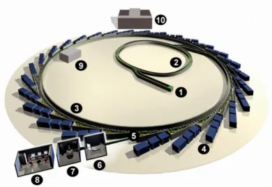
2.15 Schematic of the Diamond Light Source site. 42
2.16 Insertion device consisting of alternately-arranged magnets causing the electron
beam to oscillate. 45
2.17 Schematic of beamline I11 at Diamond. 45
2.18 Diffractometer with Bragg-Brentano geometry. 46
2.19 Schematic of a powder diffractometer. 48
2.22 A graphical method for indexing the cubic system. 55
2.23 Lorentz Polarisation factor profile. 71
2.24 Full profile refinement of an XRPD pattern using the program GSAS. 74
3.1 DSC schematic. 77
3.2 Netzsch ST449 F3 Jupiter DSC. 78
3.3 Sample carrier with reference and sample pans atop. 79
3.4 Cut-away schematic of the DSC. 80
3.5 DSC curve showing heat flow against temperature (exothermic is ‘up’). 81
3.6 20K/min ramp for praseodymium oxide. 84
4.1 Changes in peak intensity over time. 87
4.2 Sigmoidal function (top) and its linearised form. 93
4.3 Germ nucleation, grain growth and grain impingement. 94
4.4 Illustration of extended volume. 95
5.1 Raw data (intensity versus 2θ) displayed in PowderX. 102
5.2 Histogram after removal of Kα2 contribution and background, and identification of
peak positions. 103
5.3 Crysfire peak position input screen. 104
5.4 Summary file of indexing results. 105
5.5 CHEKCELL main screen showing trial cells (top half) and comparison of measured
and calculated peak positions (bottom half). 106
5.6 Best solution from CHEKCELL. 107
5.7 Unit cell refinement in CHEKCELL (mean square deviation for the refined
parameters is lower than initial parameters). 107
5.8 Histogram after refinement in GSAS. 109
5.9 Combined DSG-TG plot. 110
7.1 XRPD pattern for sample (1) Eu2O3. 117
7.2 XRPD pattern for sample (1) Eu2O3 showing the region between 46° and 64° in
more detail. 117
7.3 XRPD pattern for sample (2) Gd2O3. 118
7.6 XRPD pattern for sample (3) Yb2O3 showing the region between 46° and 64° in
more detail. 119
7.7 XRPD pattern for sample (4) Pr2O3. 120
7.8 XRPD pattern for sample (4) Pr2O3 showing the region between 46° and 64° in
more detail. 120
7.9 XRPD pattern for sample (5) Tb2O3. 121
7.10 XRPD pattern for sample (5) Tb2O3 showing the region between 46° and 64° in
more detail. 121
7.11 XRPD pattern for sample (9) Nd2O3. 122
7.12 XRPD pattern for sample (10) Sm2O3. 122
7.13 XRPD pattern for sample (11) Eu2O3. 123
7.14 Plot of cell parameter against atomic number for the C-type cell. 124
7.15 Crystal structure of the C-type cubic phase in space group Ia-3. 125
7.16 Crystal structure of the B-type monoclinc phase in space group C2/m. 127
7.17 Crystal structure of the A-type hexagonal phase in space group P-3m1. 128
7.18 XRPD pattern for sample (1) Eu2O3 following 1 hour anneal at 1334ºC and slow
cooling. 131
7.19 XRPD pattern for sample (2) Gd2O3 following 1 hour anneal at 1334ºC and slow
cooling. 131
7.20 XRPD pattern for sample (2) Gd2O3 following 1 hour anneal at 1500ºC and
quenching. 132
7.21 XRPD pattern for sample (2) Gd2O3 following 7 hour anneal at 1500ºC and
quenching. 132
7.22 XRPD pattern for sample (2) Gd2O3 following 7 hour anneal at 1500ºC and
quenching showing the region between 28° and 35° in more detail. 133
7.23 XRPD pattern for sample (3) Yb2O3 following 1 hour anneal at 1500ºC and
quenching. 133
7.24 XRPD pattern for sample (3) Yb2O3 following 5 hour anneal at 1500ºC and
quenching. 134
7.25 XRPD pattern for sample (7) Yb2O3 following 5 hour anneal at 1800ºC and
quenching. 134
7.27 XRPD pattern for sample (8) Gd2O3 following 7 hour anneal at 1500ºC and
quenching showing the region between 14° and 18° in more detail. 135
7.28 Plot of cell parameter against atomic number for the B-type cell. 137
7.29 Diffraction pattern of Gd2O3 following 1 hour anneal at 1334ºC showing
low-intensity reflections due to the monoclinic phase. 140
7.30 Diffraction pattern of Gd2O3 following 1 hour anneal at 1500ºC showing
low-intensity reflections due to the monoclinic phase. 141
7.31 Cubic (upper image) and monoclinic (following 7 hour anneal at 1500ºC) patterns
for Gd2O3. 142
7.32 Estimation of unit cell parameter ‘a’ for monoclinic Gd2O3 by a method of
interpolation. 143
7.33 XRPD pattern of Yb2O3 post-heating to 1500ºC showing low-intensity reflections
due to the monoclinic phase. 145
7.34 Praseodymia ramp 25ºC to 275ºC showing the appearance of the ceria-type
β
phase (Pr6O11) at 275ºC. 147
7.35 Praseodymia ramp 300ºC to 550ºC showing the ceria cell throughout. 148
7.36 Praseosymia ramp 575ºC to 800ºC showing the appearance of the
ι
phase(Pr7O12) at 625ºC. 149
7.37 Final stage of refinement of the
β
phase (Pr6O11) of praseodymia. 1507.38 Final stage of refinement of the
ι
phase (Pr7O12) of praseodymia. 1507.39 Praseodymia ramp 800ºC to 450ºC showing the loss of the
ι
phase of Pr7O12 at575ºC. 151
7.40 Praseodymia ramp 425ºC to 125ºC showing the ceria cell throughout. 152
7.41 The five Bragg peaks of the
β
phase emerging from the ambient mixed phaseduring the 250°C isothermal hold. 153
7.42 Conversion against time for Pr2O3 to Pr6O11 phase change using the increase in
intensity of the 47.2º (
β
phase 220 plane) peak. 1547.43 Shrinking Sphere kinetic isotherms for the 47.2º (
β
phase 220 plane) peak. 1557.44 Plot of ln k against 1/T for the 47.2º (
β
phase 220 plane) peak. 1568.1 DSC-TG recorded on sample (4) Pr2O3 from 20°C to 1550°C at 10K/min under
nitrogen. 162
8.2 DSC-TG recorded on sample (4) Pr2O3 from 20°C to 1550°C at 10K/min under
nitrogen. 2nd attempt. 163
8.3 DSC-TG recorded on sample (4) Pr2O3 from 20°C to 1550°C at 10K/min under
nitrogen following heating at 170°C for 10 minutes. 165
8.4 DSC 4 recorded on sample (4) Pr2O3 from 20°C to 1550°C at 10K/min under
nitrogen following heating at 380°C for 10 minutes. 165
8.5 Mettler DSC-TG recorded on sample (4) Pr2O3 from 20°C to 1100°C 167
8.6 DSC-TG recorded on sample (6) from 20°C to 1500°C at 10K/min under air. 168
8.7 DSC recorded on sample (4) Pr2O3 from 200°C to 500°C under nitrogen. 169
8.8 Temperature of maximum deflection, Tm, versus heating rate,
φ
, for sample 1708.9 Plot of ln (
φ
/Tm2) against 1/Tm for sample (4) Pr2O3 1st endotherm. 1718.10 Temperature of maximum deflection, Tm, versus heating rate,
φ
, for sample (4)Pr2O3 2nd endotherm. 172
8.11 Plot of ln (
φ
/Tm2) against 1/Tmfor sample (4) Pr2O3 2nd endotherm. 1728.12 Temperature of maximum deflection, Tm, versus heating rate,
φ
, for sample (4)Pr2O3 3rd endotherm. 173
8.13 Plot of ln (
φ
/Tm2) against 1/Tm for sample (4) Pr2O3 3rd endotherm. 1748.14 DSC ramps on sample (6) Pr2O3 from 200°C to 600°C in air. 175
8.15 Temperature of maximum deflection, Tm, versus heating rate,
φ
, for sample (6)Pr2O3 1st exotherm. 176
8.16 Plot of ln (
φ
/Tm2) against 1/Tm, for sample (6) Pr2O3 1st exotherm. 1768.17 DSC ramps on sample (6) Pr2O3 from 20°C to 1500°C in air. 177
8.18 Temperature of maximum deflection, Tm, versus heating rate,
φ
, for sample (6)Pr2O3 1st exotherm. 178
8.19 Plot of ln (
φ
/Tm2) against 1/Tm for sample (6) Pr2O3 1st exotherm. 1798.20 Temperature of maximum deflection, Tm, versus heating rate,
φ
, for sample (6)1250°C endotherm. 180
8.22 DSC recorded on sample (6) Pr2O3 from 20°C to 1400°C and back at 10K/min in
air. The data collected from 20°C to 1500°C (from figure 8.6) is shown on the left for
comparison. 182
8.23 DSC-TG recorded on sample (6) Pr2O3 from 20°C to 1400°C and back at 10K/min
in air. 183
8.24 DSC-TG recorded on sample (6) Pr2O3 from 20°C to 1400°C and back at 10K/min
in air. Image wrapped to compare associated transitions. 184
8.25 DSC-TG recorded on sample (6) Pr2O3 from 20°C to 1400°C and back at 10K/min
in air. Mass changes are shown. 184
8.26. Gas loss from sample (6) Pr2O3 after 85 days’ exposure to air. 186
8.27 DSC-TG recorded on sample (6) Pr2O3 from 20°C to 1500°C at 10K/min in air.
Mass changes are indicated. 188
8.28 Temperature versus oxygen in the Pr-O system for DSC recorded on sample (6)
Pr2O3 at 10K/min in air. 189
8.29 Temperature versus oygen content for all DSC recorded on sample (6) Pr2O3 from
20°C to 1500°C in air. 190
8.30 DSC recorded on sample (6) Pr2O3 at 2K/min in air with phases marked. 192
8.31 Phases attained during ramps on sample (6) Pr2O3. 193
8.32 Hysteresis loop for the
α
phase toι
phase (Pr7O12) transition. 1958.33 Temperature-composition plot for the
ι
-σ
-θ
region. 1968.34 Isobaric runs on Pr2O3. 198
9.1 Amended phase diagram for the lanthanoid sesquioxides. 207
9.2. Amended phase diagram for the praseodymium-oxygen system showing the
σ
LIST OF TABLES
1.1 Electron configurations of the lanthanoid atoms and their tripositive ions. 4
1.2 Electron configurations of the lanthanoids. 6
1.3 Unit cell parameters for the cubic series Rb2NaLnF6 (ICDD 1995). 9
1.4 Unit cell parameters for the tetragonal series LiLnF4 (ICDD 1995). 10
1.5 Discrete phases in the praseodymium-oxygen system. 17
2.1 The seven crystal systems. 25
2.2 Values of h, k and l for cubic lattices. 30
2.3 X-ray wavelengths for typical anode metals. All values in Angströms. 41
2.4 Arithmetic derivation of unit cell parameter for a cubic cell. 57
2.5 Arithmetic method for indexing the cubic system. 58
2.6 Arithmetic method for indexing the tetragonal system. 60
2.7 Values of Qhkl expressed using reciprocal cell parameters. 66
4.1 Values of the Avrami exponent and corresponding geometries. 97
6.1 Samples obtained for XRPD and DSC-TG. 111
6.2 XRPD schedule for samples. 112
6.3 Heating scheme for samples. 112
6.4 XRPD schedule for annealed samples. 113
6.5 Pre-DSC-TG heating schedule for sample (4). 114
7.1 Refined unit cell parameters for samples (1) to (5) and (9) to (11). 123
7.2 Crystal structure of cubic Pr2O3. 125
7.3 Crystal structure of cubic Eu2O3. 125
7.4 Crystal structure of cubic Eu2O3. 126
7.5 Crystal structure of cubic Gd2O3. 126
7.6 Crystal structure of cubic Tb2O3. 126
7.7 Crystal structure of cubic Yb2O3. 126
7.8 Crystal structure of monoclinic Sm2O3. 127
7.9 Crystal structure of hexagonal Pr2O3. 128
7.10 Crystal structure of hexagonal Nd2O3. 128
7.12 Crystal structure of monoclinic Eu2O3. 138
7.13 Crystal structure of monoclinic Gd2O3. 138
7.14 Crystal structure of monoclinic Gd2O3 from synchrotron data. 138
7.15 Crystal structure of Pr6O11. 139
7.16 Crystal structure of Pr7O12. 139
7.17 Values of the rate constant, k, for the 47.2º (
β
phase 220 plane) peak. 1557.18 Values of the rate constant and Avrami exponent for the 47.2º (
β
phase 220 plane)peak. 157
7.19 Values for activation energy. 159
7.20 Activation energies for the lanthanide oxides. 161
8.1 Kissinger analysis for 1st endotherm - sample (4) Pr2O3. 170
8.2 Kissinger analysis for 2nd endotherm - sample (4) Pr2O3. 171
8.3 Kissinger analysis for 3rd endotherm - sample (4) Pr2O3. 173
8.4 Kissinger analysis for 1st exotherm - sample (6) Pr2O3. Data recorded from 200°C
to 600°C. 175
8.5 Kissinger analysis for 1st exotherm - sample (6) Pr2O3, Data recorded from 20°C to
1500°C. 178
8.6 Kissinger analysis for endotherm at 1250°C - sample (6) Pr2O3. Data recorded from
20°C to 1500°C. 179
8.7 Activation energies for phase changes in samples (4) and (6). 181
8.8 Transition temperatures for sample (6) Pr2O3 taken from 10K/min DSC-TG data.
185
8.9 Weight loss on sample (6) Pr2O3 on exposing to air. 186
8.10 Values of x in PrOx for DSC-TG recorded on sample (6). 190
8.11 Order of appearance of phases in the Pr-O system with temperature for the 2K/min
ramp. 191
8.12 Kinetic data for the Pr-O system. 199
9.1 Comparison of activation energy data from XRPD and DSC. 205
9.2 Activation energies for the lanthanide oxides. 205
ACKNOWLEDGEMENTS
Thanks are due to my academic supervisors Professor Susan H. Kilcoyne and Professor Neil M. Boag, who provided advice and support through the course of my work.
Additional thanks are due to:
Geoff Parr of Salford Analytical Services for running samples on the Siemens D500
and Bruker D8 X-ray powder diffractometers and for his technical advice;
Peter Skingle of Manchester Metropolitan University for access to the Heraeus furnace;
Dr Tim Comyn of Leeds University for access to the Philips PANalytical X’Pert
powder diffractometer;
Dr Wei Loh and Zhenggang Lian of Southampton University for access to the 1800°C
glass furnace;
Professor Chiu Tang, Principal Beamline Scientist on Beamline I11 at Diamond Light
Source, for obtaining XRPD data;
Phil Williams of Mettler Toledo for obtaining additional DSC data;
DECLARATION
The research in this thesis is my own work with the following exceptions.
All XRPD data collected on the Siemens and Bruker machines were performed by
Geoff Parr of Salford Analytical Services.
Sample (7) of Yb2O3 was annealed by Zhenggang Lian of Southampton University.
The XRPD pattern obtained at Diamond Light Source was collected on beamline I11
by Professor Chiu Tang.
The DSC data represented in figure 8.5 was collected by Phil Williams of Mettler
ABSTRACT
The lanthanoid sesquioxides exhibit a number of distinct structural phases. Below
2000°C these oxides exist in three crystal systems, namely the A-type hexagonal phase,
the B-type monoclinic phase and the C-type cubic phase. With increasing temperature
the stability of these structures is generalised by the order C → B → A, although not
every oxide will exhibit all phases; this general transition is typical of the middle
members of the group. Under ambient conditions, the A phase is preferred for La2O3 to
Pm2O3. Both the C and B phases exist for Sm2O3, Eu2O3 and Gd2O3. The C phase is
stable at room temperature from Sm2O3 onwards, and at the high atomic number end of
the series this phase is preferred.
Traditionally, the structures of the heavier sesquioxides (Er2O3 to Lu2O3) have been
believed to be cubic from ambient temperature all the way up to their melting points.
However, contrary to the current phase diagram, my work has shown that not only are
B-type Sm2O3, Eu2O3 and Gd2O3 very stable at ambient temperature, but it is also
possible to create 1% monoclinic Yb2O3 by heating and then quenching back to
ambient temperature.
Of the lanthanoids, praseodymium and terbium are known for their existence in both
the +3 and +4 oxidation states. The praseodymium-oxygen system is notable for its
multiple stoichiometries. This work presents kinetic data for the
φ
→β
phase and theσ
→
θ
phase transitions in this system, the results obtained via high-temperature X-raypowder diffraction and differential scanning calorimetry.
The crystal structures of B-type Gd2O3 and Yb2O3 are reported, the former obtained
using both laboratory and synchrotron X-ray data and the latter using laboratory data
alone. It is proposed that this is the first time these two structures have been determined
following the application of temperature alone, without the additional application of
DEDICATION
For Phyllis Margaret Skinner
1 INTRODUCTION
1.1THE RARE EARTHS
The rare earths constitute a series of highly electropositive elements occupying period 6
of the periodic table between the 6s and 5d blocks and their occurrence marks the first
occupying of the 4f atomic orbitals in the ground state. Unlike the d block elements
their chemistry is fairly uniform across the series, with the +3 oxidation state
dominating.
The series corresponds to the filling of the 4f atomic orbitals from lanthanum, which
has an electronic configuration [Xe]5d16s2, to lutetium, [Xe]4f145d16s2. As the
members of the series have similar properties they are referred to in the IUPAC scheme
as the lanthanoids, after the first element in the series, lanthanum, which itself takes its
name from the Greek λανθανειν (lanthanein), meaning to lie hidden. Despite this, the
term lanthanides is still widely in use. All the lanthanoids have similar chemical
properties, since the 4f atomic orbitals are of a smaller radial extension than the 6s and
5d atomic orbitals in which the valence electrons lie and hence do not greatly affect the
chemistry of the elements. The f orbitals are said to be buried inside the atom and
shielded from its external environment by the valence electrons. This means that the
chemistry of the lanthanoids is largely determined by their atomic radii.
All the lanthanoids show the +3 oxidation state. An unusual deviation from this is seen
with cerium, which can exhibit the +4 state, achieving the electronic stability of the
noble gas xenon. Europium exhibits the +2 state, achieving the stability of a half-filled
f shell. The +4 oxidation state is also seen with praseodymium and terbium. The
element promethium does not occur in nature.
Although not actually lanthanoids, yttrium and scandium are often considered to be rare
earths as they occur in the same sources. Yttrium, [Kr]4d15s2, is the immediate vertical
neighbour of lanthanum, has a similar electronic configuration and shows a great
elements more strongly than it does any of the other lanthanoids. Scandium, [Ar]3d14s2,
the lightest member of the transition elements and again vertical to lanthanum, also
resembles the lanthanoids closely in its chemical properties.
The term rare earths is actually a misnomer. Cerium is the twenty-fifth most abundant
element in the earth and is as common as copper. Even the least-common rare earth,
thulium, occurs in greater proportion than mercury. However, because the rare earths
have a similar chemistry and tend to occur naturally together, historically their
separation from each other has been difficult. It is this fact that has given the
impression of their rarity. The phrase to lie hidden indicates that the metals are difficult
to separate i.e. they lie hidden behind each other. Originally, separation was performed
by a laborious series of fractional crystallisations. As the lanthanoid ions have subtly
different radii, the lattice energies of their salts and their hydration energies are also
different. This means that they have slight differences in solubility and hence different
metal salts will precipitate from solution at slightly different concentrations. In recent
times, separation of ions has been achieved by solvent extraction and ion exchange.
Both methods rely on the small differences in ionic radii across the group.
Typical sources of rare earths are monazite sand, the mineral xenotime (which both
contain a mixture of the phosphates of lanthanoids and thorium) and bastnaesite (which
contains lanthanoid fluorocarbonates). In terms of their occurrence in the earth’s crust,
lanthanum, cerium and neodymium are by far the most common. The rare earths have
many applications. Their most common use is in catalytic converters for internal
combustion engines. They also have use as refining catalysts in the petrochemical
industry. Other uses include alloying material in permanent magnets, colours for glass
and ceramics, phosphors, and doping agents for lasers. Cerium is contained in the alloy
known as misch metal, used as the flint of cigarette lighters. It is also used as an
anti-knock agent in petrol. Europium is used within nuclear fuel control rods and also within
the red phosphor in CRT television screens. Ytterbium has been shown to have an
1.2 THE STABILITY OF THE TRIPOSITIVE OXIDATION STATE
The ground state electronic configurations of the uncharged lanthanoid atoms and their
tripositive ions are given in table 1.1. For the atoms, the 4f orbitals are generally more
stable than the 5d, illustrated by the fact that the 5d orbitals are only occupied in a few
cases. After lanthanum the 5d orbitals are empty and only when gadolinium is reached
is the extra stability of the half-filled 4f orbitals sufficient to induce reoccupation of the
5d orbitals. For the tripositive ions, chemically the most important oxidation state, the
4f orbitals are much more stable and the 5d and 6s orbitals are not occupied at all. The
electron configurations of the tripositive ions reveal a sequential filling of the 4f atomic
orbitals from lanthanum at f0 to lutetium at f14.
The 4f electrons occupy space inside the n = 5 shell. They are more stable and have
greater ionisation potentials than the 5d and 6s electrons. Consequently the loss of the
6s and 5d electrons is always seen before that of the 4f electrons. This is illustrated by
electronic absorption spectra of compounds of tripositive lanthanoid ions. As a general
trend, ionisation energy increases with atomic number and shows marked half-shell
effects. Table 1.1 lists both the sum of the first three ionisation potentials and the fourth
Z Element Electron config.
Electron config. for Ln3+
Ionic radius (pm) 6CN†
ΣIP1-3 *
kJ.mol-1 IP4
**
kJ.mol-1
[image:23.595.100.499.73.378.2]57 La [Xe]5d16s2 f0 117.2 3455 4819 58 Ce [Xe]4f15d16s2 f1 115 3523 3547 59 Pr [Xe]4f36s2 f2 113 3627 3761 60 Nd [Xe]4f46s2 f3 112.3 3697 3899 61 Pm [Xe]4f56s2 f4 111 3740 3966 62 Sm [Xe]4f66s2 f5 109.8 3869 3994 63 Eu [Xe]4f76s2 f6 108.7 4036 4110 64 Gd [Xe]4f75d16s2 f7 107.8 3749 4245 65 Tb [Xe]4f96s2 f8 106.3 3791 3839 66 Dy [Xe]4f106s2 f9 105.2 3911 4001 67 Ho [Xe]4f116s2 f10 104.1 3924 4101 68 Er [Xe]4f126s2 f11 103 3934 4115 69 Tm [Xe]4f136s2 f12 102 4045 4119 70 Yb [Xe]4f146s2 f13 100.8 4194 4220 71 Lu [Xe]4f145d16s2 f14 100.1 3887 4360
Table 1.1 Electron configurations of the lanthanoid atoms and their tripositive ions.
†
metal cation showing six-fold coordination (Shannon 1976)
As a generalisation, IP4~2(IP3)~4(IP2)~8(IP1) and IP4 > (IP1+IP2+IP3)
*
sum of first three ionisation potentials (Bernal et al 2004)
**
fourth ionisation potential (Bernal et al 2004)
Figure 1.1
Σ
IP1-3 and IP4 for the lanthanoids (Bernal et al 2004).Table 1.1 shows that the sum of the first three ionisation potentials for the lanthanoids
is fairly consistent across the series, indicating the +3 state to be a common one.
Indeed, this state is the preferred one under ambient conditions for most elements in the
series, other than those with a relatively low second or fourth ionisation potential.
Cerium, praseodymium and terbium all exhibit the +4 state, as well as displaying
oxides with mixed +3/+4 valencies such as Pr6O11 and Tb4O7. Cerium is the only
lanthanoid to be stable in the +4 oxidation state in aqueous solution. The only binary
cerium IV compounds known are CeF4 and CeO2. There are several stable complexes
containing Ce4+, for example (NH4)2[Ce(NO3)6], in which the nitrate ion acts as a
bidentate ligand, the co-ordination of the Ce4+ being icosahedral. Only europium
shows a marked tendency for lower oxidation states, for example Eu2+ exists in EuO
and EuC2O4, although neodymium, samarium and ytterbium also show some tendency
for this oxidation state. Table 1.2 below lists the oxidation states attainable by the
Element Oxidation state Electron configuration
La +3 [Xe] noble gas
Ce +3
+4
[Xe]4f1 [Xe] noble gas
Pr +3 +4 [Xe]4f2 [Xe]4f1 Nd +2 +3 [Xe]4f4 [Xe]4f3
Pm +3 [Xe]4f4
Sm +2 +3 [Xe]4f6 [Xe]4f5 Eu +2 +3
[Xe]4f7 half shell [Xe]4f6
Gd +3 [Xe]4f7 half shell
Tb +3
+4
[Xe]4f8
[Xe]4f7 half shell
Dy +3 [Xe]4f9
Ho +3 [Xe]4f10
Er +3 [Xe]4f11
Tm +3 [Xe]4f12
Yb +2
+3
[Xe]4f14 full shell [Xe]4f13
[image:25.595.192.441.73.483.2]Lu +3 [Xe]4f14 full shell
Table 1.2 Electron configurations of the lanthanoids.
1.3 THE LANTHANIDE CONTRACTION
The elements in the first row of the f block exhibit a decrease in atomic radius from
lanthanum, Z=57 to lutetium, Z=71. Because of this phenomenon, termed the
lanthanide contraction, vertically-adjacent elements in the 2nd and 3rd rows of the d
block, which appear before and after the lanthanoids, have very similar atomic radii
even though they contain very different numbers of electrons. For example, the atomic
row of the f block there is a steady decrease in atomic radius with increasing atomic
number. This contraction is also shown in the radii of the tripositive ions, illustrated in
figure 1.2. This decrease in ion size is accompanied by the filling of the 4f orbitals.
Before the electronic structures of the lanthanoids were elucidated by spectroscopy,
they could only be assumed. It was correctly believed that the electronic structure of the
lanthanum atom was [Xe]5d16s2. It was therefore easy to explain the existence of the
+3 oxidation state by the loss of the three outer electrons. Assuming that the 5d16s2
electrons were retained across the series of atoms from [Xe]5d16s2 to [Xe]4f145d16s2
and that moving across the lanthanoids corresponded to the filling of the 4f shell, the
predominance of the +3 oxidation state could be explained as each atom could lose the
5d16s2 electrons to form the tripositive ion. However, spectroscopy has revealed that the
atoms and ions do not all have the [Xe]4fn5d16s2 and [Xe]4fn structures respectively.
The removal of electrons from a lanthanoid atom proceeds in the manner of first the
outer 6s electrons, secondly the outer 5d electrons and thirdly the 4f electrons. Because
of their greater affinity for the nucleus and hence the shorter radial extension of their
atomic orbitals, the 4f electrons are termed inner or core electrons.
In a multi-electron atom, the distance an electron exists from the nucleus is determined
by both the shell in which it lies and the nuclear charge. Increasing nuclear charge
causes a shrinking of the atomic radius. However, this shrinkage is offset to some
degree by the presence of the inner electrons. This is due to a shielding effect; inner
electrons shield the outer electrons from the nucleus. Therefore, rather than experience
the full nuclear charge, Z, the outer electrons experience an effective nuclear charge,
Zeff. The shielding effect of occupied atomic orbitals decreases in the order s > p > d >
f. Because of their limited radial extension and their highly angular shapes, the 4f
atomic orbitals have a poor shielding effect and the shielding gained on adding
electrons to the 4f orbitals on crossing the lanthanoid series fails to compensate for the
increasing nuclear charge. For the lanthanoids, Zeff is seen to increase steadily with
increasing atomic number, causing the electrons to be drawn in towards the nucleus.
Consequently there is a steady and almost linear decrease in atomic radius with
Figure 1.2 Ionic radii for the tripositive ions Z=57 to 71 (Shannon 1999).
This poor shielding ability of the 4f electrons is believed to be the major contributor to
the lanthanide contraction, although studies reveal about 10% of the contraction is due
to relativistic effects (Pyykkö and Descleaux 1979). In heavy atoms such as the
lanthanoids, the effects of special relativity become significant for high-speed electrons
and result in both a contraction of the radial extension of atomic orbitals and an
increase in the rest mass of electrons. Consequently there is a decrease in the atomic
radius. Other notable examples of chemical relativistic effects are the physical state of
mercury at ambient temperature and the colour of gold. Mercury is known to exist as
the monoatomic species Hg in the gaseous state. The contraction of the valence
electron shell means it does not play a significant role in bonding and so the atoms in
the liquid are held together by weak Van der Waals forces alone. With gold, the
contraction of the 6s orbital means the 5d → 6s energy transition is shifted from the
ultra-violet into the visible part of the electromagnetic spectrum. The wavelength of
light concerned is in the blue region of the spectrum, resulting in the metal having its
1.3.1 The lanthanide contraction illustrated in unit cell parameters
Because of the existence of the lanthanide contraction the possibility arises that the unit
cell parameters for particular series of compounds might also follow a contraction. For
example, if a particular lanthanoid compound exhibits cubic symmetry, then the rest of
the lanthanoids when present in the same type of compound might also exhibit the
same symmetry. Furthermore, a plot of the unit cell parameter against atomic number
might show a trend similar to that of the lanthanide contraction. There are many
references citing cases of series of lanthanoid compounds exhibiting a common
structure (Siddiqui and Hoppe 1975), (Feldner and Hoppe 1980), (Urland et al 1980),
(Aléone and Pouzet 1968). Aléone and Pouzet consider the series of compounds
Rb2NaLnF6 and Cs2NaLnF6, where Ln is a lanthanoid, and state that all are cubic with
the perovskite structure and of space group Fm3m. Unit cell data for the series of cubic
structures Rb2NaLnF6 is given in table 1.3 and illustrated in figure 1.3. It is clear that
the trend in the cell size across the series is similar to that of the tripositive ionic radii.
Data for the series of tetragonal structures LiLnF4 is given in table 1.4 and illustrated in
figure 1.4. ICDD is the International Centre for Diffraction Data.
Z Element ICDD ref Cell a (Å) Crystal
system
Space group
62 Sm 21-1041 8.988 Cubic Fm3m 65 Tb 21-1042 8.921 Cubic Fm3m 67 Ho 21-1040 8.881 Cubic Fm3m 68 Er 20-1384 8.867 Cubic Fm3m 70 Yb 21-1043 8.816 Cubic Fm3m
Figure 1.3 Atomic number versus unit cell parameter for the cubic series Rb2NaLnF6
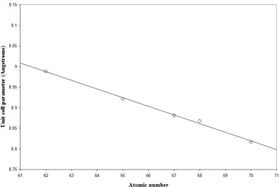
(ICDD 1995).
Z Element ICDD ref Cell a (Å) Cell c (Å) Crystal
System
Space group
[image:29.595.119.514.70.335.2]63 Eu 27-0292 5.21 11.02 Tetragonal I41/a 64 Gd 27-1236 5.21 11.00 Tetragonal I41/a 65 Tb 27-1262 5.19 10.89 Tetragonal I41/a 66 Dy 27-1233 5.19 10.81 Tetragonal I41/a 67 Ho 27-1243 5.16 10.75 Tetragonal I41/a 68 Er 27-1235 5.16 10.70 Tetragonal I41/a 69 Tm 27-1265 5.15 10.64 Tetragonal I41/a 70 Yb 23-0371 5.13 10.58 Tetragonal I41/a 71 Lu 27-1251 5.13 10.53 Tetragonal I41/a
Figure 1.4 Atomic number versus unit cell parameters for the tetragonal series LiLnF4
(ICDD 1995).
Because of this trend across series of lanthanoid compounds, it is often a good starting
point when considering an unknown structure to look at the structures of the same
compounds of the adjacent metals. In many cases the cell type and space group will be
the same. Furthermore, the unit cell parameters may be the same, subject to an
adjustment according to the lanthanide contraction. In such a case, the atom positions
are also likely to be the same. However, a single cell type is not generally
representative of any one series of lanthanoids. There are series of compounds where
the shrinking co-ordination sphere of the metal induces a change in cell type. For
example, with the lanthanoid sesquioxides there is a shift from the 7-fold co-ordination
of a hexagonal structure, to the 6-fold co-ordination of a cubic structure. In such a
series a break would be seen in the plot of unit cell parameters; a pair of lines
corresponding to the values for a and c in the hexagonal cell would switch to a single
line corresponding to the single cubic cell parameter. For both cell types the plots
1.4 LANTHANOID COMPOUNDS
1.4.1 Overview
The crystal structure of the simple compounds such as the sesquioxides and halides
exhibit high co-ordination numbers due to the large sizes of the tripositive lanthanoid
ions. The sesquioxides are the most stable oxides, except for those of cerium,
praseodymium and terbium, whose oxides contain the metal wholly (cerium) or partly
(praseodymium and terbium) in the +4 oxidation state. At ambient temperature the
sesquioxides of the lighter lanthanoids exhibit hexagonal symmetry. Heavier
sesquioxides exhibit cubic symmetry. The monoxide of europium is known but there is
doubt as to the phases of other low-oxygen species. Higher oxides exist, notably that of
cerium. Ceric oxide, CeO2, has the fluorite structure (as do PrO2 and TbO2) but a range
of phases is known to exist, with some intermediate between Ce2O3 and CeO2, for
example Ce32O58, Ce32O57 and Ce18O31. The compound Pr6O11 exists as a mixed phase
of the +3 and +4 oxides in the ratio 1:4 and may be converted to Pr2O3 with hydrogen
at high temperature. As with cerium there exists a range of phases between the
sesquioxide and the dioxide. The intermediate oxide Ln7O12 is also known for
lanthanum, cerium, praseodymium and terbium. The general property of many rare
earth oxides is that they have defect lattices in which some O2- vacancies in the LnO2
fluorite structure are compensated for by the presence of Ln3+ ions.
The sulphides, selenides and tellurides exhibit the compounds LnS, Ln3S4, Ln2S3 and
LnS2 but there are many non-stoichiometric compounds in addition to these. The
interest in these compounds lies in their semi-conducting properties.
The hydroxide ion has a similar radius to the fluoride ion and consequently, for the
light lanthanoid trifluorides and hydroxides, the same crystal structure is exhibited, that
of tysonite, LnF3, with each lanthanoid co-ordinated to 9 fluorides anions. For the
The tribromides adopt the same structures as the trichlorides. The triiodides adopt the
PuBr3 structure for lanthanum to neodymium and the FeCl3 structure for samarium to
lutetium. Lower halides are known; the difluorides of samarium, europium and
ytterbium exhibit the fluorite structure. The difluorides of thulium and ytterbium
exhibit the structure of CaI2. The dichlorides of neodymium, samarium, europium,
dysprosium and ytterbium are prepared by the reduction of the trichloride with the
lanthanoid. The dibromides of samarium, europium, thulium and ytterbium and the
diiodides of lanthanum, cerium, praseodymium, neodymium and gadolinium are
prepared in a similar way. Diiodides are also obtained by thermal decomposition of the
triodides. Tetrafluorides of cerium, praseodymium and terbium are known, having the
UF4 structure of a square anti-prism. Attempts to make other tetrafluorides have been
unsuccessful but the complexes Cs3[NdF7] and Cs3[DyF7] have been made by
fluorination of a mixture of caesium chloride and the lanthanoid trichloride. As a
general rule, for all classes of compounds there is a trend of decreasing co-ordination
number with decreasing ionic radius.
1.4.2 The lanthanoid sesquioxides
Historically the lanthanoid sesquioxides have been extensively studied, the first notable
publication being in 1925 (Goldschmidt et al 1925). This study first highlighted the
three structural types, A, B and C. Their crystallographic forms and polymorphism
have been reviewed on a number of occasions (Brauer 1968), (Haire and Eyring 1994),
(Adachi and Imanaka 1998), (Zinkevich 2007). Below 2000°C the sesquioxides exist in
three crystal systems i.e. the cubic C-type, the monoclinic B-type and the hexagonal
A-type. With increasing temperature the stability of the structures is generalised by the
order C → B → A, although not every oxide will exhibit all phases; this general
transition is typical of the middle members of the group. Under ambient conditions the
A-type oxide is preferred for lanthanum to promethium, although it may exist in
combination with the C-type. C-type cerium sesquioxide is actually a
non-stoichiometric oxide showing a range of oxygen content, but designated Ce2O3. Both C
and B-type oxides exist for samarium, europium and gadolinium. The C-type is stable
oxide, the fraction of B-type falling with increasing weight of the metal. For lutetium
the C-type oxide is the only phase known, as there is a direct transition to the molten
state at approximately 2400°C.
Above 2000°C an additional two types, denoted by H and X, are present (Föex and
Traverse 1966). These are believed to be modifications of the hexagonal and cubic
phases, respectively (Aldebert and Traverse 1979). Only a very few lanthanoid
sesquioxides exhibit all five phases (promethium, samarium and europium). A phase
diagram showing all five modifications is given in figure 1.5.
Figure 1.5 Phase diagram for the lanthanoid sesquioxides (Föex and Traverse 1966).
and X-types are reached at over 2000°C. For the intermediate oxides, the ambient phase
is cubic. On heating, there is a transition to the monoclinic phase before the H and
X-types are reached. After holmium sesquioxide, the only phase is cubic until the H phase
is reached.
The structures of the three main phases are well known. The A-type exists in space
group P-3m1 with one formula unit per unit cell. The metal atoms occupy the 4f sites of
the space group. 4 of the oxygen atoms occupy the same sites; the remaining 2 oxygen
atoms occupy the 2a sites. The metal atoms are in seven-fold co-ordination to oxygen
with four oxygen atoms closer than the other three.
Figure 1.6 A-type (hexagonal) Ln2O3 (where Ln represents any lanthanoid). Solid dots
represent metal centres (Eyring 1979).
The B phase, a distortion of the A-type, exists in space group C2/m with six formula
units per unit cell. All 12 metal atoms occupy the 4i sites of this space group. 16
oxygen atoms also occupy the 4i sites, with a further 2 oxygens occupying the 2b sites.
Figure 1.7 B-type (monoclinic) Ln2O(Eyring 1979).
The C-type has the bixbyite structure in space group Ia-3, bixbyite having its most
common form as Mn2O3. The unit cell contains 32 metal atoms (on the 8b and 24d
sites) and 48 oxygen atoms (occupying all 48e sites). The structure is effectively a
fluorite lattice with a quarter of the oxygen sites vacant. In this structure the metal
atoms are six-fold co-ordinated to oxygen.
1.4.3 The praseodymium-oxygen system
When the ratio of oxygen to metal is variable, the praseodymium-oxygen system shows
a number of discrete phases. In fact, of all the rare earth oxides, the
praseodymium-oxygen system is the most complex. In addition to the green-coloured sesquioxide there
are six well-established and well-studied oxides. The majority of work on the
praseodymium-oxygen system comes from Eyring and co-workers in a series of papers,
the most significant of which (Hyde et al 1965) established the phase diagram in figure
1.9. Here is confirmed the existence of the
ι
(x = 1.71),ξ
(x = 1.78),ε
(x = 1.80) andβ
(x = 1.83) phases, together with two wide-ranging non-stoichiometric phases. These are
the face-centred
α
phase, with 2.00 ≥x≥ 1.72 and the body-centredσ
phase, with 1.7 ≥x ≥ 1.6. Observed for the first time is the
δ
(x = 1.816) phase. It was also establishedthat the discrete monophasic species were members of an incomplete homologous
series corresponding to the formula PrnO2n-2 for values of n = 4, 7, 9, 10, 11, 12 and ∞.
These phases are listed in table 1.5.
n Formula phase x in PrOx Cell Existence 4 Pr2O3 φ
θ 1.5 1.5 B-type BCC A-type Hexagonal <275°C >900°C 7 Pr7O12 ι 1.714 Rhombohedral 500-1000°C
9 Pr9O16 ξ 1.778 Rhombohedral 450-600°C
10 Pr5O9 ε 1.8 FCC 300-500°C
11 Pr11O20 δ 1.818 FCC 375-475°C
12 Pr6O11 β 1.833 FCC 275 to 475°C
∞ PrO2 α 2 FCC >500°C
Table 1.5 Discrete phases in the praseodymium-oxygen system.
Aside from the sesquioxide Pr2O3, the red-black material Pr6O11, sometimes referred to
as the air-ignited oxide, is the only other oxide stable at ambient temperature. On
heating the pale green sesquioxide it is the first oxide to be created. Other than PrO2,
this material contains the greatest ratio of oxygen to metal. Further heating gradually
Figure 1.9 Phase diagram for the praseodymium-oxygen system (Hyde at al 1965).
It has been claimed that praseodymium may exhibit the +5 oxidation state (Prandtl
1925) and that the air-ignited oxide has the formula 2Pr2O3.Pr2O5. However, later work
(Marsh 1946) shows that the highest oxidation state attainable by praseodymium is +4.
This is supported by other work (Zintl and Morawietz 1940) and shows Pr6O11 as the
1.5 AIMS OF THIS WORK
1.5.1 Determination of structures resulting from temperature-induced phase transitions
Investigation and characterisation of the structural changes in ceramic materials at high
temperature are particularly important. For example, europium sesquioxide is used
within nuclear reactor control rods because of its neutron absorbing ability, while
ytterbium sesquioxide has been proposed as a component within thermophotovoltaic
energy conversion devices (Krishna 1999), (Durisch and Bitnar 2010). Both
applications cause structure changes in the oxides and hence an understanding of these
changes is important to their operation.
Although the series has been extensively studied, there are a number of omissions in
the published work. Not all structures indicated by the phase diagram have been
synthesised and their structures recorded. Some of these omissions are addressed in this
thesis.Two databases were used as the main source of reference material in this work.
The first is the Daresbury ICSD database (ICSD website), existing until January 2013
but now commissioned by the RSC (Royal Society of Chemistry). The second is the
ICDD Powder Diffraction File PDF-2 (ICDD 1995).
Of particular interest to this study was the unpublished structure of the B-type phase of
Gd2O3. Within the Daresbury database there are three distinct structural types of
Gd2O3, all of which are cubic. They are a = 10.80Å, space group Ia3 (Saiki et al 1984),
a = 10.81Å, space group I213 (Zachariasen 1928) and a = 5.21Å, space group Fm3m
(Kashaev et al 1975). The PDF-2 database lists 5 entries for Gd2O3, two of which are
cubic, space group Ia3, 1 is hexagonal (Föex 1966) and 2 are monoclinic, space group
C2/m (Guentert and Mozzi 1958), (Grier and McCarthy 1991).
The phase diagram for the sesquioxides implies that there are no monoclinic phases
existing at ambient temperature. Goldschmidt et al were unable to identify the cell for
the B-type oxide, stating it to be pseudotrigonal, orthorhombic or monoclinic. The first
Historically there have been a number of studies on B-type Gd2O3 (Guentert and Mozzi
1958), (Grier and McCarthy 1991). Although none of these studies published a
description of the unit cell, both concur that the system is analogous to that of B-type
Sm2O3. Furthermore, and contrary to the phase diagram, Guentert and Mozzi remark
that their B form was stable at ambient temperatures. The known structures of both
Eu2O3 and Sm2O3, both having similar unit cell parameters and the same space group,
would therefore be a useful starting point for the determination of the structure of
monoclinic Gd2O3 and for determining if this high temperature modification could be
retained on cooling.
It is interesting to note that there is a general lack of entries in the Daresbury database
for the B-types. The phase diagram indicates that for increasing atomic number of the
lanthanoid, an increasingly high temperature is required to convert the C-type to the
B-type. However, the diagram also indicates that after Ho2O3 the C-type converts either to
the H-type before melting, or just melts, and that no B-type exists. It is only quite
recently that heavy (Ho2O3 and above) monoclinic sesquioxides have been reported.
Just prior to the construction of the sesquioxide phase diagram it had been stated that
no monoclinic phases existed beyond Dy2O3 (Warshaw and Roy 1961). The ICSD
database reports monoclinic structures for Sm2O3, Eu2O3 and Tb2O3, together with a
recent entry for Er2O3 (Wontcheu and Schleid 2008). There is also a recent study
reporting the structures of a number of A and B-types across the series, although these
have been obtained theoretically (Wu et al 2007). Considering the report of the
existence of B-type Er2O3 (contrary to the phase diagram), it was decided to investigate
the possibility of there being a B-type cell for the only monoclinic species without any
entry whatsoever in the ICSD database, namely ytterbium sesquioxide. There are
reports of these heavy atom B-type oxides being obtained via temperature and pressure,
including those of ytterbia and lutetia (Hoekstra and Gingerich 1964), (Hoekstra 1966).
The use of inductively coupled radio frequency plasma spraying to create a residual
monoclinic phase of lutetia within an otherwise cubic sample has also been reported
and Yb sesquioxides by a method of flame synthesis. Another study (Guo et al 2007)
has shown the creation of B-type Er2O3 under pressure, which could be quenched to
ambient conditions. These references imply that there are modifications to be made to
the phase diagram i.e. the lines drawn thereupon are not absolute. The inference is that
it might be possible to create monoclinic ytterbia in the bulk material at high
temperature and retain it to ambient temperature.
1.5.2 Kinetic studies
There has been considerable work done on the kinetics of the C → B transition of the
intermediate oxides (Sm2O3, Eu2O3 and Gd2O3). There are two notable references
(Stecura 1966), (Ainscough et al 1975), but to date no kinetic work has been carried out
on the heavier oxides. In addition, there are gaps in work on the kinetics of the C ↔ A
transitions for the lighter oxides. Although Stecura did look at the kinetics for La2O3
and Nd2O3, there has been no work done on Ce2O3 (presumably because of the lack of a
pure sesquioxide) and Pr2O3. All kinetic studies have involved the raising of a sample
to a number of temperatures and at each temperature noting the degree of conversion
with time. Using XRPD data, Stecura measured this variation by noting the change in
the integrated intensity of the 222 Bragg reflection from the low temperature
modification. Ainscough measured it by comparing the patterns to a series of standards
containing both cubic and monoclinic phases in varying proportions.
Although their respective structures are well documented, there is no kinetic data for
the C → A phase transition in Pr2O3. It was therefore decided to perform a kinetic study
of this phase change by taking powder diffraction patterns in situ.
Further, there is no data for the
θ
→β
or the higher temperature phase transitions in thePr-O system, or the C → B phase transition in Tb2O3. It was decided to investigate the
1.5.3 Investigating and redrawing phase diagrams
Finally, the above results would be compared to the current phase diagrams for the
2 X-RAY DIFFRACTION
2.1 THEORY
2.1.1 The Bragg Construction
In 1912 Walter Friedrich and Paul Knipping, working under Max von Laue,
demonstrated the diffraction of X-rays, using a single crystal of copper sulphate for a
grating. Laue was subsequently awarded the Nobel Prize for demonstrating the both
wave-like nature of X-rays and the periodic internal structure of a crystal. The
explanation of these results in terms of crystal structure and the behaviour of X-rays
inside the crystal was carried out by W.H and W.L. Bragg in 1913 for which they
jointly won the Nobel Prize. Since then X-ray crystallography has become a powerful
and well-established tool for structure determination in the solid state.
Laue’s postulate that a crystal consisted of regularly spaced particles was confirmed by
this famous experiment. A photographic plate placed beyond the sample showed a
series of dark spots where X-rays had fallen after reflection from the crystal. He
proposed that different spots on the photograph were caused by different wavelengths
of X-rays. The Braggs interpreted these spots quite differently, explaining them as
showing diffraction occurring only in certain definite directions from the
three-dimensional periodic structure of the crystal. Rather than the slits of a diffraction
grating, the spacing now corresponded to the perpendicular distance between adjacent
parallel planes of atoms in the crystal. In certain directions, the wavelets propagating
from successive planes would constructively interfere and produce a dark spot, or
Bragg peak.
The Braggs considered the crystal as a series of parallel planes separated by a distance,
d, which, for the purpose of the construction, act like mirrors. This is illustrated in
figure 2.1. X-rays arriving from the left are incident on the parallel crystal planes at an
angle θ and leave the crystal at the same angle. The path difference between the top and
Figure 2.1 The Bragg Construction.
From figure 2.1
AB+BC=nλ (2.1)
Therefore:
sin 2 n
d
λ
θ = (2.2)
Rearranging gives the Bragg equation:
nλ = 2d sinθ (2.3)
where n is an integer corresponding to the order of the diffracted beam.
The Bragg equation describes the condition for constructive interference from any set
of parallel planes of the crystal, separated by a distance d.
2.1.2 Describing crystal planes and reflections
Figure 2.2 A unit cell. Cell edges are represented by a, b and c, interaxial angles by α,
β and γ.
In the simplest terms there are seven types of cell, each displaying different
symmetries. The highest symmetry is expressed by the cubic cell, which has one
parameter, namely the length of its edge. The lowest symmetry is shown by the triclinic
cell, with three different cell edges and three different interaxial angles. The seven
crystal systems are detailed in table 2.1, along with their associated degrees of freedom
and the restrictions placed on the unit cell parameters.
Crystal system Degrees of freedom Restrictions
Cubic 1 a = b = c ; α = β = γ = 90° Tetragonal 2 a = b≠c ; α = β = γ = 90° Hexagonal 2 a = b≠c ; α= β = 90°; γ = 120°
Trigonal 2 a = b = c ; α= β = γ≠ 90° Orthorhombic 3 a≠ b≠ c ; α = β = γ = 90°
Monoclinic 4 a≠ b≠ c ; α = γ = 90° ≠β Triclinic 6 a≠ b≠ c ; α≠β≠γ≠ 90°
Table 2.1 The seven crystal systems.
The seven crystal systems represent the building blocks of a crystal at its most basic
level. If we consider any of these cells to contain a single repeat unit i.e.only one point
actually 14 cell types, called the Bravais Lattices (or Space Lattices). These take into
account all possible combinations of cell-centered and face-centered symmetry points.
[image:45.595.139.490.152.474.2]The 14 Bravais Lattices are illustrated in figure 2.3.
Figure 2.3 The 14 Bravais Lattices. Image from
http://www.seas.upenn.edu/~chem101/sschem/solidstatechem.html
A crystal lattice is a repeat structure in 3-dimensional space with each point in the
lattice representing a physical unit. For example, the primitive cubic cell has one repeat
unit at each vertex. This unit may be as simple as a single atom. It might be a group of
atoms or an organic molecule. Since each of these 8 points is shared amongst 8
adjoining unit cells, there is actually only one repeat unit per cell. The body-centred
unit cell has the one repeat unit by virtue of its 8 vertices and another repeat unit at the
2.1.3 Crystal planes
Any set of parallel planes within a crystal lattice can be described by 3 numbers, called
the Miller indices of the planes. The numbers represent the number of intercepts on
each of the 3 spatial axes within a single unit cell. Figure 2.4 illustrates this concept.
Figure 2.4 A set of parallel planes in a crystal.
In figure 2.4 the set of parallel planes illustrated intersect the a axis twice per unit cell,
the b axis twice and the c axis once. Hence this set of planes is termed (221). The value
of n in the Bragg equation then becomes incorporated into the description of the set of
2.1.4 The Bragg equation reflected in crystal symmetry
Figure 2.5 A section of a 2-dimensional lattice.
Figure 2.5 shows a section of a 2-dimensional lattice, where d is the interplanar
spacing, a and c are the unit cell parameters and h and l are the Miller indices of the set
of planes under consideration. It follows from trigonometry that:
( 0 )
sin
/ h l d
a h
θ
= (2.4)and cos ( 0 ) / h l d
c l
θ
= (2.5)Using the relationship sin2θ + cos2θ = 1
2 2
( 0 ) ( 0 )
2 2 1
h l h l
d h d l
a + c = (2.6)
Factorising
2 2 2
( 0 )h l 2 2 1
h l d a c + =