A framework for auralization of boundary element method simulations including source and receiver directivity

A framework for auralization of boundary 

element method simulations including 

source and receiver directivity

Hargreaves, JA, Rendell, LR and Lam, YW

http://dx.doi.org/10.1121/1.5096171

Title

A framework for auralization of boundary element method simulations 

including source and receiver directivity

Authors

Hargreaves, JA, Rendell, LR and Lam, YW

Type

Article

URL

This version is available at: http://usir.salford.ac.uk/id/eprint/49824/

Published Date

2019

USIR is a digital collection of the research output of the University of Salford. Where copyright 

permits, full text material held in the repository is made freely available online and can be read, 

downloaded and copied for non­commercial private study or research purposes. Please check the 

manuscript for any further copyright restrictions.

A framework for auralization of boundary element method

simulations including source and receiver directivity

Jonathan A.Hargreaves,a)Luke R.Rendell,and Yiu W.Lam

Acoustics Research Group, Newton Building, University of Salford, Salford, M5 4WT, United Kingdom

(Received 13 August 2018; revised 11 January 2019; accepted 14 January 2019; published online 30 April 2019)

The Boundary Element Method (BEM) is a proven numerical prediction tool for computation of room acoustic transfer functions, as are required for auralization of a virtual space. In this paper, it is validated against case studies drawn from the “Ground Truth for Room Acoustical Simulation” database within a framework that includes source and receiver directivity. These aspects are often neglected but are respectively important to include for auralisation applications because source directivity is known to affect how a room is excited and because the human auditory system is sen-sitive to directional cues. The framework uses weighted-sums of spherical harmonic functions to represent both the source directivity to be simulated and the pressure field predicted in the vicinity of the receiver location, the coefficients of the former being fitted to measured directivity and those of the latter computed directly from the boundary data by evaluating a boundary integral. Three val-idation cases are presented, one of which includes a binaural receiver. The computed results match measurements closely for the two cases conducted in anechoic conditions but show some significant differences for the third room scenario; here, it is likely that uncertainty in boundary material data limited modelling accuracy.

VC _{2019 Author(s). All article content, except where otherwise noted, is licensed under a Creative}

Commons Attribution (CC BY) license (http://creativecommons.org/licenses/by/4.0/).

https://doi.org/10.1121/1.5096171

[LS] Pages: 2625–2637

I. INTRODUCTION

Since its inception 25 years ago,1 auralization has become an important tool for acoustic engineers to commu-nicate the sonic benefits of designs to stakeholders—this is particularly commonplace in architectural and automotive applications. Historically, auralizations were created by playing and recording audio inside physical scale models,2 but as technology has advanced, the simulation is now mostly performed using computer models.

In order for such an auralization to be accurate, the numerical predictions on which it is based, and the spatial audio encoding and rendering processes used to present it to the listener, must all be accurate too. To date, the majority of simulations for auralization have been conducted using Geometrical Acoustics (GA),3 for which the spatial audio encoding aspects are straightforward; for example, a ray may be mapped to the closest direction in a Head-Related-Transfer-Function (HRTF) set,4 or panned between nearby loudspeakers in an array. It is, however, known that these prediction algorithms are inaccurate in certain circumstan-ces, especially at lower frequencies or in smaller rooms, and/ or in cases where diffraction or interference effects are sig-nificant.5Algorithms that model wave effects fully,6such as Finite Element Method (FEM), Boundary Element Method (BEM), and Finite-Difference Time-Domain (FDTD), are more accurate and reliable, but processes for encoding their output for auralization are more involved and less well

established. A common approach has been to include a head and torso,7 or an idealized equivalent,4,8,9 in the model geometry so that binaural output data can be directly gener-ated by placing receivers at the ear locations. This approach is valid but is inflexible since it fixes the listener position and does not allow for inclusion of personalized HRTFs.

A more flexible approach is to encode the sound-field around the receiver as a weighted sum of spherical harmonic or plane waves. This approach is widely accepted by the sound-field rendering community as an appropriate encoding format for both loudspeaker array-based and binaural repro-duction systems,10,11 and has the added benefit from a prediction-algorithm verification perspective of separating validation of the prediction and rendering processes. It is also consistent with an equivalent representation at high fre-quencies12 and, noting that a similar approach may be used to encode source directivity, leads to point-to-point room transfer functions being thought of as having multiple input and output channels.13 Encoding to such a format from BEM, FEM, or FDTD has to date been achieved by simulat-ing some type of microphone array.14–16 Encoding of this data is, however, not straightforward and is constrained by many of the factors that affect real microphone array design, with tradeoffs having to be made between array size and density and encoding accuracy.

The only exception to this encoding approach is the 2014 method of Mehra et al.17 that computes the spherical harmonic coefficients from high-order spatial derivatives of the pressure field. When a boundary integral is used to com-pute the pressure field in the domain, as is in principle

a)

applicable to FEM and FDTD but is best suited to BEM, these spatial derivatives may be achieved by taking spatial derivatives of the kernel of the integral (i.e., the Green’s function). This means that the coefficients may be found directly by a mapping from the boundary data. Since this mapping is independent of the actual boundary data—it only depends on the receiver location—it may be pre-computed to allow interactive update of the scene data e.g., due to changes in the source.

The encoding method applied in this paper achieves the same functionality as the method of Mehraet al.17but differs in its mathematical formulation and derivation. In particular, the mathematical formulation18is derived from orthogonal-ity statements for “spherical harmonic basis functions” (defined in Sec.II) and gives closed-form statements for the integrals to be evaluated to compute each coefficient, whereas that of Mehra et al. involves evaluating a larger number of integrals and then performing a triple summation to obtain the matrix that maps from boundary data to receiver coefficients. The approach herein may be consid-ered a generalization of the array designs of Hulsebos et al.19 that is applicable for arbitrary array geometries. These are “open” array designs and are unusual in that they require both pressure and the surface-normal component of pressure gradient at each sensor. Since the array geometry may be chosen freely, it may be taken to be the boundary of the room, at which the pressure and its surface-normal gradi-ent are already known. Compared to Ref. 17, this paper includes substantially more objective validation results and encodes the HRTF datasets in a manner that considers the measurement radius, whereas Mehraet al.17appear to trans-form the simulation results into a set of plane-wave ampli-tudes and use the HRTF data directly as if it were measured in the far-field. The accuracy of the encoding by either of these approaches will be dictated by the resolution of the boundary mesh, in the same way that for BEM it dictates the accuracy of the sound-field calculated in the domain in gen-eral. This has the benefit that there are no parameters or design tradeoffs to be decided by the user and, unlike the mic-array-based encoding methods above, no regularized matrix inversion is required.

A. Hybrid simulation algorithms

An oft-stated limitation of FEM, BEM, and FDTD in room acoustic applications is the rate at which their compu-tational cost increases with frequency. BEM only requires meshing of the two-dimensional boundary, hence to main-tain accuracy as frequency f increases the number of Degrees Of Freedom (#DOF) must grow with Oðf2_Þ, com-pared to Oðf3_{Þ for FEM and FDTD that discretize the} domain. However, BEM produces full interaction matrices, linking every element to every other element, leading to computational cost and storage requirements that scale Oðf4_{Þ. This has traditionally made it less efficient than FEM} or FDTD in most scenarios,20 primarily finding application in computing scattering from small objects under anechoic conditions,21 but modern matrix compression techniques such as fast-multipole22and adaptive-cross-approximation23

can significantly compress the matrices, making BEM com-petitive in many more scenarios. Even with such develop-ments, however, the scaling of computation cost and storage with frequency for these algorithms is still sufficiently unfa-vorable so as to preclude full audible-bandwidth simulation for most realistic-sized room acoustics problems of interest.

Auralization of a space, however, requires measured or simulated data covering the full audible frequency spectrum. Since geometrical acoustics algorithms are inaccurate at low frequencies and FEM, BEM, and FDTD are prohibitively computationally expensive at high frequencies, the only way to currently meet the requirement is to combine the output data or two or more algorithms, each run on a section of the frequency spectrum to which they are more suited. This approach was first pioneered by Granier et al.4in the mid-1990s using FEM and geometrical acoustics, and the same combination has been studied between 2009 and 2014 in Refs.7and24–27, and by Gomezet al.15and Tafuret al.8in 2017. BEM was used as the low frequency method by Summerset al.9in 2004 and FDTD was used for lower fre-quency bands in a multiband framework proposed by Southern et al.28in 2013. Mehra et al.17 also used BEM to compute results for auralization in 2014, but extrapolated results to higher frequencies rather than combining them with those of a geometrical acoustics algorithm.

While pragmatic, this hybrid approach opens up another question: how the results from the two algorithms should be combined. It was obvious from the earliest attempts that some form of crossover filter was required between the two models,4and that the design of this, e.g., filter lag,9would have an effect on the combined Room Impulse Response (RIR) generated. Another issue is how the filtered transfer functions from the two algorithms will interfere with one another once they are combined; Aretz et al.24 considered this in the most depth and proposed two crossover methods aimed at addressing different concerns.

This paper circumvents those issues and questions by only presenting and assessing the accuracy of the BEM-simulated part of the solution. For frequency-domain results this is straightforward—only the relevant frequency range will be presented—but for time-domain results, a low-pass filter will be employed to minimize Gibbs artefacts; these will be validated against equivalently low-pass filtered mea-sured data. This means that the results herein could be read-ily combined with high-pass filtered geometrical acoustics results to form a hybrid scheme, so are representative of what the method’s performance would be in such a case without opening up questions pertaining to the accuracy of the high-frequency algorithm or combining approach.

B. Input data

reasonable to state that error in input data is the main source of error in output data.

For room acoustics simulations as considered herein, the input data comprises: (i) the geometry of the space and source and receiver locations, (ii) suitable data characteriz-ing the materials present in the space, and (iii) data charac-terizing the source directivity. For the simulations presented herein, this data was drawn from the Ground truth for Room Acoustical Simulation (GRAS) database29,30 that was cre-ated for the 1st International Round Robin on Auralisation. This database provides high resolution input and output data with the aim of allowing the performance of simulation algo-rithms to be assessed and improved. Crucially, for the pur-pose of validating the main contribution of the paper, being an application of the sound-field encoding technique from Ref.18, it includes measured Binaural RIRs (BRIRs) plus a detailed HRTF set for the Head-And-Torso-Simulator (HATS) used to acquire them.

Real acoustic sources have complex frequency-dependent directivities, but the vast majority of FEM, BEM, or FDTD simulations use simple monopole directivity and it is uncommon to see anything more complicated than a dipole. Part of the reason for this is that it is not trivial to implement higher-order sources in an algorithm that discre-tizes the domain, though higher-order multipoles have been attempted.31A directional source model very similar to that used herein was implemented in FDTD by initializing a wave in the grid,32,33but its details appear significantly more complex than that proposed here and the proximity of the source to boundaries is presumably limited. Source strength calibration is in general also non-trivial with FDTD; much of the detail in the multiband framework of Southernet al.28 is concerned with achieving this.

An alternative approach, as implemented herein and in Ref.17, is to state the incident pressure field analytically and just compute the scattering using the numerical model. This is standard practice in BEM,34but is also possible for FEM and FDTD. It circumvents issues to do with the complexity and singular nature of the incident pressure field near the source because the equations for this are only ever evaluated numerically at boundaries, which are assumed to be some distance away. There remains potential for difficulties if a high order source approached a boundary—in this case, the mesh would need to be locally refined to deal with the more spatially concentrated pressure fluctuations—but in most cases, this should not be necessary.

C. Overview of this paper

The primary contribution of this paper is demonstration of the spatial audio encoding process proposed in Ref. 18. The secondary contributions are to demonstrate the effec-tiveness and accuracy of the full processing chain, including source directivity, BEM simulation, and binaural encoding. Section II presents the mathematical theory behind the source and receiver models and how they are interfaced to BEM. SectionIIIgives more specific implementation details on how they were applied to the dataset used. Section IV

presents results validating the simulations against

measurements from the GRAS database, then Sec. Vdraws conclusions and discusses avenues for future research.

II. THEORY

This paper will assume that the medium of wave propa-gation, the air in the room, is linear, homogeneous, and iso-tropic, with frequency and position invariant wave speedc0 and density q0. Real-valued acoustic pressure perturbations uðx;tÞ, where x is a point in three-dimensional (3D) Cartesian space andtis time, obey the linear acoustic wave equationr2_u¼c2

0 @[email protected]ðx;xÞis the complex-valued Fourier transform ofu, wherex¼2pf is angular frequency in radians per second andf is frequency in Hz, which satis-fies the Helmholtz equation r2_Uþk2_{U¼0, where k} ¼x=c0is the wavenumber in radians per meter. In this paper, eixt_{time dependence is assumed for the inverse Fourier}

trans-form, that is, a frequency componentUðx;xÞwould produce a time-dependent pressure field RealfUðx;xÞeixt_{g. The}

major-ity of this paper will be written in terms of the latter quantmajor-ity U, since the source and receiver descriptions are more easily stated as functions of k and the BEM algorithm used was a frequency-domain code that solves the Helmholtz equation. The measured source data and desired output data for auraliza-tion is, however, all time-domain, so the processing necessarily begins and ends with forward and inverse Fourier transforms, respectively, implemented in practice using The Fast Fourier Transform (FFT) algorithm.

A. Source and receiver models

This paper will consider sources and receivers that are spa-tially compact, so may reasonably be considered as centered on a point in space; these will be denoted xs and xr, respec-tively. The mathematical descriptions of the pressure fields in the vicinity of each point will be based in a spherical coordi-nate system ðr;a;bÞ. centered on that location, with radiusr and azimuthal and zenith anglesaandb, respectively.

In these coordinate systems, the pressure of waves that satisfy the Helmholtz equation at frequency x [with the exception of Eq. (1) at x¼xs] may be represented in the

neighborhood of axsandxrby10,35,36 UincðxÞ ¼X

Os

n¼0

Xn

m¼n

Bm;nHoutm;nðxxsÞ; (1)

UtotalðxÞ ¼X

Or

n¼0

Xn

m¼n

Am;nJm;nðxxrÞ: (2)

Here, Uinc is defined to be the incident pressure arriving from some source under anechoic conditions andUtotalis the total pressure including reflections too. Equation(1)is valid when a source is present atxs, and Eq.(2) is valid and will converge22for an expansion pointxrthat is not too close to a source or boundary. Am;n and Bm;n are sets of complex

frequency-dependent coefficients whose values depend on the pressure field being represented. It is intended that the Bm;n coefficients are “input data” arising from the encoding

Sec. III B) and that the Am;n coefficients are the output data

of this simulation process, being the computed total pressure field encoded as directional coefficients relative to the receiver position ready for presentation by an auralization system. They may therefore respectively be used to represent the directional nature of a source and the directional nature of sound arriving at a receiver. Note that the inevitable scat-tering by the receiver is not included in Eq.(2); this mecha-nism is included either implicitly within HRTFs or physically if the sound is rendered to a listener over loud-speakers. The upper limits inn, termedOrandOs, are often terms the “order” of the expansion and the number of Am;n

and Bm;n coefficients is given by Nr¼ ðOrþ1Þ

2 and Ns¼ ðOsþ1Þ2, respectively. The functions Houtm;nðrÞ and

Jm;nðrÞ, plus another Hmin;nðrÞthat will be required later, are

defined

Houtm;nðrÞ ¼Y m nðb;aÞh

out

n ðkrÞ; (3)

Hin_m;nðrÞ ¼Y_nmðb;aÞhin

nðkrÞ; (4)

Jm;nðrÞ ¼Ynmðb;aÞjnðkrÞ: (5)

Here,houtn andh

in

n are spherical Hankel functions of ordern

that are “outgoing” and “incoming,” respectively; witheixt

time dependence, as assumed herein, they will be of the first and second kind respectively. jnðkrÞ ¼1₂houtn ðkrÞ þ

1 2h

in

nðkrÞ

is a spherical Bessel function. Ym

nðb;aÞ is a spherical

har-monic function of orderm;n. A number of marginally differ-ent normalization schemes exists, but in this paper they are defined22

Ymnðb;aÞ ¼ 1ð Þ m

ffiffiffiffiffiffiffiffiffiffiffiffiffiffiffiffiffiffiffiffiffiffiffiffiffiffiffiffiffiffiffiffiffiffiffiffiffi

2nþ1

ð Þ

4p

n jmj ð Þ!

nþ jmj ð Þ!

s

PjnmjðcosbÞe ima_:

(6)

Here,Pmnð Þis an associated Legendre polynomial.

Spherical harmonic functions are also used to interpo-late source directivities and HRTFs in geometrical methods at high frequencies.12,37 There, the radial propagation is assumed to match that of a monopole regardless of n, so directivity becomes independent of r; this is equivalent to replacing all hout

n in Eq. (3) by hout0 , which is appropriate since hout

n ðkrÞ i n_hout

0 ðkrÞ for large kr. 38

Representations like Eqs. (1) and (2) are in contrast used when distance is

considered important, e.g., for near-field compensated Ambisonics10 or HRTF range extrapolation.39Directivity is usually measured over a sphere, and data measured in this way may be encoded asAm;nandBm;n coefficients so long as

the measurement radius is known. Alternatively, techniques that use double-layer array measurements may obtain Bm;n

coefficients directly.36,40,41 B. Boundary integral equations

The Kirchhoff-Helmholtz Boundary Integral Equation (KHBIE) is found by applying Green’s second theorem to a pair of acoustic waves over some domainXþ that contains the

acoustic medium.34 One of the waves isU, the pressure-field under study, which satisfies the Helmholtz equation every-where inXþ. The other is the free-space acoustic Green’s

func-tion Gðx;yÞ ¼eikjxyj_{=4pjxyj, which satisfies the}

Helmholtz equation for all y2Xþ x. The result is a surface

integral over the boundaryCthat containsXþ. For a scattering

problem withUtotal¼UincþUscat, whereUincis the aforemen-tioned pressure-field radiated by the source in anechoic condi-tions andUscat is the difference that occurs due to reflections from the boundary, this may be expressed as

Uscatð Þ ¼x

ð ð

C

Utotal_{ð Þ}y @G

@nyðx;yÞ Gðx;yÞ @Utotal

@ny ð Þy

" #

dCy:

(7)

Here, the notation @=@ny is shorthand for^ny ry, where^ny is a unit vector pointing normal to C and into Xþ at point y2C, and subscriptymeans “with respect to or evaluated at pointy.”

Equation(7)is the basis of our BEM formulation. Total pressure Utotalshould equal zero in a domain X that is on

the opposite side ofCtoXþ, henceUscatðxÞ ¼ UincðxÞfor x2X. Taking the limit asxapproachesCfrom withinX

produces an inhomogeneous Fredholm integral equation of the second kind. This may be solved by discretizing the boundary quantities Utotal and @Utotal=@ny on a boundary mesh and then solving the resulting matrix equation numeri-cally. More details on this process are given in Sec.III C.

Consider now the simulation process architecture shown in Fig.1. The reader is encouraged to notice the similarities between this framework and the high-frequency geometrical acoustics framework given in Fig. 2 in Ref.12. Blocks 1 and

FIG. 1. (Color online) Processing blocks, indicating numbers of degrees of freedom involved: (1) Source directivity, (2) Source rotation, (3) Source to bound-ary Uinc mapping, (4) Boundary to

boundaryUinctoUtotalmapping—BEM solution, (5) Boundary to receiverUscat

mapping, (6) Source to receiver Uinc

8 are, respectively, the encoding of measured source direc-tivity asBm;ncoefficients following Eq.(1)and of HRTFs as

Am;n coefficients following Eq.(2). Blocks 2 and 7 are

rota-tions of these, and allow for changes in source and receiver orientation; this may be readily achieved in the Spherical Harmonic domain by a matrix multiplication.22 Block 3 is simply the evaluation of Eq.(1) for points on the boundary and block 4 is the BEM solution. This leaves processes for blocks 5 and 6 to be identified. Note that these each sepa-rately encodeUincandUscatin the form of Eq.(2)as separate sets of coefficientsAinc

m;nandA

scat

m;n that are then summed.

A solution to implementing the process in block 6 and find Aincm;n is in fact well known; it may be achieved in a

straightforward way using a translation operator in the Spherical Harmonic domain.22 How to achieve the process in block 5, mapping boundary pressure in a BEM model to scattered pressure encoded as coefficientsAscat

m;n, is not as well

established, with simulation of virtual mics arrays previously being the norm as discussed in Sec.Iand the direct approach of Mehraet al.17being the state of the art. In this paper, the alternative direct approach by Hargreaves and Lam18 is implemented. This allowsAscat

m;n to be found by evaluation of

the following boundary integral equation,42where a bar over a quantity indicates conjugation

Ascatm;n ¼ik

ð ð

C

Utotal_{ð Þ}y@H

in

m;n

@ny ðyxrÞ

"

Hin

m;nðyxrÞ @Utotal

@ny ð Þy

#

dCy: (8)

Equation (8) possesses clear similarities to the KHBIE in Eq. (7). Noting in particular that Hin

0;0ðyxrÞ ¼Gðxr;yÞ pffiffiffiffiffiffi4p=ik and that Jm;nð0Þ ¼1=

ffiffiffiffiffiffi

4p p

if m¼n¼0 and is zero otherwise, hence UscatðxrÞ ¼Ascat0;0=

ffiffiffiffiffiffi

4p p

, it is apparent that Eq.(7)is in fact a special case of Eq.(8)form¼n¼0. Equation (8) may be implemented numerically in a similar manner to how Eq. (7) is for omnidirectional external receivers.Hin

m;ncontains a higher-order singularity thanGfor

n>1, and will also contain angular oscillations thatGdoes not, but both of these characteristics should be resolved well by standard quadrature techniques on a mesh that is fine with respect to wavelength, so long as receivers are not too close to a boundary and Or is not unnecessarily high at low fre-quencies. More detail is given in Sec.III C.

Figure1also displays the #DOF present at the interfaces between the various processes; for most the computational cost of each process will scale with the product of these, though for a direct implementation of process 6, it scales an order of magnitude worse.22In practice, however, processes 3, 4, and 5 involving Ne, the #DOF in the BEM mesh, will dominate simply becauseNeis usually a few orders of mag-nitude greater thanNs orNr; for the case studies considered herein Ns¼25 and Nr¼121, whereas Ne was typically in the order of the tens of thousands. Process 4, the BEM solu-tion, is therefore expected to be the most computationally intensive, since its computation cost is proportional toN2

e. It will be seen from the test cases that this was, however, not

the case; the libraries used to evaluate this stage are the most optimized and, combined with the Adaptive-Cross-Approximation (ACA) solver,23this stage is neither the slowest nor the one with the worst computational cost scaling. Values of Ns,Ne, andNr are necessary to maintain accuracy as fre-quency increases all scale Oðf2_{Þ, so the total computational} cost of the algorithm is expected to scaleOðf4_Þ.

III. IMPLEMENTATION

The above framework was implemented for a subset of the scenes from the GRAS database.29,30 The database con-tains 11 scenes, some with multiple variants, with seven being fully or hemi anechoic laboratory setups and the remaining four being room acoustic scenarios. In this paper, results for the following three scenes are presented:

• _{Scene 1: Simple reflection (infinite plate) – hard floor}

variant

• _{Scene 3: Multiple reflection (finite plate)} • _{Scene 9: Small room (seminar room)}

Scene 1 actually included two other variants; one with a mineral wool slab placed on the floor and another with a Medium Density Fiberboard (MDF) diffuser. These cases have also been attempted with reasonable success but are not reported here due to space limitations. It should be noted, however, that they are numerically challenging in BEM pri-marily due to the extreme aspect ratio of the samples,43 requiring higher element counts and more accurate numeri-cal integration than would normally be expected. The hard floor variant is included since its implementation is essen-tially image source with directivity, i.e., no BEM mesh, so it allows the accuracy of the source representation and encod-ing process to be independently quantified.

Scene 3 comprised two 2 m square 25 mm thick MDF pan-els separated by a distance of 10 m, with a source and receiver location both located on the center line between these each spaced 3 m from one of the panels. This is an interesting con-figuration to simulate, since it will give a flutter echo the damp-ing of which is dictated as much by diffraction as by material absorption.44 Scene 3 is also a good test case for binaural reproduction, since the HATS was orientated so that reflections occur from ear to ear across the head.

Scene 9 was a small seminar room with “relatively simple and easy to describe geometry, but challenging low frequency behavior,” so it presents another interesting case for which to apply BEM simulation. It also typifies the input data challenges that a user of BEM encounters in reality, so it is included to demonstrate how those affect simulation accuracy.

The room was nominally 8.5 m long by 6 m wide by 3 m high, though it has various inclusions; for details, see Ref.

small absorption values in this range; if not addressed, this would have led to very low modal damping and unrealisti-cally high sound pressure levels (SPLs). Anecdotally, we were informed that the seminar room had some lightweight panel walls, and it is likely that full-panel membrane motion, which is a significant source of absorption and modal damp-ing at low frequencies, was present but not characterized by this data. Moreover, a door was present in the room and will likely give high losses at low frequencies due to transmis-sion, but no material data was provided for it. A process of extrapolation, modification and fabrication was therefore required to achieve an appropriate and realistic set of bound-ary data; this is briefly outlined in Sec.III E. The RIRs were measured with a bespoke multiway dodecahedron loud-speaker,30 but the directional narrowband response data available for the other loudspeakers was not available for this, adding another source of uncertainty.

Temperature and humidity data was provided for each scene in the database, but it was not straightforward to use this since there was often a slight mismatch between the conditions when the source and HATS directivities were measured and those when the full scene was measured. Consequently, c0¼343m=s andq0¼1:21kg=m3 were assumed for all pro-cesses instead.

A. Fourier transforms and filtering

The simulation process depicted in Fig. 1 will be per-formed entirely in the frequency domain, as was also the case for all the BEM and FEM algorithms discussed in Sec.

I A, meaning that an inverse Fourier transform is required in order to obtain an auralizable IR. It should also be noted that both BEM and FEM also exist as time-domain solvers,46–48 but these are less mature and have not been applied in any hybrid framework to date.

When using an Inverse Fast Fourier Transform (IFFT) algorithm to achieve this, results for many frequencies are required at a spacing Df ¼1=T, where T is the required IR length; this must be long enough that the IR decays to a negli-gible level to minimize wrap-around error. For scene 1 it was taken that Df ¼2 Hz, soT ¼0:5 seconds, and for scenes 3 and 9, where higher order reflections are expected, it was it was taken thatDf ¼0:5 Hz, soT ¼2 seconds. This was, how-ever, found to be insufficient for scene 9, so the room transfer function was spline interpolated in the frequency domain, as suggested by Aretzet al.,24to giveDf ¼0:25 Hz andT¼4 seconds. The low-pass filter was chosen to be an 8th order Butterworth filer, following method 1 of Aretzet al.,24and this was applied in the frequency domain pre-IFFT.

Running a BEM at so many closely spaced frequencies is not an efficient application of the algorithm since the inter-action matrices must be reconstructed from scratch for each frequency; it is tolerated here for validation purposes. Multifrequency BEM49,50 provides a solution to this by interpolating the interaction matrices between neighboring frequencies. Values from preceding frequencies were, how-ever, used to “seed” the iterative matrix solver, meaning fewer solver iterations were required.

It is also necessary to run the algorithm beyond the intended crossover frequency so that data is available for the frequency region where the filter “rolls-off.” Aretzet al.24 rec-ommended this should be at least half an octave above cross-over frequency, but even this appears rather optimistic when considered in terms of typical filter roll-off in dB/octave, and artefacts were reported as being visible in their RIRs. In these simulations, it was chosen that the simulations should extend one full octave above the intended crossover frequency. To mitigate the computational cost that this incurred, the mesh was not refined further beyond the crossover frequency, mean-ing that computational cost was fixed but accuracy reduced with increasing frequency; this is acceptable since those fre-quencies will be heavily attenuated by the crossover filter. The crossover frequency was chosen to be 1 kHz for scenes 1 and 3 and 400 Hz for scene 9, hence the maximum frequencies simu-lated were 2 kHz and 800 Hz, respectively.

B. Source directivity and HRTF encoding

Three sound sources were used in the scenarios chosen; a Genelec 8020c for scenes 1 and 3, and a QSC K8 and a custom three-way dodecahedron for scene 9, the former being used for BRIRs and the latter for RIRs. The only data available on the dodecahedron loudspeaker was that it aimed to be omnidirectional with a flat frequency response above 40 Hz, so it was assumed to follow this. For the Genelec and QSC loudspeakers extremely high-resolution data was avail-able, being a set of 64 442 impulse responses measured at points on a sphere centered on the source; this was 2 m radius for the 8020c and 8 m for the K8. These were first zero-padded to match the intended output RIR length and then FFT’d to acquire a set of complex frequency-domain transfer functions (units Pa/V); these were taken to be the incident pressure Uinc measured at each point. To encode them to a set of coefficientsBm;n, one solution is to create a

matrix equation to be inverted where each row is Eq. (1)

applied at a different measurement point. However, here the number of measurement points was so great that the orthogo-nality of Ynm over a sphere could be exploited to calculate

Bm;ndirectly. For a given frequency, this integral is

approxi-mated by a finite sum over measurement angles

Bm;n¼

1 hout

n ð Þkr

ð2p

0

ðp

0

Uincðr;b;aÞYm

nðb;aÞsinbdbda

1

hout

n ð Þkr

X

64;442

p¼1

Uincr;bp;apYnmbp;apwp:

(9)

Here, wp is equal to the area of the sphere that is closest to

the pth point. Finally, the coefficients for each source were scaled by a frequency-independent calibration factor so that an SPL of 80 dB was produced at 2 m at 1 kHz, matching the procedure performed for the measurements.30

radius, and for each source location, there are two IRs: left and right. In the absence of directivity information, the source will be assumed to be a monopole; this appears not unreasonable since in Ref. 52 it is validated against BEM simulations performed by reciprocity using a source at the ear and an omnidirectional point receiver at the loudspeaker center. Measured HRTFs were normalized by removing the microphones from the ears and placing them at the origin then repeating the experiment.

Fundamentally, HRTFs are linear mappings L and R from the incoming pressure field UtotalðxÞ, as exists in the absence of the HATS, to the pressures at the left and right ears UL and UR. Assuming that Utotal is represented by Eq. (2), these become discrete mappings UL¼AL and UR¼AR, whereAis a row vector containing the elements ofAtotal

m;n andL

andRare column vectors that are the discrete form ofLand R. Including the normalization by the pressure at the HATS center, this amounts to the elements ofAbeing defined for the pth point byAtotalm;n ¼4pYnmðbp;apÞhoutn ðkrÞ=h

out

0 ðkrÞ, and stack-ing rows for all the measured points produces a matrix equation to be solved. Since the number of measurement points was so great, it was possible to solve without regularization using a standard least-squares technique.

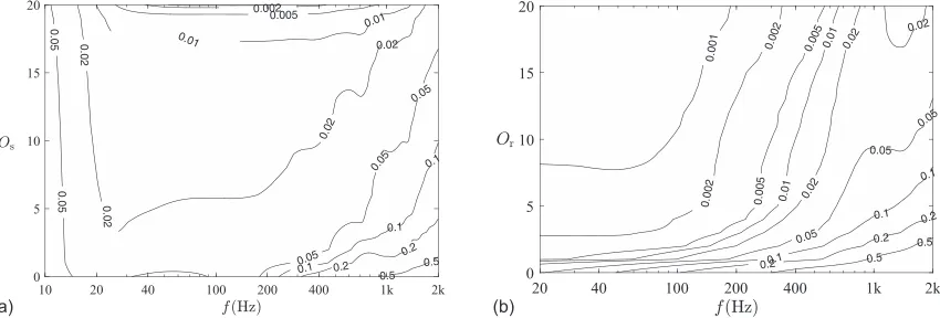
The accuracy achieved by these encoding processes is shown for the Genelec loudspeaker and the HATS in Fig.2; a similar figure for the QSC K8 is included in the supplementary material.63Here, the encoding error is quantified as normalized L2 error, being the L2 norm of the residual between the mea-sured data and the encoded version evaluated on the measure-ment surface, divided by theL2_{norm of the measured data. The} surface integrals involved in theL2 _{norms were approximated} by weighted sums in the same manner as was done in Eq.(9).

In both cases the approximation improves with maxi-mum spherical harmonic orderO, and a higher value ofOis required to maintain the same accuracy as frequency f is increased. The lower right region of the two plots is quite similar, but with slightly smaller residual for the HRTFs. Accuracy deteriorates on the far left of Fig. 2(a)due to the singular nature of spherical Hankel functions at smallkr. In contrast, a clear change in the trend-lines is seen in Fig.2(b)

at 200 Hz; it seems likely that this is caused by the transition between measured and simulated data that was necessary when creating the HRTF library.52

Figure2suggests that the optimal values ofOs. and Or should change with frequency. This was initially attempted, but sharp transitions between orders were visible in the BEM results, hence this approach was discarded. For simplicity, constant values of Os and Or were instead used for all fre-quencies; these were chosen to be Os¼4 and Or ¼10; hence, Ns¼25 andNr¼121. The greater value of Or was chosen to allow the encoding process in Eq.(8)to be tested.

C. BEM

The BEM simulations were performed using BEMþþ23,53,54 version 3.1. This is an open-source BEM library that is invoked from Python scripts, creating a flexi-ble interface that allows the boundary integral operators pro-vided to be assembled in customizable ways. BEMþþ implements a Galerkin BEM algorithm in 3D and includes an ACA solver that accelerates matrix assembly and solution.

For the solution, the Helmholtz equation, BEMþþ pro-vides four standard boundary integral operators that each map, in a different way, a quantityUdefined on a boundary sectionCto a locationx

SfUgðxÞ ¼

ð ð

C

UðyÞGðx;yÞdCy; (10)

Df gU ð Þ ¼x

ð ð

C

U_{ð Þ}y @G

@nyðx;yÞdCy; (11)

Af gU ð Þ ¼x

ð ð

C

U_{ð Þ}y @G

@nxðx;yÞdCy; (12)

Hf gU ð Þ ¼x

ð ð

C

U_{ð Þ}y @

2 G

@nx@nyðx;yÞdCy: (13)

Here, S,D,Aand Hare, respectively, termed: the single-layer potential, the double-single-layer potential, the adjoint double-layer potential, and the hypersingular operator. Note that the definition of Hhas here been written negated com-pared to the convention used in the library. Additionally, an identity operator I fUgðxÞ ¼UðxÞ is also defined. The Python objects representing these operators may be added,

multiplied by each other or scalars, or concatenated to form blocked operators, as required by the problem being studied.

The discretized versions of these boundary operators, for surface to surface mappings, are found using the Galerkin method. Rather than solving a boundary integral equation (BIE) for a finite set of points on the boundary, as is done in the colocation method, this solves the “weak-form” of the BIE on average over the entire boundary, and hence involves a sec-ond surface integral.34A set of weighting functions are chosen to spatially weight this “testing” process and produce each row in the matrix equation; in a Galerkin scheme these are equal to the basis functions used to discretize the boundary quantities. An operator K 2 fS;D;A;H;Ig is therefore mapped to its discrete matrix formK2 fS;D;A;H;Igwith entries given by

Kði;jÞ ¼

ð ð

C

biðxÞKfbjgðxÞdCx: (14)

Here,bj is basis function drawn from the set used to

repre-senting the “radiating” quantity, and bi is a basis function

drawn from the set used to representing the “receiving” quantity that is being “tested”; these sets are not necessarily the same and may be chosen differently on different bound-ary sections or for representing a different quantity. A simi-lar statement maps a user-defined Python function fðxÞ, typically used to compute the incident wave Uinc, onto the “receiving” set of basis functions. This produces a vectorf

with entries defined

fðiÞ ¼

ð ð

C

biðxÞfðxÞdCx: (15)

This interface is extremely flexible, but can be slow for com-plicated functions, since Python is an interpreter language and the functions are evaluated on a per-abscissa basis. In this scheme for instance, fðxÞis typically a Spherical Harmonic basis function (or its spatial derivative), in accordance with the source definition. It will be seen in Sec. IV E that this operation, which is normally assumed to trivially quick com-pared to assembly and solution of the linear system, actually takes the longest due to the complexity of these functions and the slow nature of native Python code compared to the com-piled core libraries that BEMþþin built on.

The KHBIE in Eq.(7)can be written usingDandSas UscatðxÞ ¼ DfUtotalgðxÞ Sf@Utotal=@nygðxÞ. In order to implement the spherical harmonic encoding in Eq.(8), two new boundary operators are defined

Sin

m;nfUgðxÞ ¼

ð ð

C

UðyÞHin

m;nðyxÞdCy; (16)

Din

m;nf gU ð Þ ¼x

ð ð

C

U_{ð Þ}y@H

in

m;n

@ny ðyxÞdCy: (17)

This allows Eq. (8) to be written as Ascat

m;n

¼ikDin

m;nfUtotalgðxrÞ ikS

in

m;nf@Utotal=@nygðxrÞ. It follows that Sin0;0¼ S

ffiffiffiffiffiffi

4p p

=ik and Din

0;0¼ D

ffiffiffiffiffiffi

4p p

=ik, hence Din

m;nandS

in

m;nmay be viewed as a generalization of the

stan-dard operatorsDandS. The discrete form ofDin

m;n andS

in

m;n have matrix entries

given by equations similar to Eqs. (16)and(17)but withbj

appearing in place ofU. These are, unsurprisingly, not built into BEMþþ, but Eq. (15) provides a method to evaluate them. Python functions that compute Hin

m;nðyxrÞ and

@Hin

m;n=@nyðyxrÞmay be passed to the routine that

imple-ments Eq. (15), and the result is a coefficient from the dis-crete matrix form of Sinm;n andD

in

m;n, respectively. Note that

evaluating this in this way is an extremely slow process; the reasons stated above all still apply, but are compounded by the fact that every spherical harmonic order must be evalu-ated separately, and the associevalu-ated Legendre polynomials therein are much more efficiently evaluated simultaneously for allmof an ordernrather than separately. For the verifica-tion purposes herein, however, this inefficiency is tolerated.

The GMRES iterative matrix solver included with SciPy55was used to solve the matrix equations produced using the BEMþþ operators. The ACA accuracy and maximum block size parameters, and the GMRES solver tolerance, were left at their default values of 110–3, 2048 and 110–5, respectively, for scene 3. For scene 9, the former two were reduced to 110–5and 128, respectively, due to some conver-gence issues with matrix solver; this improved accuracy of the matrix approximation at the expense of increased storage and computational cost. Meshing was performed using the open-source meshing tool Gmsh.56,57Maximum element size at any given frequency followed k=8, with a minimum limit chosen to matchk=8 at the crossover frequency.

D. Scene-specific implementation

1. Scene 1H

This scene comprised a loudspeaker above a hard floor in a hemi-anechoic chamber; this was assumed to be per-fectly reflecting. When applying BEM in half-space prob-lems such as this, it is common to apply an image-source principle and reflect the source and all the obstacle bound-aries in the rigid ground plane. Here, there is no additional obstacle, so there is actually no BEM solution at all; there is just the source and the image source, which has reflected directivity. Finding the pressure at a point is as simple as findingUincfrom both sources and summing. Similarly,Am;n

coefficients may be found by applying the translation techni-ques in Ref.22to each source and then summing.

2. Scene 3

This scene included panels that were much thinner in one dimension than the other two. Following standard BEM practice,43,58the obstacle was replaced by one of zero thick-ness lying on its center line. The material had a specific admittanceY that was uniform over both sides of the panel; under this condition the formulation given in Ref.58can be simplified to solving the following pair of coupled BIE for allx2C:DfUtotalgð~ xÞ þ ½ikYS 1

2IfUtotalgð xÞ ¼ UincðxÞ and ½H þ1

combined as a blocked operator in BEMþþ. Here,Utotal and

~

Utotalare respectively the sum of, and the difference between, the pressures acting on the front and back surfaces of the panel. A discontinuous piecewise-constant space was used to discre-tize Utotal and to “test” the first equation. A continuous piecewise-linear space was used to discretize Utotal~ and to “test” the second equation. This arrangement is consistent with the expectation that Utotal~ !0 at the edge of the panel59 and meets the continuity requirements of H.60 _{Pressure at} receiver locations can be evaluated byUscatðxÞ ¼ DfUtotalgð~ xÞ þikYSfUtotalgð xÞ. Following the same logic used to derive this statement,61it can be asserted that the equivalent statement for spherical harmonic coefficients will also hold: Ascat

m;n

¼ikDin

m;nfUtotalgð~ xÞ k2YS

in

m;nfUtotalgð xÞ.

3. Scene 9

Scene 9 is a standard interior admittance problem, so is simpler in its formulation than scene 3. The boundary inte-gral equation to be solved for all x2C is ½D 1

2I þikSYðyÞfUtotalgðxÞ ¼ UincðxÞ. The scattered pressure may be found by UscatðxÞ ¼ ½D þikSYðyÞfUtotalgðxÞ, and equivalently the spherical harmonic coefficients may be found byAscat

m;n ¼ik½D

in

m;nþikS

in

m;nYðyÞfUtotalgðxrÞ:Here, the

only significant complication is thatY is position dependent so cannot be brought outsideS. There are, however, a finite number of materials present in the room, each of which has a uniform value of Y. It is therefore possible to partition the boundary into segments for which Y is uniform and may be brought outside S; this leads to a blocked operator in BEMþþ.Uscat andAscatm;n can be found by evaluating the

con-tribution from each material segment separately and then summing the results.

E. Including measured material data

The boundary data provided in the GRAS database was given as third-octave random-incidence absorption coeffi-cient a. This was converted to an admittance by assuming the material was purely resistive and locally reacting; the lat-ter being a common assumption and the former being accept-able for materials that are fairly hard and reflective,26 such as the MDF in scene 3. Using this, and applying the “55 degree rule,”62 the specific admittance can be found by Y¼cosð558Þ½1pffiffiffiffiffiffiffiffiffiffiffi1a=½1þpffiffiffiffiffiffiffiffiffiffiffi1a. This was then interpolated to the required simulation frequencies using a spline fit assuming ato be constant below the lowest band provided (20 Hz).

This approach was, however, not considered adequate for some of the materials present in scene 9. In particular, it was expected that some materials, e.g., the glazing and door, would exhibit reactive behavior that gave significant losses at low frequencies, and that this was likely to be largely missing from measured material data because it would be non-locally reacting. Attempts were therefore made to fabricate plausible low-frequency resonant damping effects in their place. For example, the fundamental glazing resonant modal frequency was estimated from a plausible pane size, and the frequency of the coincidence dip visible in the measured data. This was implemented by fitting a mass-spring-damper model and the

admittance data produced was combined with that from the measured data using the non-linear crossover technique from Aretzet al.24Missing data for the door was drawn from stan-dard tables62and proprietary field data, then embellished in a similar way. The result was a more plausible room response at low frequencies. For full details of the approaches applied see the code included in the supplementary material.63

IV. RESULTS

In this section, results are presented to validate the pro-posed approach. First, the new process in Eq.(8) that enco-des the pressure around a receiver will be verified. Then the results for the three case studies are validated against mea-surement, including BRIRs for scene 3.

A. Verification of sound field encoding process

Here, the objective is to verify the accuracy ofAinc

n;mand

Ascat

n;m coefficients. Evaluating a metric on these coefficients

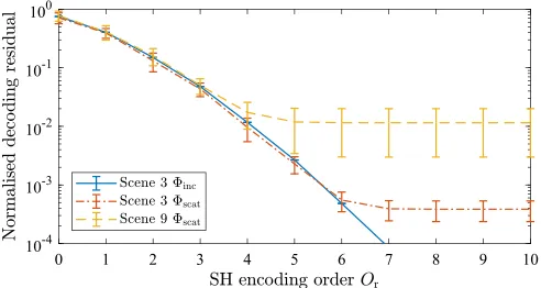
would be the ideal way of quantifying this, but this is com-plicated by the fact that all other known methods of obtain-ing them have limitations too.14–16So here instead, the field has been decoded at a set of points in the domain and the val-ues obtained compared to valval-ues ofUinc andUscatcomputed directly by Eqs. (2) and (7), respectively. 2427 evaluation points were used, arranged quasi-randomly within a sphere of diameter minð1;kÞ centered on xr. The l2 norm of the residual was computed and then normalized by the l2 _norm of the “correct” field; both were windowed with a Hanning window centered on xr. The mean and standard deviation were then computed, averaging with respect to frequency and over loudspeaker position for scene 9, to obtain the trends in Fig.3; error bars indicate6one standard deviation. Note that only frequencies above 343 Hz were included in these statistics; below that, the simulated array became smaller w.r.t.kso the accuracy computed by the metric was unrepresentatively good. More detailed results plotted versus frequency are included in the supplementary material.63

The residual forUincis shown for scene 3 only since the trends for scenes 1 and 9 were identical. This continues to reduce over the full range of Or investigated; what is seen here is just the effect of adding extra terms to the series in Eq. (2), and it appears the Aincn;m coefficients are calculated

accurately for all of these. The standard deviation over fre-quency is extremely small too.

In contrast, the residuals forUscat converge up to some value and then stop; here, decoding accuracy has been lim-ited by error in theAscat

n;m coefficients, indicating the accuracy

of the encoding process; this is around 0.03% for scene 3 and around 1% for scene 9. These are average values, how-ever, and the error bars indicate that quite a significant varia-tion occurs; the maximum residual post-convergence was 0.1% for scene 3 and 7% for scene 9. It is clear from this that the Uscat encoding process in Eq. (8) works quite well for scene 3 but rather less so for scene 9. The reason for this requires further investigation; one possibility is that it occurs because of the sudden change in boundary condition between adjacent materials. The accuracy achieved may still be sufficient for auralization purposes, however; note that the error metric used here is rather stricter than the ‘withinx dB’ criteria that is often used, and it includes phase error.

B. Scene 1H

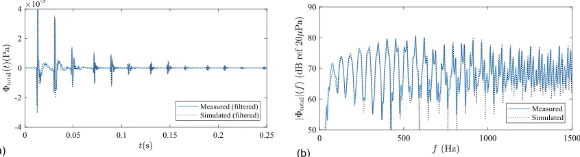
The solution of scene 1H did not involve BEM, so it is included as a means of validating the source directivity model in Eq. (1) and encoding process described in Sec.

III B. Measured and simulated results are compared in Fig.4, which is plotted for loudspeaker position 3 from the database (height 2.6 m angled 60 down) and microphone position 1 (height 1.52 m, 4.1 m from loudspeaker horizontally). In both cases, it is seen that agreement is extremely good. Figure

4(a), in which the measured results have been low-pass fil-tered to match the processing applied to the simulations, shows correct arrival times and polarity, with onset amplitude well matched. Later, the measured result includes a low-frequency oscillation that is absent from the simulated data.

Frequency spectrum agreement in Fig.4(b)is also good, with measured and simulation within 3 dB except at some notches and around 50–100 Hz, where there is a boost in the mea-sured data; this is likely related to the low-frequency oscilla-tion seen in the measured data in Fig.4(a).

C. Scene 3

Scene 3 is an attractive verification case because its sim-ulation involves BEM but it generated a sparse, physically insightful reflection pattern for both RIR and BRIRs. Figure

5shows the RIRs. Again, very good agreement can be seen between simulation and measurement, possibly better than for scene 1H in fact. The onset times, phases and amplitudes of the pulses in Fig.5(a) are all well captured. In Fig.5(b), the interference pattern resulting from the flutter echo is very well matched up to the crossover frequency 1 kHz, after which the simulation begins to deviate from the measured result, perhaps because the BEM mesh is no longer being refined. The results from 1.5 to 2 kHz are hidden from the plot so the lower frequencies can be seen more clearly.

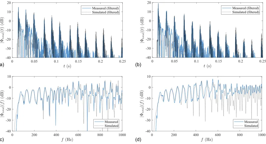
The BRIRs are plotted in Fig. 6. In the time-domain results in Figs. 6(a)and6(b), an instantaneous SPL scale in dB has been used, so that the decay and relative amplitude of the pulse can be see for longer. Again, the pulse times and amplitudes are well-matched and the pattern of which chan-nel is louder matches and makes physical sense. Reflections 1, 4, 7, 10, and 13 are louder in the right ear that faces the loudspeaker, being the original incident wave and its subse-quent reflection back around the system, while others are similarly loud or louder in the left ear. The frequency domain match is less good than was seen in Fig. 5(b); the results can be seen to track each other up to 500 Hz at least. Deviations above that could occur because the simulation FIG. 4. (Color online) RIRs for Scene 1H: (a) versus time (low-pass filtered), (b) versus frequency.

process has combined datasets that have been measured at different times under different conditions. It should be men-tioned that Fig.6hides a detail that the simulated and mea-sured BRIR were negated with respect to one another. Noting, however, that the RIRs in Fig.5matched in sign and that the encoding and decoding was verified in Fig. 3 and Fig. 2(b), it seems most likely that this originates from the HRTF dataset. Auralizations for this scene are included in the supplementary material that accompanies this article.63

D. Scene 9

Scene 9 was included as a more realistic application of the simulation framework. Accuracy is, however, expected to be much poorer than for the other two scenes because: (i) as a closed geometry, the modal and reverberant damping is controlled entirely by boundary absorption mechanisms; (ii) these mechanisms were quite crudely quantified, as discussed in Secs.I B andIII E. Results are shown for source position 2, coordinates [0.12, 2.88, 0.72 m], and microphone position 2, coordinates [0.44,0.15, 0.12 m]; the origin of the coordi-nate system is roughly the center of the room at floor height.

The RIR is shown in the time-domain in Fig.7(a)using an instantaneous SPL scale in dB. It was not expected that the fine detail would match and it does not, but it can be seen

that the general SPL and the decay rate match well. Figure

7(b)shows the same data in the frequency domain, display-ing 0–250 Hz since the modal density above this means no discernable features are observable. The general SPL trend is captured quite well up to 170 Hz, with matches between individual modal frequencies identifiable. That some of these peaks match quite well in SPL and bandwidth is impressive, since this is largely dictated by the boundary absorption data, which was heavily extrapolated. BRIR results are not shown since little detail can be discerned graphically, but auralizations for this scene are included in the supplementary material that accompanies this article.63

E. Computation times

Computing times for scenes 3 and 9 are shown in Figs.

8(a) and 8(b), respectively. Here, the main observation is that all trends scale with #DOF (plotted against the right-hand axis). This is expected for the “Setup RHS” and the “Receiver encoding” tasks, being processes 3 and 5 in Fig.1, respectively, but not for “Setup LHS” and “Solve,” together being process 4 in Fig. 1. In a conventional BEM, these would scale with #DOF2, so it is clear that the ACA solver has achieved significant computational savings. In contrast, “Setup RHS” and “Receiver encoding” would normally be FIG. 6. (Color online) BRIRs for Scene 3: (a) left ear versus time (low-pass filtered), (b) right ear versus time (low-pass filtered), (c) left ear versus frequency, (d) right ear versus frequency.

expected to be by far the quickest steps but, due to the afore-mentioned implementation in as interpreted Python func-tions, they are much slower than the optimized, compiled core of the library. This should not however be taken as rep-resentative of the new source and receiver mapping techni-ques described herein; it is merely due to implementation compromises and an efficient, compiled implementation of them could be readily achieved.

V. CONCLUSIONS AND FURTHER WORK

This paper has proposed a framework for low-frequency room acoustic simulation, echoing similar frameworks that have been proposed for geometrical acoustics models at high-frequencies. A key component of this was the mapping pro-posed by Hargreaves and Lam18to encode boundary data to spherical harmonic descriptions of the pressure field around a receiver, and verification data, results, and auralizations using that are provided herein. The full simulation chain was vali-dated using three case studies drawn from the GRAS database, one of which was hemi-anechoic, one fully-anechoic, and one a real room. The simulations were seen to match measurement well for the hemi-anechoic and fully-anechoic cases, but less so for the room; this was expected since standardized means of quantifying boundary material data are not sufficient for the simulation algorithms brought to bear. Clearly, this latter aspect is a limiting factor in the simulation chain, and one that must be addressed if room acoustic simulations are to move from being plausible to reliably physically accurate.

In terms of future work, it is clear that the current imple-mentation of the new source and receiver mappings is extremely inefficient, and an optimized compiled version would be required for serious usage. It is also clear that repeated use of a frequency-domain BEM code followed by IFFT is not an efficient way of generating an impulse response; convolution quadrature46 or multifrequency49,50 approaches would be far more efficient. More research is required to set bounds on the accuracy of the new pressure field encoding process, since this was seen to vary with the problem modelled. Finally, these simulations have shown that numerical models can closely match reality when the input data is of a good quality but that they deviate when it is not. Hence improved techniques to characterize materials, ideallyin situ, are required.

ACKNOWLEDGMENTS

This work was supported by the UK Engineering and Physical Sciences Research Council (Grant Nos. EP/ J022071/1 and EP/K000012/1 “Enhanced Acoustic Modelling for Auralisation using Hybrid Boundary Integral Methods”). All data supporting this study are provided as supplementary material accompanying this paper. We would like to thank the team at RWTH Aachen and TU Berlin for kindly providing advanced access to their detailed Ground Truth for Room Acoustic Simulation (GRAS) database, in particular Lukas Asp€ock and Fabian Brinkmann for their generous support during this process.

1_{M. Kleiner, B.-I. Dalenb€ack, and P. Svensson, “Auralization—An}

over-view,” J. Audio Eng. Soc.41, 861–875 (1993).

2

N. Xiang and J. Blauert, “Binaural scale modelling for auralisation and prediction of acoustics in auditoria,”Appl. Acoust.38, 267–290 (1993).

3

L. Savioja and U. P. Svensson, “Overview of geometrical room acoustic modeling techniques,”J. Acoust. Soc. Am.138, 708–730 (2015).

4

E. Granier, M. Kleiner, B.-I. Dalenb€ack, and P. Svensson, “Experimental auralization of car audio installations,” J. Audio Eng. Soc.44, 835–849 (1996).

5

M. Vorl€ander, “Computer simulations in room acoustics: Concepts and uncertainties,”J. Acoust. Soc. Am.133, 1203–1213 (2013).

6

T. Sakuma, S. Sakamoto, and T. Otsuru, Computational Simulation in Architectural and Environmental Acoustics (Springer Japan, Tokyo, 2014).

7_{M. Aretz and M. Vorl€ander, “Combined wave and ray based room}

acous-tic simulations of audio systems in car passenger compartments, Part II: Comparison of simulations and measurements,”Appl. Acoust.76, 52–65 (2014).

8

L. A. T. Jimenez, S. R. Sanchez, J. O. Villegas, and A. L. Ciro, “Subjective assessment of auralizations created by means of geometrical acoustics and finite element numerical methods” in Proceedings of the International Congress on Sound and Vibration, London, UK (23–27, 2017).

9

J. E. Summers, K. Takahashi, Y. Shimizu, and T. Yamakawa, “Assessing the accuracy of auralizations computed using a hybrid geometrical-acoustics and wave-geometrical-acoustics method,” J. Acoust. Soc. Am.115, 2514 (2004).

10

M. A. Poletti, “Three-dimensional surround sound systems based on spherical harmonics,” J. Audio Eng. Soc.53, 1004–1025 (2005).

11

J. Ahrens, “The single-layer potential approach applied to sound field syn-thesis including cases of non-enclosing distributions of secondary sources,” Ph.D. thesis, TU Berlin, Berlin, 2010.

12

S. Pelzer, M. Pollow, and M. Vorl€ander, “Continuous and exchangable directivity patterns in room acoustic simulation,” inProceedings of DAGA 38, Darmstadt, Germany (March 19–22, 2012).

13_{P. Samarasinghe, T. Abhayapala, M. Poletti, and T. Betlehem, “An}

effi-cient parameterization of the room transfer function,”IEEE/ACM Trans. Audio Speech Lang. Process.23, 2217–2227 (2015).

14

A. Southern, D. T. Murphy, and L. Savioja, “Spatial encoding of finite dif-ference time domain acoustic models for auralization,” IEEE Trans. Audio. Speech. Lang. Process.20, 2420–2432 (2012).

15

D. Gomez, J. Astley, and F. Fazi, “Low frequency interactive auralization based on a plane wave expansion,”Appl. Sci.7, 558 (2017).

16

J. Sheaffer, M. van Walstijn, B. Rafaely, and K. Kowalczyk, “Binaural reproduction of finite difference simulations using spherical array proc-essing,”IEEE/ACM Trans. Audio Speech Lang. Process.23, 2125–2135 (2015).

17

R. Mehra, L. Antani, S. Kim, and D. Manocha, “Source and listener direc-tivity for interactive wave-based sound propagation,” IEEE Trans. Vis. Comput. Graph.20, 495–503 (2014).

18

J. A. Hargreaves and Y. W. Lam, “An energy interpretation of the kirchhoff-helmholtz boundary integral equation and its application to sound field synthesis,”Acta Acust. united Ac.100, 912–920 (2014).

19_{E. Hulsebos, D. de Vries, and E. Bourdillat, “Improved microphone array}

configurations for auralization of sound fields by Wave Field Synthesis,” inProceedings of the AES Convention, Amsterdam, the Netherlands (May 12–15, 2001).

20

I. Harari and T. J. R. Hughes, “A cost comparison of boundary element and finite element methods for problems of time-harmonic acoustics,” Comput. Methods Appl. Mech. Eng.97, 77–102 (1992).

21_{T. J. Cox, “Prediction and evaluation of the scattering from quadratic}

resi-due diffusers,”J. Acoust. Soc. Am.95, 297–305 (1994).

22_{N. Gumerov and R. Duraiswami, Fast Multipole Methods for the}

Helmholtz Equation in Three Dimensions, 1st ed. (Elsevier Science, Amsterdam, the Netherlands, 2005).

23

T. Betcke, E. van’t Wout, and P. Gelat, “Computationally efficient bound-ary element methods for high-frequency helmholtz problems in unbounded domains,” in Modern Solvers for Helmholtz Problems

(Birkh€auser, Germany, 2017), pp. 215–243.

24_{M. Aretz, R. N€othen, M. Vorl€ander, and D. Schr€oder, “Combined}

broad-band impulse responses using fem and hybrid ray-based methods,” inEAA Symposium on Auralization, Espoo, Finalnd (June 15–17, 2009).

25

M. Aretz, “Specification of realistic boundary conditions for the FE simu-lation of low frequency sound fields in recording studios,”Acta Acust. united Ac.95, 874–882 (2009).

26_{M. Aretz, “Combined wave and ray based room acoustic simulations of}

small rooms,” Ph.D. thesis, RWTH Aachen, Aachen, Germany, 2012.

27

M. Aretz and M. Vorl€ander, “Combined wave and ray based room acous-tic simulations of audio systems in car passenger compartments, Part I: Boundary and source data,”Appl. Acoust.76, 82–99 (2014).

28_{A. Southern, S. Siltanen, D. T. Murphy, and L. Savioja, “Room impulse}

response synthesis and validation using a hybrid acoustic model,”IEEE Trans. Audio. Speech. Lang. Process.21, 1940–1952 (2013).

29

F. Brinkmann, L. Asp€ock, D. Ackermann, R. Opdam, M. Vorlaender, and S. Weinzierl, “First international round robin on auralization: Concept and database,”J. Acoust. Soc. Am.141, 3856–3856 (2017).

30

L. Asp€ock, F. Brinkmann, D. Ackerman, S. Weinzierl, and M. Vorl€ander, “GRAS—Ground Truth for Room Acoustical Simulation,” https:// dx.doi.org/10.14279/depositonce-6726(Last viewed March 19, 2018).

31_{S. Bilbao and B. Hamilton, “Directional source modeling in wave-based}

room acoustics simulation,” inProceedings of the 2017 IEEE Workshop on Applications of Signal Processing to Audio and Acoustics, New Paltz, NY (October 15–18, 2017).

32_{S. Sakamoto and R. Takahashi, “Directional sound source modeling by}

using spherical harmonic functions for finite-difference time-domain ana-lysis,”Proc. Meet. Acoust.19, 015129 (2013).

33

F. Georgiou and M. Hornikx, “Incorporating directivity in the Fourier pseudospectral time-domain method using spherical harmonics,” J. Acoust. Soc. Am.140, 855–865 (2016).

34

S. Marburg, “Boundary element method for time-harmonic acoustic prob-lems,” in Computational Acoustics (Springer International Publishing, New York, 2018), pp. 69–158.

35_{E. G. Williams, Fourier Acoustics: Sound Radiation and Nearfield}

Acoustical Holography(Academic Press, San Diego, CA, 1999).

36

G. Weinreich, “Method for measuring acoustic radiation fields,”J. Acoust. Soc. Am.68, 404–411 (1980).

37

M. J. Evans, J. A. S. Angus, and A. I. Tew, “Analyzing head-related trans-fer function measurements using surface spherical harmonics,”J. Acoust. Soc. Am.104, 2400–2411 (1998).

38_{F. W. J. Olver, A. B. Olde Daalhuis, D. W. Lozier, B. I. Schneider, R. F.}

Boisvert, C. W. Clark, B. R. Miller, and B. V. Saunders, “NIST digital

library of mathematical functions,” http://dlmf.nist.gov/ (Last viewed January 24, 2018).

39

M. Pollow, K.-V. Nguyen, O. Warusfel, T. Carpentier, M. M€uller-Trapet, M. Vorl€ander, and M. Noisternig, “Calculation of head-related transfer functions for arbitrary field points using spherical harmonics decom-position,”Acta Acust. united Ac.98, 72–82 (2012).

40

M. Melon, C. Langrenne, P. Herzog, and A. Garcia, “Evaluation of a method for the measurement of subwoofers in usual rooms,”J. Acoust. Soc. Am.127, 256–263 (2010).

41

Klippel GmbH, “Near field scanner system,” https://www.klippel.de/prod-ucts/rd-system/modules/nfs-near-field-scanner.html (Last viewed August 1, 2018).

42

J. A. Hargreaves and Y. W. Lam, “Corrigendum to ‘An energy interpreta-tion of the Kirchhoff-Helmholtz boundary integral equainterpreta-tion and its applica-tion to sound field synthesis,’”Acta Acust. united Ac.104(6), 1134 (2018).

43_{R. Martinez, “The thin-shape breakdown (TSB) of the Helmholtz integral}

equation,”J. Acoust. Soc. Am.90, 2728–2738 (1991).

44

Y. Sakurai and K. Ishida, “Multiple reflections between rigid plane pan-els,”J. Acoust. Soc. Jpn.3, 183–190 (1982).

45_{E. Brand~ao, A. Lenzi, and S. Paul, “A review of thein situimpedance and}

sound absorption measurement techniques,”Acta Acust. united Ac.101, 443–463 (2015).

46

S. A. Sauter and M. Schanz, “Convolution quadrature for the wave equa-tion with impedance boundary condiequa-tions,” J. Comput. Phys. 334, 442–459 (2017).

47

J. A. Hargreaves and T. J. Cox, “A transient boundary element method model of Schroeder diffuser scattering using well mouth impedance.,” J. Acoust. Soc. Am.124, 2942–2951 (2008).

48

T. Okuzono, T. Yoshida, K. Sakagami, and T. Otsuru, “An explicit time-domain finite element method for room acoustics simulations: Comparison of the performance with implicit methods,” Appl. Acoust. 104, 76–84 (2016).

49_{O. von Estorff, S. Rjasanow, M. Stolper, and O. Zaleski, “Two efficient}

methods for a multifrequency solution of the Helmholtz equation,” Comput. Vis. Sci.8, 159–167 (2005).

50_{J.-P. Coyette, C. Lecomte, J.-L. Migeot, J. Blanche, M. Rochette, and G.}

Mirkovic, “Calculation of vibro-acoustic frequency response functions using a single frequency boundary element solution and a Pade expansion,” Acta Acust. united with Ac.85, 371–377 (1999).

51_{F. Brinkmann, A. Lindau, and S. Weinzierl, “A high resolution}

head-related transfer function database including different orientations of head above the torso,” inProceedings of the AIA-DAGA, Merano, Italy (March 18–21, 2013).

52_{F. Brinkmann, A. Lindau, M. M€uller-Trapet, M. Vorl€ander, and S. Weinzierl,}

“Cross-validation of measured and modeled head-related transfer functions,” inProceedings of DAGA 2015, N€urnberg, Germany (March 16–19, 2015).

53

W.Smigaj, T. Betcke, S. Arridge, J. Phillips, and M. Schweiger, “Solving boundary integral problems with BEMþþ,” ACM Trans. Math. Softw. 41, 1–40 (2015).

54

S. Arridge, T. Betcke, M. Scroggs, and E. van’t Wout, “bempp services,” www.bempp.org, (Last viewed December 14, 2017).

55_{E. Jones, E. Oliphant, and P. Peterson, “SciPy: Open source scientific tools}

for Python,”http://www.scipy.org/(Last viewed December 14, 2017).

56

C. Geuzaine and J.-F. Remacle, “Gmsh: A 3-D finite element mesh gener-ator with built-in pre- and post-processing facilities,” Int. J. Numer. Methods Eng.79, 1309–1331 (2009).

57

C. Geuzaine and J.-F. Remacle, “Gmsh: A three-dimensional finite ele-ment mesh generator with built-in pre- and post-processing facilities,” http://gmsh.info/(Last viewed December 14, 2017).

58_{Y. Yasuda and T. Sakuma, “Boundary element method,” in}

Computational Simulation in Architectural and Environmental Acoustics

(Springer Japan, Tokyo, 2014), pp. 79–115.

59

D. P. Hewett and U. P. Svensson, “The diffracted field and its gradient near the edge of a thin screen,”J. Acoust. Soc. Am.134, 4303–4306 (2013).

60_{G. Krishnasamy, L. W. Schmerr, T. J. Rudolphi, and F. J. Rizzo,}

“Hypersingular boundary integral equations: Some applications in acous-tic and elasacous-tic wave scattering,”J. Appl. Mech.57, 404–414 (1990).

61_{T. Terai, “On calculation of sound fields around three dimensional objects}

by integral equation methods,”J. Sound Vib.69, 71–100 (1980).

62

T. J. Cox and P. D’Antonio,Acoustic Absorbers and Diffusers: Theory, Design and Application, 2nd ed. (Taylor & Francis, London, 2009).

63_{See supplementary material athttps://doi.org/10.1121/1.5096171 for}