Munich Personal RePEc Archive
State capacity and long-run performance
Dincecco, Mark and Katz, Gabriel
IMT Lucca Institute for Advanced Studies
23 April 2012
Online at
https://mpra.ub.uni-muenchen.de/42316/
State Capacity and Long-Run Performance
∗
Mark Dincecco
†Gabriel Katz
‡October 29, 2012
Abstract
We present new evidence about the long-term links between state capacity and eco-nomic performance. Our database is novel and spans 11 countries and 4 centuries in Eu-rope, the birthplace of modern economic growth. Using standard panel data methods, we find that the performance impacts of states with modern extractive and productive capabilities are significant, large, and robust to a wide variety of specifications, controls, and modeling techniques.
Keywords: political regime types, state capacity, public services, economic performance, European history.
JEL codes: C33, H11, H41, N43, O23, P48.
∗We thank seminar participants at Berkeley, Bocconi, Caltech, Copenhagen, the 2012 Economic History
Association Annual Meeting, the Inter-American Development Bank, the Juan March Institute, the London School of Economics, the 2012 Nemmers Prize Conference, Stanford, Toulouse, Utrecht, and Yale for valuable comments, and Rui Esteves, Giovanni Federico, Klas Fregert, Michael Pammer, and Mark Spoerer for data. Mark Dincecco also thanks Barry Eichengreen for his hospitality during an extended visit to the Berkeley Economic History Laboratory, where part of this paper was written. He gratefully acknowledges financial support from National Science Foundation Grant SES-1227237.
†IMT Lucca Institute for Advanced Studies; email: [email protected]
1
Introduction
Standard economic theory assumes that states can tax at will and commit funds to a broad set of military and civilian goods. However, effective states are only a recent his-torical development.1 Effective states, furthermore, represent just a fraction of modern nations. Like their historical predecessors, today’s developing states often confront
prob-lems of low revenues and unproductive expenditures.2 To explain why some countries
achieve long-run economic growth but others do not, a clear understanding of state ca-pacity is therefore critical.
An early, case-based literature in political science highlights the role of state capacity
in development, and state capacity has now become a key concern of economists.3 A
recent major work by Besley and Persson (2011) defines state capacity in terms of two complementary capabilities that enable the state to act. The first concerns the state’s ex-tractive role as a tax collector and the second its productive role as a provider of public services (e.g., transportation networks, courts). Besley and Persson argue that state ca-pacity – the combined extractive and productive capabilities of the state – forms a critical part of development clusters that vary closely with income levels.
The main task of the new economics literature has been to expand standard theory to incorporate state capacity issues. However, there are still relatively few quantitatively rigorous empirical works, whether in economics or political science, about the long-term links between state capacity and economic performance. To address this important gap, this paper examines the economic impacts of fundamental political transformations that resolved long-standing state capacity problems in Europe, the birthplace of modern eco-nomic growth.
We argue that sovereign governments in European history faced two basic political problems: fiscal fragmentation and absolutism. Although rulers had weak authority over taxation, they had strong control over expenditures. Under this equilibrium, rev-enues were low and executives typically spent available funds on military adventures rather than on public services with broad economic benefits.
1See Hintze (1906), Tilly (1975, 1990), Mathias and O’Brien (1976), Levi (1988), Brewer (1989), Hoffman
and Rosenthal (1997), Epstein (2000), O’Brien (2001, 2011), Dincecco (2011), Karaman and Pamuk (2011), and Rosenthal and Wong (2011).
2For state capacity problems in sub-saharan Africa, see Migdal (1988), Herbst (2000), and Bates (2001). By
contrast, states have played key roles in the successful development experiences of Asian Tiger nations. See Wade (1990) and Kang (2002).
3For political science works, see Footnote 2. For economics, see Acemoglu et al. (2004), Acemoglu (2005),
The political transformations that we study fit squarely within Besley and Persson’s (2011) conceptual framework of economic development. We argue that the implementa-tion of uniform tax systems at the naimplementa-tional level – which we call “fiscal centralizaimplementa-tion” – enabled European states to effectively fulfill their extractive role. This transformation typically occurred swiftly and permanently from 1789 onward. Similarly, we argue that the establishment of parliaments that could monitor public expenditures at regular inter-vals – called “limited government” – enabled them to effectively fulfill their productive role. This transformation typically occurred decades after fiscal centralization over the nineteenth century. By the mid-1800s, most European states had achieved “modern” ex-tractive and productive capabilities, implying that they could gather large tax revenues and effectively channel funds toward non-military public services.
We argue that these critical improvements in state capacity had strongly positive per-formance impacts. To rigorously develop our claim, we perform a panel regression anal-ysis on a novel database that spans eleven countries from the height of the Old Regime in 1650 to the eve of World War I in 1913. Our main specification uses a standard difference-in-differences approach. We first model the extractive and productive capabilities of states as a function of political regime type, country fixed effects that account for un-observed time-invariant, country-level heterogeneity, time fixed effects that account for common shocks, time-varying controls including external and internal conflicts and state antiquity, and country-specific time trends. We then model economic performance as a function of state capacity. For robustness, we also use two alternative specifications to difference-in-differences. The first includes a lagged dependent variable to account for persistence in fiscal and economic outcomes. The second uses a GMM approach, en-abling us to account for simultaneity and omitted variable bias alike. We discuss poten-tial threats to inference at length in Section 5.
per-cent increase in per capita revenues led to a 0.384 to 0.833 perper-centage point increase in the subsequent five-year growth rate of per capita GDP. Similarly, a 1 percent increase in per capita non-military expenditures led to a 1.261 to 3.272 percentage point increase in the subsequent GDP growth rate. Given that average growth rates ranged from 3 to 5 percent over our sample period, the magnitudes of these performance impacts are substantial.
Our paper is related to the literature that examines the links between historical insti-tutional factors and long-run economic performance, including Engerman and Sokoloff (1997), La Porta et al. (1998), Hall and Jones (1999), Acemoglu et al. (2001, 2002, 2005a), Banerjee and Iyer (2005), and Nunn (2008). None of these works, however, focus on state capacity.4 Furthermore, this literature does not typically identify just how history
matters (Nunn, 2009).5 Our paper tests a specific mechanism – namely, the impacts of
effective revenue extraction and spending – through which state capacity improvements have long-term economic impacts. Overall, our macro-oriented approach complements microeconomic research that uses randomized controlled experiments to test whether specific policy interventions are effective (Duflo et al., 2007).
Our paper is also related to the literature that argues that the state was an active participant in the development of modern capitalist systems, including Gerschenkron (1966), Magnusson (2009), and O’Brien (2011). We provide a data-intensive, rigorous counterpart to these works. Our paper thus contributes to the debate regarding the in-stitutional origins of the Industrial Revolution (Acemoglu et al., 2005b, Mokyr, 2008).
The rest of the paper proceeds as follows. Section 2 describes the historical back-ground and Section 3 develops our theoretical implications. Section 4 presents the data and descriptive statistics, a case study of France, a core sample country, and structural breaks tests. Section 5 discusses the econometric methodology. Section 6 reports the results of our estimations for the impacts of political regimes on state capacity, includ-ing the placebo tests. Section 7 reports the results for the impacts of state capacity on economic performance. Section 8 concludes.
4One exception is Bockstette et al. (2002), which investigates the economic impacts of early statehood. They
find a strong positive link between state antiquity and current development. Similarly, Dincecco and Prado (2012) find a strong positive relationship between fiscal capacity and performance. They use historical war casualties to instrument for current fiscal institutions.
5A recent exception is Dell (2010), which argues that public goods provision by large landowners in
2
Historical Background
This section characterizes the two fundamental political transformations that resolved key state capacity problems in European history. We argue that fiscal centralization al-lowed states to effectively fulfill their extractive role and limited government their pro-ductive one.6
2.1
Fiscal Centralization
Most polities in Europe were fiscally fragmented before the nineteenth century. Contrary to conventional wisdom, monarchs confronted a host of incumbent local institutions that reduced their fiscal powers. Epstein (2000, pp. 13-14) writes that
decades of research on pre-modern political practices. . . has shown how “ab-solutism” was a largely propagandistic device devoid of much practical sub-stance. . . The strength of a monarch’s theoretical claims to absolute rule was frequently inversely proportional to his de facto powers.
One general feature of fragmented states was the close relationship between local tax control and political autonomy. Provincial elites thus had strong incentives to oppose fiscal reforms that threatened traditional tax rights. The result was a classic public goods problem. Since each local authority attempted to free-ride on the tax contributions of others, the revenues that national governments could extract per capita were low.
To resolve the problem of local tax free-riding, executives had to gain the fiscal au-thority to impose standard tax menus rather than bargain place by place over individual rates. So long as states equalized rates across provinces at relatively high levels, govern-ment revenues per head rose.
A clear and simple definition of fiscal centralization facilitates comparison across states. We define that the centralization process was completed the year that the national government first secured its revenues through a standard tax system with uniform rates throughout the country.7
All pre-centralized regimes were classified as entirely fragmented, even for states where fiscal divisions were relatively small. This choice implies that some regimes that
6Our account follows Dincecco (2011, chs. 2-3), who also provides sources.
7This definition does not imply that central governments became tax monopolists. The history of the United
were counted as fully fragmented will encompass data associated with higher per capita revenues. Average improvements after fiscal centralization will therefore be smaller than otherwise. Systematic underestimation of the fiscal impacts of centralization biases the data against the hypothesis that fiscal centralization increased revenues. The results of our analysis will thus be stronger than otherwise if they still indicate that fiscally central-ized regimes had significant positive fiscal impacts.
Table 1 displays the dates of fiscal centralization across sample countries. The Nor-man Conquest of 1066 undercut provincial authority in England and established a uni-formity of laws and customs that other states did not achieve until much later.8 Struc-tural changes took place swiftly and permanently in many parts of continental Europe after the tumultuous fall of the Old Regime. The National Assembly transformed the tax system in France by eliminating traditional privileges at the start of the Revolution (1789-99). Napoleon completed this process after taking power in 1799. The First French Republic conquered the Low Countries in 1795, and the Southern Netherlands including Belgium became French departments. The Batavian Republic, the successor to the Dutch Republic, established a national system of taxation under French rule in 1806. French conquest at the start of the 1800s was also the major catalyst for fiscal change on the Italian peninsula. France annexed Piedmont in 1802. Finally, Prussia undertook major administrative reforms including fiscal centralization after its loss to France in the Battle of Jena-Auerstedt in 1806.
Although Napoleon defeated Austria in 1805 and invaded Portugal in 1807 and Spain in 1808, he implemented incomplete administrative changes in those territories. Fiscal centralization did not take place in the Austrian Empire until after the 1848 revolutions, which had important implications for bureaucratic structures. Most notably, the central government in Vienna began to implement an effective Cisleithanian tax system in Hun-gary.9 Fiscal centralization also occurred in the 1840s in Spain during a period of major reforms. Significant fiscal change in Portugal took place in the 1850s. The 1859 reform led to the centralization and regulation of government accounts.
8England conjoined with Wales in 1536. The Act of Union of 1707 conjoined Scotland. A similar Act
con-joined Ireland in 1800 (the Irish Free State was established in 1922). For consistency, the term ”England” rather than “Great Britain” or the “United Kingdom” is used throughout the text. However, we must distinguish be-tween medieval English fiscal and political institutions and British ones. Brewer (1989, pp. 5-6) writes: “There was certainly an English medieval state, made from a Norman template, but not a British one. . . Nevertheless the English core of what was eventually to become the British state was both geographically larger and better administrated than its French equivalent.”
9Austria and Hungary were the largest territories of the Austrian Empire (1804-67). The Compromise of
Pre-modern fiscal structures remained in Scandinavia through much of the 1800s. Major changes did not occur until the second half of the nineteenth century or later. The 1861 reform in Sweden abolished the traditional system of dividing tax subjects into different classes with many sub-groups and rules for fixed contributions. Similarly, the 1903 reform in Denmark eliminated traditional tax structures and introduced a modern income tax with standard, country-wide rates.
2.2
Limited Government
Although rulers spent government funds as they pleased, elites in national parliaments exercised tax authority. Hoffman and Rosenthal (1997) argue that the one true goal of absolutist monarchs was to wage war for personal glory and for homeland defense. A key reason was the problem of royal moral hazard in warfare (Cox, 2011). In Hoffman’s (2009, p. 24) words, monarchs
overspent on the military and provided more defense than their citizens likely desired. But they had little reason not to. Victory. . . won them glory, enhanced reputations, and resources. . . Losses never cost them their throne.
Since parliamentary elites feared that executives would spend additional revenues in wasteful ways like foreign military adventures, they demanded the power of budgetary oversight before raising new taxes. To evade parliament, rulers resorted to fiscal preda-tion, which reinforced the fear that they could not be trusted. Parliamentary elites thus resisted tax requests and revenues were low.
Regular control over state budgets firmly established the fiscal supremacy of par-liament. In turn, the likelihood of poor spending choices by executives fell. Although structural reforms implied that rulers would receive greater revenues, the surrender of budgetary control was the only credible way for executives to guarantee that a portion of the new funds would be used on non-military public services that parliamentary elites desired.
Even if rulers and elites each had incentives to set new rules over government ex-penditures, however, institutional reform was notoriously difficult. Limited government was typically established at critical junctures that came at the confluence of idiosyncratic shocks. For pre-1789 France, for instance, Hoffman and Rosenthal (1997, pp. 33-4) write:
had stitched the kingdom together by according judicial privileges to power-ful interest groups. Abolishing their privileges, even for the sake of judicial rationality, was out of the question. . . It is no surprise then that legal reform required a bloody revolution.
The next subsection further examines the role of critical junctures and institutional change. A valid depiction of parliamentary authority must capture its real power to act on the budget. It must also be clear and simple enough to apply across states. The substance of our definition derives from the classic work of North and Weingast (1989). We de-fine that limited government was established the year that parliament gained the stable constitutional right to control the national budget on an annual basis. The requirement that parliament’s power of the purse held for at least two consecutive decades ensures stability. To make the coding as objective as possible, years and regimes for which there are widespread academic consensus were chosen. There is a close correspondence be-tween our coding scheme and the schemes of De Long and Shleifer (1993), Acemoglu et al. (2005a), and the Polity IV Database of Jaggers and Marshall (2008), though none of these schemes fit the particular demands of our analysis.10 In total, these three features - a regular right by parliament to manage budgets, regime stability, and scholarly agree-ment - imply that our coding of limited governagree-ment parallels the standard that North and Weingast introduced.
Selecting early dates to define political regimes as limited implies that average out-comes under parliamentary regimes will be worse than otherwise. For instance, one can argue that a stable form of limited government did not truly emerge in Germany until af-ter World War II (the Weimar Republic endured for only 14 years, from 1918 to 1933) or in Spain until after the death of Franco in 1975. If this were the case, then the correct coding would be to categorize the pre-twentieth-century Prussian and Spanish regimes as ab-solutist. Similar arguments can be made for Italy and Portugal. Since public finances in Europe typically improved over time, the choice of early dates means that some regimes classified as limited will encompass data associated with lower per capita non-military spending. Average improvements after parliamentary reforms will therefore be smaller than otherwise. Systematic underestimation of the fiscal impacts of limited government
10De Long and Shleifer (1993) use three measures: a binary indicator of absolutist versus non-absolutist
biases the data against the hypothesis that parliamentary reforms increased non-military spending. Any results of our analysis that still indicate that limited government had significant positive impacts on spending habits will thus be stronger than otherwise.
Furthermore, the establishment of limited government was not necessarily irreversible. There were some instances of switching back and forth with absolutism over the 1800s. As described, our definition sets a stability threshold by requiring that parliamentary budgetary authority held for at least two straight decades.
Nineteenth-century France illustrates our coding methodology. The Bourbon monar-chy was restored after the final defeat of Napoleon in 1815. This regime was constitu-tional in name alone. In 1830, King Charles X dissolved parliament, manipulated the electorate in favor of his supporters, placed the press under government control, and called for new elections. These measures incited the July Revolution the next day. King Louis Philip, the replacement for the deposed monarch, agreed to follow constitutional principles, but his tenure was beset by the economic crisis of the mid-1840s and ended with the Revolution of 1848. Since the reign of Louis Philip endured for less than two decades, our benchmark scheme does not code the July regime as limited. However, the case study in Section 4 accounts for its fiscal impacts. Napoleon III, who was elected president of the Second Republic in 1848, staged a successful coup in 1851 and estab-lished an authoritarian regime (called the Second Empire) that lasted nearly 20 years. The emperor was captured during the Franco-Prussian War (1870-1) and the provisional government of the Third Republic was quickly formed. This regime was consolidated in the aftermath of the conflict, which France lost, and endured for 70 years until the German invasion of 1940. Since the Third Republic best satisfies the triple criteria of par-liamentary regularity, stability, and scholarly consensus, our coding methodology dates the emergence of limited government in France to 1870.
Table 2 displays the dates of limited government across sample countries. Parlia-mentary reforms typically occurred decades after fiscal centralization over the nine-teenth century. Belgium was established as a constitutional monarchy after revolting and declaring independence from the Netherlands in 1830. In the Netherlands itself, a new constitution that required the executive to submit annual budgets for parliamen-tary approval was promulgated during the Year of Revolutions in 1848. Kings Charles Albert of Piedmont and Frederick William IV of Prussia also granted liberal
constitu-tions in 1848.11 The Compromise of 1867, which established Austria and Hungary as
11Tilly (1966) argues that there were binding fiscal constraints in Prussia from 1848 onward, although the
distinct political entities, marked the start of the constitutional era in Austria following the Austro-Prussian War (1866). Spain fought several civil wars over the 1800s. A stable parliamentary regime was established in 1876 following the Third Carlist War (1872-6).
By contrast, limited government and fiscal centralization took place within a decade of each other in Sweden and Portugal. Although Sweden enacted a constitution in 1809, the executive retained absolute veto authority and parliament met only once every five years. The parliamentary reform of 1866, which replaced the traditional Diet of Estates with a modern bicameral legislature, established limited government. This institutional change occurred five years after fiscal centralization in 1861. Like Spain, Portugal fought a series of civil wars over the nineteenth century. A stable constitutional regime was established in 1851, eight years before fiscal centralization in 1859.
There are two cases in which limited government was implemented well in advance of fiscal centralization. In Denmark, King Frederick VII renounced his absolutist powers and established a two-chamber parliament after the political revolutions of 1848. Fis-cal centralization did not take place in Denmark until 1903. The Dutch Republic (1572-1795) is typically classified as constitutional (De Long and Shleifer, 1993, Acemoglu et al., 2005a, Stasavage, 2005). Recall, however, that the Republic was fiscally fragmented at the national level.
2.3
Quasi-Random Variation
The historical evidence suggests that it is plausible to treat political transformations as the result of quasi-random variation or shocks. As described, the establishment of uniform tax systems was often the result of radical, externally imposed reform. In the German territories, in the Low Countries, and on the Italian (and to a lesser extent, the Iberian) peninsula, fiscal centralization was the result of French conquest from 1792 on-ward. As O’Brien (2011a, p. 436) writes:
It seems that only the exogenous shocks of the kind delivered by. . . the out-comes that flowed from the French Revolution (1789-1815) led to serious re-forms to the fiscal constitutions of other ancien r´egimes on the mainland.
A similar logic holds for the establishment of centralized institutions in England follow-ing the Norman Conquest in the eleventh century.
uniform tax system in France itself during the Revolution (1789-99) illustrates the con-flux of these factors, as does the case of Prussia during the Napoleonic Wars (1803-15), Austria during the Year of Revolutions (1848), and Portugal and Spain near times of civil wars.
A similar claim can be made for the establishment of limited government. Acemoglu et al. (2008, 2009) argue that key historical junctures like the French Revolution or the Revolutions of 1848 set countries on divergent political paths.12Elster (2000, ch. 2) argues that the establishment of many lasting modern constitutions was non-incremental and came about in moments of crisis. Likewise, Russell (2004, p. 106) writes:
No liberal democratic state has accomplished comprehensive constitutional change outside the context of some cataclysmic situation such as revolution, world war, the withdrawal of empire, civil war, or the threat of imminent breakup.13
A related point concerns the exact timing of institutional change. The evidence does not suggest that European states undertook political transformations in direct response to fiscal or economic conditions. Even if political transformations did occur due to pub-lic finances or the economy, however, the exact timing of reform was typically unpre-dictable.
The Glorious Revolution of 1688 in England illustrates this point. Upon the death of Charles II in 1685, James II became king. Protestant elites were troubled by the fact that James II was a devout Catholic with strong ties to France. The year 1688 was also the start of the War of the Grand Alliance, fought between France and a European-wide coalition including William III of Orange, who was crowned King of England alongside Queen Mary in 1689 after James II was deposed.
One can argue that the coming together of particular events at a certain point in time – or, in a nutshell, chance – brought about limited government in England in 1688 but not before. Several previous attempts failed, including the 1685 rebellion led by the Duke of Monmouth. By this logic, one can also make the case that constitutional reform in England could have occurred on any number of occasions from 1640 to 1700, or not at all. In the words of Pincus (2009, pp. 480-1):
12Acemoglu and Robinson (2012, ch. 4) make a general argument for the importance of critical junctures
and political change. Glaeser et al. (2004) claim that economic growth and human capital accumulation lead to subsequent improvements in political institutions. Our econometric analysis controls for these factors.
At various points in the later seventeenth century both later Stuart kings even enjoyed widespread popular support. . . They were not pursuing ill-advised strategies whose failure was preordained. . . It was not inevitable that James’s Catholic modernization strategy would fail.
Similar arguments for historical contingency can be made for France in 1789, the Year of Revolutions in 1848, and other critical junctures.
The historical evidence supports our claim that it is plausible to treat political trans-formations as the result of quasi-random variation or shocks. For robustness, Sections 5 and 6 describe placebo tests for which we recode political transformations as if they had taken place decades prior to the actual years. The test results indicate that political trans-formations were associated with sudden and unexpected state capacity improvements. Section 5 also discusses other threats to inference, including omitted variable bias.
3
Theoretical Implications
Table 3 describes the fiscal and economic features of different political regimes. We argue that fiscally centralized and politically limited regimes enabled states to extract large tax funds and then productively use them. Fiscal centralization increased the amount of revenues that governments extracted per head by eliminating local tax free-riding. Limited government made parliamentary elites more willing to submit to greater tax burdens, because executives could make credible commitments to spend new funds on non-military public services rather than on ill-advised wars. Hence, it also increased revenues per capita.
Although higher tax revenues per head made it easier for executives to provide pub-lic services under fiscally centralized regimes, the consolidation of fiscal powers may have had an adverse fiscal impact through greater wasted spending. It is thus unclear whether expenditures on non-military public services actually rose under centralized versus fragmented regimes. However, by regularly monitoring the government’s bud-get, and thereby reducing the likelihood of bad spending choices by executives, parlia-mentary power of the purse should have increased non-military expenditures.
solving both political problems, performance should have been relatively better. Un-der fragmented and limited regimes, any available funds should have been productively used, but revenues per head should have been low. Hence, performance should have been higher than under fragmented and absolutist regimes but lower than under cen-tralized and limited ones. Finally, under cencen-tralized and absolutist regimes, per capita revenues should have been high, but funds would not necessarily have been produc-tively used. Thus, performance under centralized and absolutist regimes should have been lower than under centralized and limited ones. Depending on the ruler’s spending decisions, however, it could have been higher than under other regime types.14
Schultz and Weingast (1998) claim that, in the context of the long-term international rivalries that characterized pre-modern Europe, the ability of limited regimes to make credible spending commitments was a critical military advantage over absolutist ones. For instance, average total expenditures for parliamentary England in the war-intensive century following the Glorious Revolution of 1688 were over 9 gold grams per capita, more than double the average for absolutist France (Dincecco, 2011). We may think that parliamentary power of the purse gave citizens confidence that military decisions and investments were relatively sound.15
Once military dominance – and thus international peace – was truly established (i.e., the Pax Brittanica after 1815), we may think that parliamentary fiscal supremacy
facil-itated the switch toward the provision of non-military public services.16 Average per
capita non-military spending for England during the Pax Brittanica was over 12 gold grams per head, roughly three times its average for the war-intensive eighteenth century (Mitchell, 1988). Similarly, the average share of non-military spending in total expendi-tures was nearly 40 percent higher.
At the same time, it is possible that the nature of post-1815 interstate political com-petition reduced differences in spending habits between limited regimes and absolutist ones. Nineteenth-century states came to view industrial strength as an important
ba-14Although a recent literature argues that higher taxation in today’s Europe helps account for the shortfall
in worker productivity relative to the U.S. (e.g., Prescott, 2004), our analysis does not reveal any negative performance impacts of greater state capacity. When state capacity is already high (e.g., at today’s OECD-country levels), however, there is reason to think that different tax compositions (e.g., income vs. consumption-type taxes) may influence performance.
15Given England’s unique status as the first industrialized nation, state economic intervention may have
been of less overall importance (Gerschenkron, 1966). However, Magnusson (2009, ch. 4) and O’Brien (2011) argue that the British government played a notable industrial role.
16O’Brien (2011) argues that the English state’s sheer fiscal and military might enabled it to play a productive
sis for military prowess (Magnusson, 2009, Rosenthal and Wong, 2011). Major public investments like transportation infrastructure served military as well as economic pur-poses and were thought to have important consequences for the European balance of power. Even authoritarian rulers had incentives to invest in non-military public services (Rosenthal and Wong, 2011, ch. 6). Furthermore, the onset of industrialization gave rise to new sources of social unrest, increasing the minimum amount of non-military public services that authoritarians (e.g., Napoleon III) had to provide to sustain control (Ace-moglu and Robinson, 2000). These factors imply that non-military spending differences between limited regimes and absolutist ones were smaller than our theoretical predic-tion would indicate. The results of our analysis will thus be stronger than otherwise if they still indicate that limited government had significant positive impacts on spending habits.
Finally, limited governments with broad voting franchises may pursue redistribu-tive welfare programs that favor short-run consumption over public investments that are conducive to long-run growth (Przeworski et al., 2000, ch. 3). This trade-off, how-ever, was less problematic for the nascent parliamentary regimes of nineteenth-century Europe. The franchise was typically highly restricted (Carstairs, 1980), reducing the po-tential for large-scale redistributive schemes. Furthermore, central government welfare spending (i.e., poor relief, unemployment compensation, health, and housing) was gen-erally low (Lindert, 2004, ch. 2).
4
Data
The data on government revenues from 1650 to 1913 are from Dincecco (2011) and Dincecco et al. (2011). Systematic data for non-military expenditures are not available before the nineteenth century. These data, which we take from a variety of secondary sources, run from 1816 to 1913. The Appendix describes the sources and construction methods for the spending data.
For reasons of data availability, comparability, and reliability, we focus on taxing and spending by national governments, rather than general taxing and spending that
in-cluded local and regional governments.17 All of our sample countries (except Prussia
after the establishment of the federal German Empire in 1871) had centralized political
17There was also the possibility of the private provision of “public” services like infrastructure (e.g., Bogart,
structures during the sample period. Furthermore, national governments were typically better able than local or regional ones to provide the types of non-military public ser-vices (e.g., major transportation infrastructure projects) that interest us. Thus, the use of national government data should not significantly bias our analysis.
Bonney (1995, pp. 423-506) and O’Brien (2011, pp. 408-20) discuss the limitations of historical budgetary data. European states did not maintain detailed fiscal records during the seventeenth and eighteenth centuries. National governments may have cal-culated yearly budgets in a variety of ways. Some states computed budgets with rev-enues that they intended to extract, even if funds did not enter government coffers until years later. Insofar as possible, we used tax receipts for national governments in a given year. Ordinary and extraordinary figures were summed, and loan incomes were
sub-tracted.18 Since the different ways in which Old Regime governments tabulated yearly
revenues suggest that they typically overestimated the amounts of resources available to them, average revenues under fragmented and absolutist regimes should appear larger than otherwise. Furthermore, government accounting practices typically improved over time, reducing the number and magnitude of misestimates. These features bias the data
against the hypothesis that political transformations led to greater tax incomes.19 By
the nineteenth century, national governments had typically developed modern fiscal ad-ministrations, or were in the process of doing so. The 1816-1913 data on non-military expenditures should therefore be reliable overall.
To make revenue and expenditure calculations comparable across countries, all cur-rency units were transformed into gold grams. This conversion reduces potential infla-tionary effects. The years between missing revenue observations were linearly interpo-lated. Population figures were also linearly interpolated between census years. Since there were few major one-off fiscal changes (i.e., besides the political transformations that we focus on) or population shocks (e.g., plague) from 1650 to 1913, the interpo-lated data should provide reasonable estimates. However, as the linkages between tax bases and government spending were weaker than those for revenues, particularly dur-ing wars, we did not interpolate the years between missdur-ing expenditure observations. To
18According to O’Brien (2011, pp. 415-16), the role of colonial revenues in the development of modern fiscal
systems was negligible. He argues that, after accounting for conquest costs and annual outlays for defense and governance, net flows of colonial tributes into state coffers were typically small or negative. However, colonial goods generally faced customs taxes at home ports. Our data include tax amounts from these sources.
19If Old Regime governments made payments in kind to fund public services like infrastructure, then it
smooth short-run fluctuations and mitigate measurement errors, we averaged the data over five-year periods (e.g., Beck and Levine, 2004).
4.1
Descriptive Statistics
Table 4 summarizes the relationships between political regimes and economic perfor-mance from 1650 to 1913. Our perforperfor-mance measure is percentage growth in real log per
capita GDP from Maddison (2010).20 Average per capita GDP growth rates per five-year
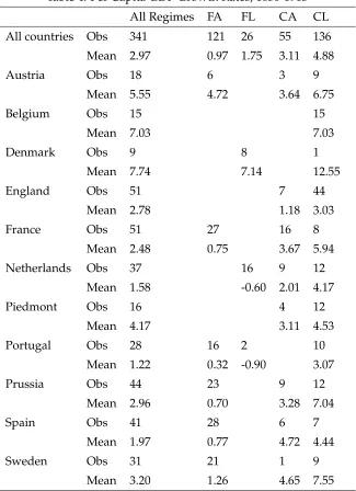
period for fragmented and limited (1.75), centralized and absolutist (3.11), and central-ized and limited (4.88) regimes were high relative to those for fragmented and absolutist ones (0.97).
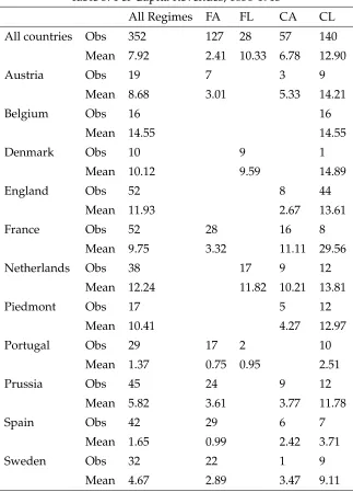
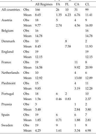
We argue that a key reason why economic outcomes were better under centralized and limited regimes was because states were able to both extract large tax funds and productively use them. Table 5 describes the relationships between political regimes and extractive capacity in terms of per capita revenues from 1650 to 1913. Average per capita revenues in gold grams per five-year period for fragmented and limited (10.33), central-ized and absolutist (6.78), and centralcentral-ized and limited (12.90) regimes were high rela-tive to those for fragmented and absolutist ones (2.41). Similarly, Table 6 describes the relationships between political regimes and productive capacity in terms of per capita non-military spending from 1816 to 1913. Average per capita non-military expenditures in gold grams five-year period for fragmented and limited (6.23), centralized and abso-lutist (6.76), and centralized and limited (11.41) regimes were also high relative to those for fragmented and absolutist ones (1.35).
Table 7 summarizes the 1816-1913 spending data that are disaggregated beyond non-military expenditures. These data are only available for a subset of six sample countries. Furthermore, there are no observations for fragmented and absolutist regimes. Although these limitations prevent us from subjecting the disaggregated spending data to econo-metric analysis, it is still useful to examine the descriptive statistics. Recall from Section 3 that welfare spending by nineteenth-century states was typically low. We focus on two non-military public services that central governments typically provided: infrastructure and education. Average per capita infrastructure and education spending five-year pe-riod for centralized and limited regimes (1.02 and 0.81 gold grams, respectively) was high relative to other regime types. The case study of France in the next subsection further
ex-20Although GDP data from Barro and Urs ´ua (2010) are a potential performance alternative, they are not
amines how disaggregated non-military expenditures varied over political regimes.21
4.2
Case Study of France
The overall trends in Tables 3 to 7 are consistent with our argument that political trans-formations improved economic performance through greater state capacity. These pat-terns also hold for individual countries. To further illustrate the linkages between polit-ical regimes and fiscal and economic outcomes, we now examine France, a core sample country for which long data series over various regime types are available.22
Figure 1 plots French national government revenues from 1650 to 1913. Revenues were low, averaging just more than 3 gold grams per capita, under the fragmented and absolutist regime that lasted through 1789. There was a sharp increase in revenues, which roughly doubled to 10 gold grams per head, in the two decades after fiscal cen-tralization in 1790. Revenues leveled out, but never fell back to pre-1789 levels, in the decades just after the Napoleonic era.23 In the 1840s, they began to increase once more, reaching 18 gold grams per capita by the end of the 1860s. The establishment of a stable centralized and limited regime took place in the aftermath of the Franco-Prussian War (1870-1). This set of events was associated with another jump in revenues, which more
than doubled to nearly 40 gold grams per head by 1913.24
How about expenditures? Figure 2 plots spending on infrastructure and education by the French national government from 1816 to 1913. Infrastructure and education expen-ditures under the centralized and absolutist regime were low, averaging less than 0.43 gold grams per capita, through the late 1820s. However, this spending nearly doubled to 0.82 gold grams per head under the short-lived centralized and limited July regime
(1830-48).25 Napoleon III established authoritarian rule in 1851. During his reign, he
fought five wars.26Although there was an uptick in infrastructure and education
spend-21Although primary school enrollment rates are a potential non-fiscal alternative, enrollment data from
Clemens and Williamson (2004), the most comprehensive historical database that we know of, are not available prior to the 1860s. Nevertheless, the existing data indicate that enrollment rates under centralized and limited regimes were high relative to other regime types.
22Our account follows Dincecco (2011, chs. 3-5 and 8), who also provides sources.
23Furthermore, France never again defaulted on its public debt over the nineteenth century, although it had
done so five times from 1650 to 1789.
24Per capita revenues in gold grams increased by more than 33 times from 1650 to 1913, while per capita
GDP increased by less than four times, indicating that state capacity improvements in France were not simply the result of economic development. Nonetheless, our econometric analysis controls for this factor.
25The vertical lines demarcating this regime in Figures 3 and 4 are dashed to indicate that it was not counted
as limited under our benchmark coding scheme. Also see Section 2.
ing at the start of the 1860s, it was relatively flat, averaging just 1.00 gold gram per capita. With the establishment of a stable centralized and limited regime in 1870-1, there was a rapid jump in infrastructure and education expenditures, which doubled to more than 2 gold grams per head by the start of the 1880s. Infrastructure and education spending continued to increase through 1913, reaching 3.54 gold grams per capita.
To complete this picture, Figure 3 plots the share of infrastructure and education ex-penditures in total exex-penditures for the French national government over the same pe-riod. This share jumped from 5 to 8 percent under the centralized and limited July regime from 1830 to 1848. Under the authoritarianism of Napoleon III, however, it fell to 5 per-cent during the late 1850s and again with the Franco-Prussian War (1870-1). Under the centralized and limited regime established in 1870-1, the share of infrastructure and edu-cation spending reversed course, reaching 8 percent by the start of the 1880s. This share continued to rise, although at a slower rate, through 1913.
Like the descriptive statistics, the case-study evidence for France supports our ar-gument regarding the state capacity benefits of political transformations. Both tax cen-tralization and limited government were associated with greater revenues, and limited government with greater non-military expenditures. Finally, average per capita GDP growth rates per five-year period in France increased from 0.75 under the fragmented and absolutist regime to 3.67 under the centralized and absolutist one, and to 5.94 under the centralized and limited one (Table 4).
4.3
Structural Breaks Tests
To complete this section, we now perform structural breaks tests, which assume no a priori knowledge of major turning points in the fiscal time series. If these tests indicate that political transformations coincided with structural breaks, then we will have fur-ther motivating evidence that the transformations were associated with state capacity improvements. For each sample country, we estimate multiple structural breaks in the fiscal series following Bai and Perron (2003). Our linear regression models include ei-ther a constant or a constant and a country-specific trend as regressors, with all of the coefficients subject to shifts.27 To determine the number of breaks, we use the Bayesian Information Criterion (BIC).
Table 8 reports the 95 percent confidence intervals for the structural break dates.
(1859-61), Battle of Mentana (1867), and Franco-Prussian War (1870-1).
27Both specifications delivered similar results. Varying the trimming parameters did not substantively alter
Panel A displays the results for log per capita revenues from 1650 to 1913, and Panel B the results for log per capita non-military expenditures from 1816 to 1913.28 Our analysis indicates that the structural break confidence intervals encompass the dates of political transformations for the vast majority of sample cases. Given that we use five-year aver-ages, which smooth data fluctuations over time, these results are even more striking. In Panel A for France, for instance, the confidence interval ranging from 1765 to 1790 en-compassed fiscal centralization (1790), while the 1860-1870 interval enen-compassed limited government (1870). In other cases, the dates of political transformations fell just outside of the 95 percent confidence intervals (e.g., limited government in Piedmont in 1848 in Panel B).
Overall, the descriptive statistics, the case study of France, and the structural breaks tests highlight the fiscal and economic impacts of political transformations. To control for the impacts of observable and unobservable factors beyond political regimes, we now perform a full-fledged econometric analysis.
5
Econometric Methodology
We base our benchmark econometric model on the theoretical framework in Section 3, where (1) political regime type affects state extractive and productive capabilities and (2) state capacity in turn affects economic performance. We express this model as the following set of two equations:
logFit =α0+α1CAit−1+α2FLit−1+α3CLit−1+α4′Xit−1+µi+λt+ǫit, (1)
and
∆Yit =β0+β1logFit−1+β2′Xit−1+µi+λt+νit, (2)
wherei=1, . . . ,Ndenotes countries,t=1, . . . ,Tdenotes time,Fitdenotes the extractive
and productive capacity measures as per capita revenues and non-military expenditures,
respectively, ∆Yit denotes economic performance as growth in real log per capita GDP,
CAit−1,FLit−1, andCLit−1are lagged political regime indicators,Xit−1is a lagged vector of controls,µiandλtare country and time fixed effects, andǫitis the error term. We lag
28For this analysis and the subsequent one described in Section 5, we express the state capacity (and
the independent variables, both to reduce the likelihood of simultaneity (Jones, 1995), and because our historical narrative in Section 2 suggests that political transformations, which often took place in chaotic environments, likely required a grace period for full implementation.29 We use clustered standard errors to account for within-country corre-lations.
The key independent variables in Equation 1 are the lagged political regime indica-torsCAit−1,FLit−1, andCLit−1, which take the value 1 for each sample year that a coun-try had a centralized and absolutist (fragmented and limited, centralized and limited) regime and 0 otherwise, with the fragmented and absolutist regimeFAit−1as the bench-mark. These dummies represent a clear, concise, and intuitive way to measure the fiscal impacts of political institutions. Recall from Section 2 that our coding of regimes biases the data against the hypothesis that political transformations improved state capacity.30
The vectorXit−1comprises a set of controls. Military spending was by far the largest component of national budgets through the nineteenth century (Hoffman and Rosen-thal, 1997). Furthermore, Aghion et al. (2012) argue that military rivalry was an impor-tant factor in the historical rise of mass education. To account the impacts of warfare, we include a dummy variable for each year of external conflicts in Europe according to Dincecco (2011). To control for the fiscal impact of internal conflicts, which disrupted tax and spending flows, we include a dummy variable for each year of civil war, coup, or revolution, also from Dincecco (2011). Acemoglu et al. (2005a) argue that Atlantic trade was key to Europe’s early economic success. They use time-invariant characteristics to measure trade potential, which our country fixed effects capture.31 Comin et al. (2010) argue that “old” technology affects long-run development. Our country fixed effects capture their measure of technology adoption in 1500. From 1750 onward, England was the global technological leader. Our country fixed effects also capture country-level dif-ferences in geographical distances to the English border (i.e., the technological frontier). Bockstette et al. (2002) and Putterman and Weil (2010) argue that a long history of state-hood positively influences long-term growth. To control for state antiquity, we include
the measure from Putterman (2007).32 Early technology and state antiquity help to
cap-29We selected the optimal lag length based on the Bayesian Information Criterion (BIC) (Schwarz, 1978).
30As an alternative, we used an ordered specification that coded political regimes from least to most effective
according to Table 3. The results indicated that there were notable state capacity differences between political regimes.
31These are whether the country was an Atlantic trader (England, France, the Netherlands, Portugal, and
Spain), or the Atlantic coastline-to-area ratio. They also account for the aggregate volume of Atlantic trade, which our time fixed effects capture.
nation-ture the impact of human capital accumulation, which Glaeser et al. (2004) argue is an important source of long-run development.
While the previous set of controls applies to Equations 1 and 2 alike, two additional controls are specific to Equation 1. First, since countries at different development stages could have chosen different state capacity levels (e.g., Glaeser et al., 2004), we control for lagged per capita GDP. We also restrict the analysis to the pre-industrial period as a robustness check. Second, our theoretical framework indicates that extractive capacity levels affected productive capacity. We thus control for lagged per capita revenues in the specifications with non-military expenditures as the dependent variable.
Our difference-in-differences approach estimates the impacts of political regimes on state capacity, and of state capacity on economic performance. We also control for time-varying factors and include country-specific time trends. However, the model assump-tions can still be violated in a manner that generates correlaassump-tions between our variables of interest and the error term and biases our results.
One concern is reverse causation. In Equation 1, for instance, it is possible that state capacity improvements preceded political transformations, and that continued improve-ments after transformations reflected underlying capacity trends rather than the impacts of the transformations themselves. However, the historical evidence described in Sec-tion 2 suggests that it is plausible to treat political transformaSec-tions as the result of quasi-random variation or shocks. We also perform placebo tests for which we recode political transformations as a robustness check.
A second concern is omitted variables. For instance, it is likely that the shocks that generated political transformations, and the transformations themselves, had unobserved time-varying, country-specific consequences beyond state capacity improvements that
also affected economic performance.33 Depending on whether the economic impacts of
these consequences were positive or negative, then our results would overestimate or underestimate, respectively, the performance impacts of state capacity.
Since political transformations likely influenced economic performance through a range of channels, we are skeptical of using them to instrument for capacity
improve-state.
33As described in Section 2, there were some cases of incomplete or failed institutional reform. By
ments. However, we are still able to address omitted variable bias in several ways. Be-yond our set of time-variant controls and fixed effects, we include country-specific time trends to account for unobservable factors that changed smoothly but differently across countries. We also test two alternative models to difference-in-differences. The first adds a lagged dependent variable to control for persistent performance impacts. Since OLS estimates are biased in models with lagged dependent variables and country fixed ef-fects, however, we must exclude the fixed effects. The second uses GMM (Blundell and Bond, 1998), enabling us to include country fixed effects while concomitantly accounting for potential simultaneity bias and the (weak) endogeneity of the regressors through the use of internal instruments.34 We present results based on the difference GMM estimator,
which instruments for the lagged dependent variable with differenced past values.35 We
complement the difference specification with forward orthogonal deviations (Arellano and Bover, 1995), which improves estimation efficiency given the unbalanced nature of our panel, and allows us to account for the potential “weak instruments” problem when
outcomes are persistent.36 GMM estimation is based on the assumption that the error
terms are uncorrelated, and, for the case of forward orthogonal deviations, that changes in the instrumenting variables are uncorrelated with the fixed effects. While we recog-nize that these assumptions are strong, Hansen tests of overidentification restrictions and Arellano-Bond autocorrelation tests indicate that our sample satisfies them.
6
Impacts of Political Regimes on State Capacity
6.1
Extractive Capacity
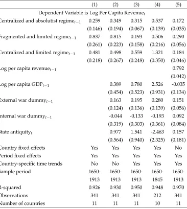
Table 9 presents the results of our estimations for the impacts of political regimes on ex-tractive capacity in terms of per capita revenues from 1650 to 1913 according to Equation 1. Column (1) reports the results for the parsimonious difference-in-differences specifi-cation. Political transformations had significant positive impacts on extractive capacity. The move from the fragmented and absolutist regime to the fragmented and limited one increased per capita revenues by 84 percent over the subsequent five-year period, the
34Although our main GMM specification allows for contemporaneous independent variables, the results are
similar if we lag the independent variables as for OLS.
35As is standard, we use all of the differenced past values as instruments (MaCurdy, 2007). The largeTin
our panel, however, may give rise to the “many instruments” problem. For robustness, we severely restricted the number of instruments to two to five lags. The results were similar. Instrumenting for the key independent variable with differenced past values did not significantly alter the results either.
move to the centralized and absolutist one by 26 percent, and the move to the central-ized and limited one by 48 percent.
Column (2) adds the time-varying controls. The impacts of political transformations on per capita revenues are similar in magnitude and significance as before. Now the revenue impact of the move to the centralized and absolutist regime increases to 35 per-cent. While external conflicts had a positive and sometimes significant revenue impact, internal conflicts typically had a negative but negligible impact. The revenue impact of state antiquity was typically positive but negligible.
Column (3) adds country-specific time trends. The results for the moves to the cen-tralized and absolutist regime and the cencen-tralized and limited one resemble the previous ones. While the move to the fragmented and limited regime remains positive, it is no longer significant. However, its significance is restored in the specifications that follow.
Many political transformations, and in particular the establishment of limited gov-ernment, took place from 1848 onward (Tables 1 and 2). Furthermore, the Industrial Rev-olution took place in continental Europe from 1870 to 1913 (Mokyr, 1998). As a robust-ness check, Column (4) restricts the data to the pre-1848 period. The impacts of political transformations on per capita revenues are all significant. Furthermore, the magnitudes of the moves to the centralized and absolutist regime and the centralized and limited one greatly increase in magnitude. Now the move to the centralized and absolutist regime increased per capita revenues by 54 percent, and the move to the centralized and limited one by 132 percent.
Finally, Column (5) reports the results for the alternative model that adds a lagged dependent variable. The revenue impacts of political transformations are again all sig-nificant. Under standard assumptions, we can view the coefficient magnitudes of our key independent variables in this specification as lower bound estimates (Angrist and Pischke, 2009). These magnitudes remain substantial. Now political transformations are associated with a 17 to 29 percent increase in per capita revenues.37
6.2
Productive Capacity
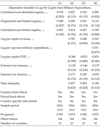
Table 10 reports the sister results for the impacts of political regimes on productive capac-ity in terms of per capita non-military expenditures from 1816 to 1913. Columns (1) to (4) repeat the Table 9 specifications except for the pre-1848 period specification, which is not feasible due to the lack of pre-nineteenth century non-military spending data. Political
37As a further sensitivity test, we excluded sample countries one at a time for our main specifications in
transformations had positive and generally significant impacts on productive capacity. The move from the fragmented and absolutist regime to the fragmented and limited one increased per capita non-military expenditures by 11 to 35 percent over the subsequent five-year period, the move to the centralized and absolutist one by 22 to 58 percent, and the move to the centralized and limited one by 20 to 83 percent. The move to the frag-mented and limited regime is not significant in Columns (1) and (4). However, since there are just 10 observations over two countries for this regime type, we can only ob-tain very imprecise estimates of this parameter. In line with the theoretical predictions, the signs of the conflict variables switch from the previous set of results for per capita revenues. External conflicts had a negative non-military spending impact, while internal conflicts typically had a positive impact. However, the significance of both impacts was negligible. The non-military spending impact of state antiquity was typically positive but negligible.
For robustness, Table 11 presents the results for the impacts of political regimes on
non-productive capacity in terms of per capitamilitaryexpenditures. In stark contrast
with the set of results for non-military spending, the impacts of political transformations on military spending were always negligible. Furthermore, the majority of regime co-efficients were negative. This comparison provides further support for the claim that political transformations had substantial impacts on government spending habits.
In sum, the results described in these two subsections indicate that political transfor-mations had significant positive impacts on state extractive and productive capabilities. These results are robust across a wide variety of specifications, controls, samples, and modeling techniques.
6.3
Placebo Tests
greatly from the previous sets of estimates, by contrast, will lend further credence to our results.
Columns (1) to (4) display the estimates of the impacts of the placebo political regimes on extractive capacity in terms of per capita revenues. Column (1) recodes fiscal central-ization and limited government 15 years prior to the actual years, while Columns (2) to (4) increase the placebos to 25, 35, and 50 years prior, respectively. The results are strik-ing. Placebo political transformations never have a positive and significant impact on per capita revenues. Indeed, all regime coefficients except for one are now negative. The impact of the placebos for the move to the centralized and absolutist regime are always negative and significant, as are the 50-year placebos for all regime types.
Columns (5) to (7) repeat this exercise for the impacts of the placebo political regimes on productive capacity in terms of per capita non-military expenditures for the 15-, 25-, and 35-year placebos25-, respectively (the 50-year placebo is not feasible due to the lack of non-military expenditure data prior to 1815). The results are again striking. With one exception, placebo political transformations never have a significant impact on per capita non-military expenditures. The exception is the 15-year placebo for the move to the centralized and limited regime. However, this impact becomes negative for the 25-and 35-year placebos. The impacts of the 25- 25-and 35-year placebos for the move to the centralized and absolutist regime and the 35-year placebo for the move to the fragmented and limited one are also negative.
Overall, the results of the placebo tests indicate that political transformations were associated with abrupt improvements in state capacity that were not already underway. Given that these transformations likely required a grace period to fully take hold, the short temporal gaps between the actual years of political transformations and their place-bos imply that our test criteria are quite strict.38 Thus, while the placebo results do not allow us to completely exclude the possibility of reverse causation, they markedly en-hance our argument that political transformations had significant positive impacts on state capacity.39
38For instance, the tests in Stasavage (2012) recode the placebo dates of political change (in his case, the
establishment of political autonomy in medieval Europe) 100 years prior to the actual dates.
39As another robustness check, we tested a series of panel probit models for each of the political regime
indicators regressed on lagged per capita revenues and non-military expenditures, as well as on the remaining
predictor variables included in Xit−1. The coefficients for the extractive and productive capacity measures
7
Impacts of State Capacity on Performance
Table 13 presents the results of our estimations for the impacts of state capacity on eco-nomic performance in terms of per capita GDP growth according to Equation 2. Columns (1) to (4) display the estimates of the performance impacts of extractive capacity in terms of per capita revenues. The first three columns reports the results for the difference-in-differences specifications. Improvements in extractive capacity had significant positive impacts on economic performance. A 1 percent increase in per capita revenues led to a 0.384 to 0.833 percentage point increase in the growth rate of per capita GDP over the subsequent five-year period. Given that average growth was 3 percent per five-year pe-riod from 1650 to 1913, this impact is substantial.40
Column (4) reports the results for the lagged dependent variable model. While the performance impact of greater extractive capacity remains positive, it is no longer sig-nificant. However, the GMM equivalent of this specification (to be described ahead), which includes both the lagged dependent variable and country fixed effects, restores the positive and significant impact.
Columns (5) to (7) display the sister estimates of the performance impacts of pro-ductive capacity in terms of per capita non-military expenditures for the difference-in-differences specifications. Productive capacity improvements typically had significant positive impacts on economic performance. The specifications in Columns (5) and (6) indicate that a 1 percent increase in per capita non-military expenditures led to a 1.261 to 3.272 percentage point increase in the growth rate of per capita GDP over the subsequent five-year period. Since average growth was 5 percent per five-year period from 1816 to 1913, this impact is large.41
In the specification with country-specific time trends in Column (7), the performance impact of greater productive capacity is negligible (the sign turns negative). However, this impact is positive and significant in the GMM equivalent of this specification to be described ahead. Furthermore, Column (8) repeats this specification with an alternative productive capacity measure, the share of non-military expenditures in total expendi-tures. The non-military spending share had a positive and significant performance
im-40An alternative interpretation is as follows. Since the move from the fragmented and absolutist regime to
the centralized and limited one led to a roughly 40 percent average per capita revenue increase, our estimates would imply that, holding all else constant, the establishment of an effective state led to a 15 to 33 percentage point increase in the subsequent growth rate of per capita GDP.
41Alternatively, given that the move to the centralized and limited regime led to a roughly 40 percent average
pact: a 1 percent increase in this share led to a 0.109 percentage point increase in the growth rate of per capita GDP over the subsequent five-year period. For further com-parison, Column (9) substitutes per capita military for non-military expenditures and repeats the Column (7) specification. As our theoretical framework predicts, this substi-tution delivers a far worse result. The performance impact of greater military spending is negative and significant: a 1 percent increase in per capita military spending led to a 4.687 percentage point decrease in the growth rate of per capita GDP over the subsequent five-year period. Finally, Column (10) reports the results for the lagged dependent vari-able model. Per capita non-military expenditures again have a positive and significant growth impact.
For robustness, Table 14 presents the results for the performance impacts of state ca-pacity for the GMM model. State caca-pacity improvements had significant positive growth impacts in all specifications except for one. The exception is the specification for extrac-tive capacity in terms of per capita revenues with country-specific time trends in Col-umn (3). While the coefficient on per capita revenues remains positive, it is no longer significant. However, recall that the OLS equivalent of this specification as described previously delivered the positive and significant impact. The specification for produc-tive capacity in terms of per capita non-military expenditures with country-specific time trends in Column (6) is now significant and large: a 1 percent increase in per capita non-military spending led to a 3.272 percentage point increase in the growth rate of per capita GDP per five-year period. The performance impact of the non-military spending share in Column (7) remains significant and doubles in magnitude from OLS. Finally, while the performance impact of greater per capita military spending in Column (8) is no longer significantly negative as it was for OLS, it (in contrast to non-military spending) is still not significantly positive.
Summarizing, the results described in this section indicate that improvements in state extractive and productive capabilities had significant positive impacts on economic per-formance. These impacts are robust to a broad range of specifications, controls, and modeling techniques.
8
Conclusion
abso-lutist. We argue that the establishment of states with modern extractive and productive capabilities had strongly positive performance impacts.
To rigorously develop our claim, we perform a panel regression analysis on a novel database that spans eleven countries and four centuries. Our approach accounts for po-tential biases induced by simultaneity, omitted variables, and unobserved heterogeneity. Placebo tests allow us to further assess the validity of our findings. The results indicate that the performance impacts of state capacity improvements are significant, large, and robust.
Data Appendix
Data for per capita tax revenues from 1650 to 1913 are from Dincecco (2011, appendices A.1, A.2, A.3). See Section 4 for further details.
Data sources for military, infrastructure, and education expenditures per capita are listed ahead. Disaggregated expenditure data in home currencies were converted into gold grams fol-lowing the methodology in Dincecco (2011, appendix A.2). Data for total expenditures and popu-lation are from Dincecco (2011, appendices A.1, A.2) unless otherwise stated. These data use total spending by national governments including debt service and incorporate loan amounts when given. Non-military expenditures per head were computed as per capita total expenditures mi-nus per capita military expenditures.
Austria.Military spending data are from Pammer (2010, Figure 5.1). Infrastructure and education
expenditure data are not available.
Belgium.Military spending data are from Singer (1987). They were downloaded from the
Corre-lates of War website as the National Military Capabilities Dataset, Version 4.0. Infrastructure and education expenditure data are not available.
Denmark. Military spending data are from Singer (1987). They were downloaded from the
Cor-relates of War website as the National Military Capabilities Dataset, Version 4.0. Infrastructure and education expenditure data are not available.
England. Military, infrastructure, and education spending data are from Mitchell (1988, public
finance table 4). To compute military expenditures, spending for the Army and Ordnance and for the Navy were summed. Infrastructure expenditures uses the spending category for Works and Buildings, and education expenditures the category for Education, Art, and Science.
France. Military, infrastructure, and education spending data are from Fontvieille (1976, Tables
CVXI-XXXV). Infrastructure expenditures uses the spending category for Public Works.
Netherlands. Military spending data are from van Zanden (1996, table 4) for 1816-41. Van