Improved tests for spatial correlation

Munich Personal RePEc Archive

Improved tests for spatial correlation

Robinson, Peter M. and Rossi, Francesca

London School of Economics, University of Southampton

22 June 2012

Online at

https://mpra.ub.uni-muenchen.de/41835/

Improved Tests for Spatial Correlation

Peter M. Robinson and Francesca Rossi

London School of Economics and University of Southampton

June 22, 2012

Abstract

We consider testing the null hypothesis of no spatial autocorrelation against the alternative of first order spatial autoregression. A Wald test statistic has good first-order asymptotic properties, but these may not be relevant in small or moderate-sized samples, especially as (depending on properties of the spatial weight matrix) the usual parametric rate of convergence may not be attained. We thus develop tests with more accurate size properties, by means of Edgeworth expansions and the bootstrap. The finite-sample performance of the tests is examined in Monte Carlo simulations.

JEL classifications: C12; C21

1

Introduction

The modelling and analysis of spatially correlated data can pose significant complica-tions and difficulties. Correlation across spatial data is typically a possibility, due to competition, spillovers, aggregation and other circumstances. Such correlation might be anticipated in observable variables or in the unobserved disturbances in an econo-metric model, or both. In, for example, a linear regression model with exogenous regressors, if only the regressors are spatially correlated the usual rules for large sam-ple inference (based on least squares) are unaffected. However, if also the disturbances are spatially correlated then though least squares estimates of the regression coeffi-cients are likely to retain their consistency property, their asymptotic variance matrix reflects the correlation. This matrix needs to be consistently estimated in order to carry out statistical inference, and its estimation (whether parametric or nonparamet-ric) offers greater challenges than when time series data are involved, due to the lack of ordering in spatial data, as well as possible irregular spacing or lack of reliable infor-mation on locations. In addition least squares estimates are rendered asymptotically inefficient by spatial correlation, and developing generalized least squares estimates is similarly beset by ambiguities.

A sensible first step in data analysis is therefore to investigate whether or not there is evidence of spatial correlation, by carrying out a statistical test of the null hypothesis of no spatial correlation. Many such asymptotically valid tests are poten-tially available, so one might focus on ones that are likely to have reasonable power against anticipated alternatives. This requires specifying a parametric model for the spatial correlation. A widely applicable and popular model is the (first-order) spatial autoregression (SAR). For simplicity we stress the case of zero mean observable data; we shall also allow in some of the paper for an unknown intercept but our work can also be extended to test for lack of spatial correlation in unobservable disturbances in more general models, such as regressions. Given then×1 vector of observations

y= (y1, ..., yn) ′

, the prime denoting transposition, the SAR model is

y=λW y+ǫ, (1.1)

where ǫ = (ǫ1, ..., ǫn) ′

consists of unobservable, uncorrelated random variables with zero mean and unknown varianceσ2, λ is an unknown scalar, and W is an n×n

user-specified “weight” matrix, having (i, j)-th element wij, where wii = 0 for all

iand (in order to identify λ) normalization restrictions satisfied. Such restrictions imply that in general each elementwij changes with nas nincreases, implying that

W,and thusy,form triangular arrays (i.e. W =Wn= (wijn), y=yn= (yin)) but we

suppress reference to thensubscript. The elementwijcan be regarded as a (scaled)

the applicability of the model beyond situations when they are known, and entailing simpler modelling than is typically possible when one attempts to incorporate locations of irregularly spaced geographical observations.

The null hypothesis of interest is

H0:λ= 0, (1.2)

whence theyi are uncorrelated (and homoscedastic). An obvious statistic for testing

(1.2) is the Wald statistic based on the least squares estimate ˆλofλ, which is given by

ˆ

λ= y

′

W y

y′_W′_{W y}. (1.3)

Due to the dependence between right-hand side observables and disturbances in (1.1), ˆ

λ is inconsistent for λ, as discussed by Lee (2002). However, ˆλ does converge in probability to zero when λ = 0, so a test statistic for (1.2) based on ˆλ might be expected to be asymptotically valid. In particular, under (1.1), (1.2) and regularity conditions a central limit theorem for independent non-identically distributed random variables gives

h

tr W W′

/

tr W2+W W′ 1/2iˆλ→dN(0,1). (1.4)

Since the square-bracketed norming factor can be directly computed, asymptotically valid Wald tests against one-sided (λ >0 orλ <0) or two-sided (λ6= 0) hypotheses are readily carried out.

The accuracy of such tests is dependent on the magnitude ofn, and the normal approximation might not be expected to be good for smallishn. Moreover, under conditions described later and as shown by Lee (2004) for the Gaussian maximum likelihood estimate of λ, the rate of convergence in (1.4) can be less than the usual parametric rate n1/2_{, depending on the assumptions imposed on W as n increases.}

In particular ifwij =O(1/h) is imposed, where the positive sequence h= hn can

increase no faster thann, the rate is (n/h)1/2_{, which increases more slowly thann}1/2

unlesshremains bounded. This outcome renders the usefulness of the Wald test based on (1.4) more dubious than in standard parametric situations.

our tests in Monte Carlo simulations, comparing also with the simple uncorrected test and tests based on the bootstrap, which (see e.g. Singh (1981) or Hall (1992a)) might be expected to achieve our Edgeworth correction. Proofs are left to an appendix.

Our results are fairly straightforwardly extendable to situations in whichy rep-resents unobservable disturbances in regression models, and in which the intercept model we consider is extended to include explanatory variables, but as the topic of higher-order approximations in spatial econometrics is relatively new, we focus here on the most basic, classical settings.

2

Edgeworth expansions for the least squares

es-timate

The present section develops a (third-order) formal Edgeworth expansion for ˆλ in (1.3) under the null hypothesis of no spatial correlation (1.2). We introduce first some further definitions and assumptions.

Assumption 1The ǫi are independent normal random variables with mean zero

and unknown variance σ2_.

Normality is an unnecessarily strong condition for the first-order result (1.4), but it provides some motivation for stressing a quadratic form objective function and is familiar in higher order asymptotic theory. Edgeworth expansions and resulting test statistics are otherwise complicated by the presence of cumulants ofǫi. Assumption 1

implies that under (1.2) theyi are spatially independent.

For a real matrixA, let||A||be the spectral norm ofA(i.e. the square root of the largest eigenvalue ofA′

A) and let||A||∞be the maximum absolute row sums norm of

A(i.e. ||A||∞= max i

P

j

|aij|, in whichaijis the (i, j)th element ofAandiandjvary

respectively across all rows and columns ofA). LetKbe a finite generic constant.

Assumption 2

(i) For all n, wii= 0,i= 1, ..., n.

(ii) For all sufficiently largen,W is uniformly bounded in row and column sums in absolute value, i.e. ||W||∞+||W

′

||∞≤K

(iii) For all sufficiently large n, uniformly in i, j = 1, ..., n, wij = O(1/h), where

h=hnis a positive sequence bounded away from zero for allnsuch that h/n→0

as n→ ∞.

to keep spatial correlation manageable. Commonly in practical applications W is symmetric with non-negative elements and row normalized, such that Σnj=1wij = 1

for alli, in which case Assumption 2(ii) is automatically satisfied. Part (iii) covers two cases which have rather different implications for our results: eitherhis bounded (when in (1.4) ˆλenjoys a parametricn1/2_{rate of convergence), orhis divergent (when}

ˆ

λhas a slower than parametric, (n/h)1/2, rate). By way of illustration consider (see Case (1991)),

Wn=Ir⊗Bm, Bm= 1

m−1(lml

′

m−Im), (2.1)

where Is is the s×s identity matrix, lm is the m×1 vector of 1’s, and⊗ denotes

Kronecher product. HereW is symmetric with non-negative elements and row nor-malized,n=mr. Parts (i) and (ii) of Assumption 2 are satisfied, andh∼m, where “∼” throughout indicates that the ratio of left and right sides converges to a finite, nonzero constant. Thus in the boundedhcase onlyr→ ∞asn→ ∞, whereas in the divergenthcasem→ ∞andr→ ∞.

Now define

tij= h

ntr(W

i

W′j), i≥0, j≥0, i+j≥1, (2.2)

t= h

ntr((W W

′

)2). (2.3)

Under Assumption 2 all tij in (2.2) and t are O(1) (because, for any real A such

that||A||∞ ≤K, we havetr(AW) = O(n/h) ). To ensure the leading terms of the

expansion in the theorem below are well defined, we introduce

Assumption 3

lim

n→∞

h

n(t20+t11)>0. (2.4)

By the Cauchy inequality, Assumption 3 implies lim_n→∞ht11/n > 0, and the two conditions are equivalent when W is symmetric or when its elements are all non-negative. Assumption 3 is automatically satisfied under (2.1). It follows from Assumptions 2 and 3 that in (1.4) the norming factor

tr(W W′) (tr(W2_{) +W W}′₎1/2 =

t11

(t20+t11)1/2

n

h

1/2

∼n

h

1/2

. (2.5)

Now define

a= t11

(t20+t11)1/2, b=

t21

(t20+t11)1/2_t11, c=

2t30+ 6t21

(t20+t11)3/2, (2.6)

d= t

t2 11

, e= 12(t31+t22) (t20+t11)t11, f=

6t40+ 24t31+ 6t22+ 12t

(t20+t11)2 , g=

1

and

U(ζ) = 2bζ2−c

6H2(ζ), (2.8)

V(ζ) =1

6(e−6bc)ζH2(ζ)−(d−6b

2_)ζ3₋ 1

24f H3(ζ) + 1 3bcζ

2_H3(ζ)−2b2_ζ5_{, (2.9)}

whereHj(ζ) is thejth Hermite polynomial, such that

H2(ζ) =ζ2−1 H3(ζ) =ζ3−3ζ. (2.10)

ThusU(ζ) is an even, generally non-homogeneous, quadratic function ofζ, whileV(ζ) is an odd, generally non-homogeneous, polynomial inζ of degree 5.

Write Φ(ζ) =P r(Z ≤ζ) for a standard normal random variableZ, and φ(ζ) for the probability density function (pdf) ofZ. LetF(ζ) =P(n/h)1/2aλˆ≤ζ.

Theorem 1Let (1.1) and Assumptions 1-3 hold. UnderH0 in (1.2), for any realζ, F(ζ)admits the third order formal Edgeworth expansion

F(ζ) = Φ(ζ) +U(ζ)φ(ζ)

h n

1/2

+V(ζ)φ(ζ)h

n+O

h n

3/2!

, (2.11)

where

U(ζ) =O(1), V(ζ) =O(1), (2.12)

asn→ ∞.

Generally,U(ζ) andV(ζ) are non-zero, whence there are leading correction terms of exact orders (h/n)1/2 _{andh/n, and both terms are known functions ofζ.}

A corresponding result to Theorem 1 is available for the pure SAR model with unknown intercept, i.e.

y=µl+λW y+ǫ, (2.13)

whereµis an unknown scalar andl=ln. The least squares estimate ofλin (2.13) is

˜

λ= y

′

W′

P y

y′_W′_{P W y}, (2.14)

whereP =In−l(l′l)−1l′. Under (1.2), the same kind of regularity conditions and the

additional

Assumption 4For all n,Σn

j=1wij= 1,i= 1, ..., n,

˜

that of ˆλand, in particular, ˜λ converges to the true value at the standardn1/2 _rate

whetherhis bounded or divergent asn→ ∞. Since the main goal of this paper is to provide refined tests when the rate of convergence might be slower than the parametric raten1/2, the case of model (2.13) whenW is not row-normalized is not considered here.

Define

˜

U(ζ) =U(ζ) +g1/2 (2.15)

and

˜

V(ζ) =V(ζ) +

g

2(1 +p) + 2bg

1/2₋g4

2

ζ−2bg2ζ3+cg

1/2

6 H3(ζ), (2.16)

where

p=l′W W′l/n. (2.17)

(WhenW is symmetric Assumption 4 impliesp= 1). Let ˜F(ζ) =P((n/h)1/2_aλ˜_≤ζ).

Theorem 2Let (2.13) and Assumptions 1-4 hold. UnderH0 in (1.2), for any realζ,

˜

F(ζ)admits the third order formal Edgeworth expansion

˜

F(ζ) = Φ(ζ) + ˜U(ζ)φ(ζ)

h n

1/2

+ ˜V(ζ)φ(ζ)h

n+O

h n

3/2!

, (2.18)

where

˜

U(ζ) =O(1), V˜(ζ) =O(1), (2.19)

asn→ ∞.

The second- and third-order correction terms are again generally non-zero, and of orders (h/n)1/2 _{and h/nrespectively. Notice that ˜U(ζ) > U(ζ), so the second-order}

approximate distribution function (df) of ˜λis greater than that of ˆλ. The Edgeworth approximation in (2.18) is unaffected byµ(and the approximations in both (2.11) and (2.18) are unaffected by σ2_{). Consequently results can be similarly obtained when}

there is a more general linear regression component than in (2.13), at least when regressors are non-stochastic or strictly exogenous. Indeed, similar techniques will yield approximations with respect to the model y−µl = λW(y−µl) +ǫ, or more general linear regression models with SAR disturbances.

Finally, it is worth stressing that Theorems 1 and 2 hold not only under Assump-tion 1, but also for the class of spherically symmetric distributed disturbances (e.g. Hillier (2001) or Forchini (2002)). Specifically, let w =ǫ(ǫ′

ǫ)−1/2_{, where ǫ satisfies}

Assumption 1. Thus, w is uniformly distributed on the unit sphere in ℜn_{. It can}

be shown that the distributions of both ǫ′

W ǫ/ǫ′

W′

W ǫ and ǫ′

W′

P ǫ/ǫ′

W′

P W ǫ are the same as those ofw′

W w/w′

W′

W wandw′

W′

P w/w′

W′

spherically symmetric distribution for ǫ, since any random vector within such class would implywbeing uniformly distributed on the unit sphere inℜn.

3

Improved tests for no spatial correlation

We consider first tests of the null hypothesis (1.2) against the alternative

H1: λ >0 (3.1)

in the no-intercept model (1.1).

Forα∈(0,1) (for exampleα= 0.05 orα= 0.01) define the normal critical value

zα such that 1−α= Φ(zα). Writeq= (n/h)1/2aˆλ. On the basis of (1.4) a test that

rejects (1.2) against (3.1) when

q > zα (3.2)

has approximate sizeα. Theorem 1 readily yields more accurate tests that are simple to calculate because the coefficients ofU(ζ) andV(ζ) are known,W being chosen by the practitioner.

Define the exact critical valuewα such that 1−α=F(wα), so a test that rejects

whenq > wαhas exact sizeα. Also introduce the Edgeworth corrected critical value

uα=zα−

_h

n

1/2

U(zα). (3.3)

Corollary 1Let (1.1) and Assumptions 1-3 hold. UnderH0 in (1.2), asn→ ∞

wα=zα+O

h n

1/2!

(3.4)

=uα+O

h n

. (3.5)

Corollary 1 follows follows immediately from Theorem 1. From Corollary 1, the test that rejects (1.2) against (3.1) when

q > uα (3.6)

is more accurate than (3.2). Of course when the alternative of interest isλ <0, the same conclusion can be drawn for the tests which reject whenq < −zα, q < −uα,

respectively.

statistic that can be compared withzα. Introduce the polynomial

G(ζ) =ζ+

h n

1/2

U(ζ) +h

n

1 3

2b−c 6

2

ζ3. (3.7)

which has known coefficients (see Yanagihara et al. (2005)). SinceG(ζ) has derivative (1 +ζ(2b−c/6)(h/n)1/2₎2_{>0, it is monotonically increasing. ThusF(ζ) =P(G(q)≤} G(ζ)) and we invert the expansion in Theorem 1 to obtain

Corollary 2Let (1.1) and Assumptions 1-3 hold. UnderH0, asn→ ∞

P(G(q)> zα) =α+O

h n

. (3.8)

Thus the test that rejects when

G(q)> zα (3.9)

has size that differs fromαby smaller order than the size of (3.2).

Still more accurate tests can be deduced from Theorem 1 by employing also the third-order correction factorV(ζ), but the above tests have the advantage of simplicity. TheV term, however, is especially relevant in deriving improved tests against the two-sided alternative hypothesis

H0: λ6= 0. (3.10)

BecauseU(ζ) is an even function it follows from Theorem 1 that

P(|q| ≤ζ) = 2Φ(ζ)−1 + 2h

nV(ζ) +O

h n

3/2!

. (3.11)

Thence define the Edgeworth-corrected critical value for a two-sided test,

vα/2=zα/2− n

hV(zα/2), (3.12)

noting that the approximate size-α two-sided test based on (1.4) rejectsH0 against (3.10) when

|q|> zα/2. (3.13)

Corollary 3Let (1.1) and Assumptions 1-3 hold. UnderH0, asn→ ∞

sα/2=zα/2+O

h n

(3.14)

=vα/2+O

h n

3/2!

. (3.15)

Thus rejecting (1.2) against (3.10) when

|q|> vα/2 (3.16)

rather than (3.13) reduces the error toO((h/n)3/2_{). In fact, Theorem 1 can be}

estab-lished to fourth-order, with fourth-order term that is even inζ, and errorO((h/n)2_),

so the error in (3.15) can be improved toO((h/n)2).

As with the one-sided alternative (3.1), a corrected test statistic that can be com-pared withzα/2 can be derived from Theorem 1. Define (Yanagihara et al. (2005))

L(ζ) =ζ+h

nV(ζ)

+

_h

n

2 ₁

4

L21ζ+ L2

2ζ5

5 +

L2 3ζ9

9 +

2 3L1L2ζ

3₊2

5L1L3ζ

5₊2

7L2L3ζ

7_{, (3.17)}

whereL1=−1

6(e−6bc)+ 1 8f,L2=

1

2(e−6bc)−3(d−6b 2₎₋1

8f−3bcandL3= 5 3bc−10b

2_,

so L(ζ) is a degree-7 polynomial in ζ with known coefficients. It is readily checked thatV(ζ) has derivativeL1+L2ζ2+L3ζ4, whereL(ζ) has derivative (1 + (h/n)(L1+

L2ζ2_+L3ζ4_)/2)2 _{>0 and is thus monotonically increasing. Therefore, from (3.11),}

we obtain

Corollary 4Let (1.1) and Assumptions 1-3 hold. UnderH0, asn→ ∞

P(L(|q|)> zα/2) =α+O

h n

3/2!

. (3.18)

The transformation in (3.17) and Corollary 4 follow from (3.11) using a minor modification of Theorem 2 of Yanagihara et al. (2005). From the latter result, we conclude that the test that rejectsH0 against (3.10) when

L(|q|)> zα/2 (3.19)

has size which is closer toαthan (3.13).

Improved tests can be similarly derived from Theorem 2 for the intercept model in (2.13). We first consider tests ofH0 in (1.2) against (3.1). Let ˜q = (n/h)1/2_aλ˜.

approximate levelαwhen

˜

q > zα. (3.20)

Define the exact and Edgeworth-corrected critical values ˜wα, such that 1−α= ˜F( ˜wα),

and ˜uα=zα−U˜(zα)(h/n)1/2=uα−g1/2(h/n)1/2, respectively.

Similarly to Corollaries 1 and 2, from Theorem 2 we deduce

Corollary 5Let (2.13) and Assumptions 1-4 hold. UnderH0 in (1.2), asn→ ∞

˜

wα=zα+O

h n

1/2!

(3.21)

= ˜uα+O

_h

n

. (3.22)

Notice that ˜uα< uα for anyα, so that the second-order corrected critical value is

lower for the intercept model. Let

˜

G(ζ) =ζ+

_h

n

1/2

˜

U(ζ) +h

n

1 3

2b−c 6

2

ζ3=G(ζ) +

_h

n

1/2

g1/2. (3.23)

Corollary 6Let (2.13) and Assumptions 1-4 hold. UnderH0 in (1.2), asn→ ∞

P( ˜G(˜q)> zα) =α+O

h n

. (3.24)

Thus, tests that reject (1.2) against (3.1) when either

˜

q >u˜α (3.25)

or

˜

G(˜q)> zα, (3.26)

are more accurate than (3.20).

Also, from Theorem 2 improved tests of (1.2) against (3.10) can be deduced. From (2.18), since ˜U(ζ) is an even function we obtain,

P(|q˜| ≤ζ) = 2Φ(ζ)−1 + 2h

nV˜(ζ) +O

h n

3/2!

. (3.27)

Define ˜sα/2 such that P(|q˜| ≤ s˜α/2) = 1−α and ˜vα/2 = zα/2−(n/h) ˜V(zα/2). A

standard, approximate sizeα, two-sided test rejects (1.2) against (3.10) when

From (3.27) we deduce

Corollary 7Let (2.13) and Assumptions 1-4 hold. UnderH0, asn→ ∞

˜

sα/2=zα/2+O

h n

(3.29)

= ˜vα/2+O

h n

3/2!

. (3.30)

Finally, define

˜

L(ζ) =ζ+h

nV˜(ζ)

+

h n

2

1 4

˜

L21ζ+

˜

L22ζ5

5 +

L23ζ9

9 +

2 3L1˜ L2ζ˜

3₊2

5L1L3ζ˜

5₊2

7L2L3ζ˜

7_{, (3.31)}

where ˜L1=L1+g₂(1 +p) + 2bg1/2₋g4

2 −

cg1/2

2 ,L2˜ =L2−6bg

1/2₊cg1/2

2 .

Corollary 8Let (2.13) and Assumptions 1-4 hold. UnderH0, asn→ ∞

P( ˜L(|q˜|)> zα/2) =α+O

h n

3/2!

. (3.32)

From Corollaries 7 and 8, we conclude that the tests that rejectH0against (3.10) when either

|q˜|>˜vα/2 (3.33)

or

˜

L(|q˜|)> zα/2 (3.34)

have sizes closer toαthan that obtained from (3.28).

Before concluding this section we should acknowledge that the distribution func-tions under (1.2) and Assumption 1 of bothqand ˜qcan also be evaluated numerically using the procedure introduced by Imhof (1961) (for implementation details see e.g. Lu and King (2002)). Exact critical values can then be numerically calculated. However, Imhof-type of implementations heavily rely on numerical solutions of highly non-linear equations and therefore might not be not fully reliable.

4

Bootstrap correction and simulation results

e.g. Singh (1981)). For the no-intercept model (1.1) the bootstrap test is as follows (e.g Paparoditis and Politis (2005)). We construct 199n×1 vectorsǫ∗

j, whose elements

are independently generated asN(0,σˆ2_{),j = 1, ....,199.The bootstrap test statistic}

isq∗

j= (n/h)1/2aǫ ∗′

j W ′

ǫ∗ j/ǫ

∗′

j W ′

W ǫ∗

j,j= 1, ...,199, its (1−α)th percentile beingu ∗ α

which solvesP199

j=11(q

∗ j≤u

∗

α)/199≤1−α,where 1(.) indicates the indicator function.

We reject (1.2) against the one-sided alternative (3.1) when

q > u∗α. (4.1)

Defining the (1−α)th percentile of|q∗

j|as the valuev ∗

αsolvingP199j=11(|q

∗ j| ≤v

∗ α)/199≤

1−α,we reject (1.2) against the two-sided alternative (3.10) if

|q|> vα∗. (4.2)

For the intercept model (2.13) we define ˜q∗

j = (n/h)1/2a˜ǫ ∗′

j W ′

Pǫ˜∗ j/ǫ˜

∗′

j W ′

P W˜ǫ∗ j,

j = 1, ...,199, where the components of each ˜ǫ∗

j are independently generated from

N(0,˜σ2_{) with ˜σ}2 _=y′

P y/n. The (1−α)th quantiles of ˜q∗ j and|q˜

∗ j|, ˜u

∗ α and ˜v

∗ α, solve

P199

j=11(˜q

∗ j ≤u˜

∗

α)/199≤1−α,andP199j=11(|q˜

∗ j| ≤˜v

∗

α)/199≤1−α, respectively. We

reject (1.2) against (3.1) or (3.10) when

˜

q >u˜∗α (4.3)

or

|q˜|>˜vα∗, (4.4)

respectively.

In the simulations we setσ2 _{= 1 in Assumption 1,µ= 2 in (2.13) and chooseW}

as in (2.1), for variousmandr. Recalling that orders of magnitudes in Theorems 1 and 2 are affected by whetherhdiverges or remains bounded asn→ ∞, we represent both cases by different choices ofm∼h. We choose (m, r) = (8,5), (12,8), (18,11), (28,14), i.e. n = 40, 96, 198, 392, to represent “divergent” h, and (m, r) = (5,8), (5,20), (5,40), (5,80), i.e. n= 40, 100, 200, 400 to represent “bounded”h. For each of these combinations we compute ˆλand ˜λfrom the same realization ofǫacross 1000 replications. In all testsα= 0.05.

Empirical sizes are displayed in Tables 1-8, in which “normal”, “Edgeworth”, “transformation” and “bootstrap” refer respectively to tests using the standard normal approximation, Edgeworth-corrected critical values, Edgeworth-corrected test statis-tic and bootstrap cristatis-tical values, and the respective abbreviations N, E, T, B will be extensively used in the text.

(Tables 1 and 2 about here)

model (1.1), whenhis respectively “divergent” and “bounded”. Test N is drastically under-sized for eachnin both tables. The sizes for E are somewhat better, and improve asnincreases, in particular for “divergent”hthe discrepancy between empirical and nominal sizes is 18.2% lower relative to N, on average across sample size, while as n

increases this discrepancy decreases by about 0.7% for N, but by 9.5% for E. Both T and B perform well for alln. Indeed, on average, whenhis “divergent” empirical sizes for T and B are 80.4% and 85.4%, respectively, closer to 0.05 than those for N, with a similar pattern in Table 2. Tables 1 and 2 are consistent with Theorem 1 in whichF converges to Φ at raten1/2 _{when his bounded, but only at rate (n/h)}1/2

whenhis divergent. Indeed, whenhis “bounded”, on average the difference between empirical and nominal size decreases by 6.8% asnincreases for N, while this difference only decreases by 0.7% in case h is “divergent”. Also, from Table 2, the average improvements offered by E, T and B over N are about 41%, 88% and 84%, respectively. Overall, T and B perform best.

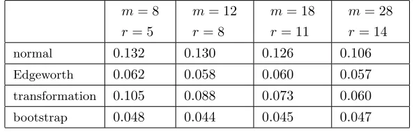
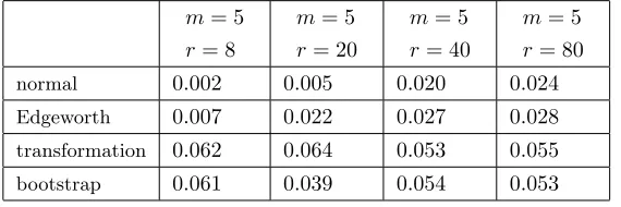
(Tables 3 and 4 about here)

Tables 3 and 4 cover two-sided tests for the no-intercept model (1.1), namely (3.13), (3.16), (3.19) and (4.2). Again, N is very poor, though contrary to the one-sided test case the problem is now over-sizing, and E, T and B all offer notable improvements. Indeed, whenh is “divergent” the difference between empirical and nominal sizes is reduced respectively on average across sample sizes by 87.4%, 59% and 94% for E, T and B relative to N, and by 86%, 59% and 95% whenhis “bounded”. In the tables B seems overall most accurate, followed by E.

(Tables 5 and 6 about here)

Tables 5 and 6 contain results for one-sided tests for the intercept model (2.13), the N, E, T and B tests being given in (3.20), (3.25), (3.26) and (4.3). The pattern is similar to that displayed in Tables 1 and 2. For “divergent”h, on average across sample sizes, empirical sizes for E, T and B are 12%, 65% and 89% closer to 5% than ones for N, with figures of 21.7%, 78.7% and 81% for “bounded”h. Overall, B performs best for “divergent”h, but it is difficult to choose between B and T whenh

is “bounded”.

(Tables 7 and 8 about here)

(Figures 1 and 2 about here)

To illustrate the effect of the transformationsG(.) and ˜G(.) used in Section 3, in Figures 1 and 2 we plot the histograms with 100 bins ofq and G(q) (Figure 1) and of ˜q and ˜G(˜q) (Figure 2) obtained from 1000 replications when m= 28 andr = 14. Both figures suggest that the densities ofqand ˜q are very skewed to the left and that most of the skewness is removed by the transformations, as in Hall (1992b).

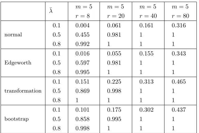
(Tables 9-12 about here)

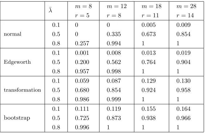
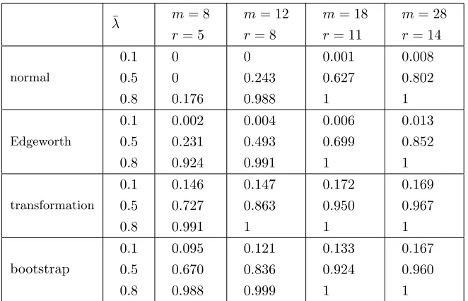
In Tables 9-12 we assess power against a fixed alternative, i.e.

H1:λ= ¯λ >0. (4.5)

Tables 9 and 10 display the empirical power of one-sided tests in the no-intercept model (1.1) whenhis “divergent” and “bounded” respectively, while Tables 11 and 12 correspondingly contain results for the intercept model (2.13). These are non-size-corrected tests. Exept for the smallest sample size when h is “divergent”, even N performs well for the largest ¯λ= 0.8, as do all other tests in all settings. N also does comparably well to E, T and B whenh is bounded and ¯λ = 0.5. But overall N is outperformed by the other tests, with T and B offering the greatest power.

A remark on consistency of standard and corrected tests is desirable. As previously mentioned, ˆλand ˜λ are inconsistent whenλis non-zero. Therefore, in caseplimλ <ˆ λ (> λ) as n → ∞for λ >0 (λ < 0), it might be that under H1, plimˆλ= 0 as

n → ∞, with the same possibilities for ˜λ. Then the standard and corrected tests would be inconsistent. For the special case ofW in (2.1), the following theorem shows that the direction of inconsistency follows the sign ofλ.

Theorem 3

(i) Let model (1.1) hold. Under Assumption 1 and (2.1),plim

n→∞

(ˆλ−λ)is finite and has the same sign asλ.

(ii) Let model (2.13) hold. Under Assumption 1 and (2.1), plim

n→∞

(˜λ−λ) is finite and has the same sign asλ.

The proof is in the Appendix. Assumption 1 could be relaxed here, but is retained for algebraic simplicity. Under (1.1), asn→ ∞ plimλ > λˆ (< λ) as n→ ∞ when

λ >0 (λ <0) and hence, P(q > zα|H1) →1, P(q > uα|H1) → 1 and P(G(q) >

zα|H1) → 1. Similarly under (2.13), P(˜q > zα|H1) → 1, P(˜q > u˜α|H1) → 1 and

P( ˜G(˜q)> zα|H1)→1 as n→ ∞. The direction of inconsistency could be computed

Appendix

Proof of Theorem 1

Under H0, ˆλ = ǫ′

W′

ǫ/ǫ′

W′

W ǫ and thus P(ˆλ ≤ x) = P(ς ≤ 0), where ς =

ǫ′(C+C′)ǫ/2,C =W′−xW′W andxis any real number. We proceed much as in, e.g., Phillips (1977). Under Assumption 1, the characteristic function (cf) ofςis

E(eit2ǫ′(C+C′)ǫ) = 1

(2π)n/2_σn

Z

ℜn

eit2ξ′(C+C′)ξe−

ξ′ξ

2σ2_dξ

= 1

(2π)n/2_σn

Z

ℜn

e−2σ12ξ′(I−itσ 2

(C+C′_))ξ

dξ

=det(I−itσ2(C+C′))−1/2=

n

Y

j=1

(1−itσ2ηj)

−1/2_{, (A.1)}

where theηjare eigenvalues ofC+C′anddet(A) denotes the determinant of a generic

square matrixA. From (A.1) the cumulant generating function (cgf) ofς is

ψ(t) =−1 2

n

X

j=1

ln(1−itσ2ηj) =

1 2

n

X

j=1

∞

X

s=1

(itσ2_η

j)s

s

=1 2

∞

X

s=1

(itσ2₎s

s

n

X

j=1 ηsj=

1 2

∞

X

s=1

(itσ2₎s

s tr((C+C

′

)s). (A.2)

Denoting byκsthes−th cumulant ofς, from (A.2)

κ1=σ2tr(C), (A.3)

κ2= σ

4

2 tr((C+C

′

)2), (A.4)

κs=

σ2s_s!

2

tr((C+C′

)s₎

s , s >2. (A.5)

Letςc= (ς−κ1)/κ12/2. The cgf ofςcis

ψc(t) =−1 2t

2

+

∞

X

s=3 κcs(it)s

s! , (A.6)

where

κcs=

κs

so the cf ofςc _is

E(eitςc) =e−12t 2 exp{ ∞ X s=3 κc

s(it)s

s! }

=e−12t 2

{1 +

∞

X

s=3 κc

s(it)s

s! + 1 2!( ∞ X s=3 κc

s(it)s

s! )

2₊ 1

3!(

∞

X

s=3 κc

s(it)s

s! )

3_+...}

=e−1₂t2

{1 +κ

c

3(it)3

3! +

κc4(it)4

4! +

κc5(it)5

5! +{

κc6

6! + (κc3)2

(3!)2}(it)

6_+...}.

(A.8)

Thus by Fourier inversion, formally

P(ςc≤z) =

z

Z

−∞

φ(z)dz+κ

c 3 3! z Z −∞

H3(z)φ(z)dz+κ

c 4 4! z Z −∞

H4(z)φ(z)dz+.... . (A.9)

Collecting the above results,

P(ˆλ≤x) =P(ς≤0) =P(ςcκ₂1/2+κ1≤0) =P(ςc≤ −κc1)

= Φ(−κc1)− κc

3

3!Φ

(3)_(−κc

1) + κc

4

4!Φ

(4)_(−κ′

1) +... . (A.10)

From (A.3), (A.4) and (A.7),

κc1=

tr(C) (1

2tr((C+C

′₎2₎₎1/2. (A.11)

The numerator ofκc

1 is

tr(W)−xtr(W W′) =−xtr(W W′) =−n

hxt11, (A.12)

while its denominator is

(1

2tr(C+C

′

)2)1/2= (tr(W2) +tr(W W′)−4xtr(W2W′) + 2x2tr((W W′)2))1/2.

=n

h

1/2

t20+t11−4xt21+ 2x2t1/2

. (A.13)

Thus

κc1=

−xt11(n/h)1/2

(t20+t11−4xt21+ 2x2_t)1/2 =

−xt11(n/h)1/2

(t20+t11)1/2₍₁₋4xt21−2x2t

(t20+t11) )

1/2. (A.14)

Choose

x=

h n

1/2

(t20+t11)1/2 t11 ζ= (

h n)

1/2

whereawas defined in (2.6). By Taylor expansion

κc1=−ζ

1−4xt21−2x

2_t

(t20+t11)

−1/2

=−ζ−2

_h

n

1/2 _t21

t11(t20+t11)1/2ζ 2 +h n t t2 11

ζ3−6h

n

t21

(t20+t11)1/2_t11

2

ζ3+O

h n

3/2!

=−ζ−2

h n

1/2

bζ2+h

ndζ 3₋₆h

nb 2_ζ3_+O

h n

3/2!

, (A.16)

wherebanddwere defined in (2.6) and (2.7). Then by Taylor expansion and using

(−d/dx)jΦ(x) =−Hj−1(x)φ(x), (A.17)

we have

Φ(−κc1) = Φ ζ+ 2

h n

1/2

bζ2−h

ndζ 3_{+ 6}h

nb 2_ζ3_+O

h n

3/2!!

= Φ(ζ) + 2

_h

n

1/2

bζ2−h

ndζ 3_{+ 6}h

nb 2_ζ3

!

φ(ζ) + 2h

nb

2_ζ4_Φ(2)_{(ζ) +O} h n

3/2!

= Φ(ζ) + 2

h n

1/2

bζ2φ(ζ) + h

n −dζ

3_+b2_(6ζ3_−2ζ4_H1(ζ))

φ(ζ) +O

h n

3/2!

= Φ(ζ) + 2

h n

1/2

bζ2φ(ζ) + h

n −dζ

3_+b2_(6ζ3_−2ζ5₎

φ(ζ) +O

h n

3/2!

.

(A.18)

Similarly,

Φ(3)(−κc1) = Φ(3)(ζ) + 2

h h

1/2

bζ2Φ(4)(ζ) +O

h n

= H2(ζ)−2

_h

h

1/2

bζ2H3(ζ)

!

φ(ζ) +O

_h

n

. (A.19)

From (A.5), (A.7),

κc3=

tr((C+C′

)3) (1

2tr((C+C

′₎2₎₎3/2.

By standard algebra, forxdefined in (A.15),

1

2tr((C+C

′

)2) = n

h t20+t11−4

_h

n

1/2 _(t20+t11)1/2_t21 t11 ζ+O

_h

n

!

=n

h(t20+t11)−4

n

h

1/2(t20+t11)1/2t21

tr((C+C′)3) = n

h 2t30+ 6t21−12

h n

1/2

(t20+t11)1/2_(t31+t22) t11 ζ+O

h n

!

= n

h(2t30+ 6t21)−12

n

h

1/2 (t20+t11)1/2(t31+t22)

t11 ζ+O(1)

(A.21)

and thus

κc3=

n

h(2t30+ 6t21)−12 n h

1/2

(t20+t11)1/2(t31+t22)t−1

11ζ+O(1)

n h

3/2

(t20+t11)3/2₁₋₄ h n

1/2

t21t−1

11(t20+t11)−1/2ζ+O hn

3/2

=

h n

1/2

2t30+ 6t21

(t20+t11)3/2 −12 h n

t31+t22

t11(t20+t11)ζ+O

h n

3/2!!

× 1 + 6

h n

1/2

t21

t11(t20+t11)1/2ζ+O

h n ! = h n

1/2

2t30+ 6t21

(t20+t11)3/2 −12 h n

t31+t22 t11(t20+t11)ζ+

h n

6(2t30+ 6t21)t21

(t20+t11)2_t11 ζ+O

h n

3/2!

=

h n

1/2

c−h

n(e−6bc)ζ+O

h n

3/2!

, (A.22)

whereb,cande were defined in (2.6) and (2.7). Similarly,

3tr((C+C′)4) =n

h(6t40+ 24t31+ 12t+ 6t22) +O

n

h

1/2

(A.23)

and thus

κc4= h n

6t40+ 24t31+ 12t+ 6t22

(t20+t11)2 +O

h n

3/2!

= h

nf+O

h n

3/2!

, (A.24)

wherefwas defined in (2.7).

Substituting (A.15), (A.18), (A.19), (A.22) and (A.24) in (A.10) and rearranging using (2.8) and (2.9) completes the proof.

Proof of Theorem 2

UnderH0 and by Assumption 2(i), ˆλ=ǫ′

W′

P ǫ/ǫ′

W′

P W ǫ. Proceeding as before,

P(˜λ ≤ x) = P(ς ≤0), which can be written as the right side of (A.10), with ς =

ǫ′

(C+C′

)ǫ/2 and

C=W′P(I−xW). (A.25)

1, and so is not described in detail. From (A.25), (2.2) and (2.17),

κ1=σ2tr(C) =−σ21 +xtr(W′

W)−x

n(l

′

W W′

l)=−σ21 +xn ht11−xp

.

(A.26) Similarly, since

l′WiW′jl=O(n) for all i≥0, j≥0, (A.27)

κ2=σ

4

2tr((C+C

′

)2)

=σ4

tr(W2) +tr(W′W)−1−1

nl

′

W′W l−4x(tr(W W′W) +O(1)) + 2x2(tr((W′W)2) +O(1))

=σ4n

h(t20+t11)−1−p−4x

n

ht21+O(1)

+ 2x2n

ht+O(1)

. (A.28)

Proceeding as in the proof of Theorem 1, the first centred cumulant ofς is

κc1=

−xn

ht11−1 +xp n

h(t20+t11)

1/2 1−

1 +p+ 4x n

ht21+O(1)

−2x2 n

ht+O(1)

n

h(t20+t11)

!−1/2

.

(A.29)

Settingxas in (A.15) and by Taylor expansion,

κc1=−

ζ+ (h/n)

1/2

(t20+t11)1/2 − h n

p t11ζ

× 1 +

_h

n

1/2 _2t21

t11(t20+t11)1/2ζ+ h n

₁

2(t20+t11)+ 1 2

p t20+t11−

t t2 11

ζ2+ 6t

2 21 t2

11(t20+t11) ζ2 ! +O h n

3/2!

=− ζ+

h n

1/2

g1/2−h

n p t11ζ ! 1 + h n

1/2

2bζ+h

n

g

2+

g

2p−dζ

2_{+ 6b}2_ζ2

!

+O

_h

n

3/2!

=−ζ−

h n

1/2

(2bζ2+g1/2)−h

n

g

2ζ+

g

2pζ−dζ

3_{+ 6b}2_ζ3_{+ 2bg}1/2_ζ

+O

h n

3/2!

,

(A.30)

withb, d,g and pdefined in (2.6), (2.7) and (2.17). Similarly, by standard algebra and using (A.27),

tr((C+C′)3) = n

h(2t30+ 6t21)−12

n

h

1/2(t20+t11)1/2(t31+t22)

agreeing with the corresponding formula in the proof of Theorem 1, so that the third centred cumulant ofς,κc3, is (A.22), whereas the fourth centred cumulant ofς,κc4, is

again (A.24). Next,

Φ(−κc1) = Φ(ζ) +

h n

1/2

(2bζ2+g1/2)φ(ζ) + h

n

g

2ζ+

g

2pζ−dζ

3_{+ 6b}2_ζ3_{+ 2bg}1/2_ζ

φ(ζ)

+1 2(2bζ

2

+g1/2)2Φ(2)(ζ) +O

h n

3/2!

= Φ(ζ) +

h n

1/2

(2bζ+g1/2)φ(ζ)

+h

n

_g

2ζ+

g

2pζ−dζ

3_{+ 6b}2_ζ3_{+ 2bg}1/2_ζ−1

2(2bζ

2_+g1/2₎2_H1(ζ)φ(ζ)

+O

h n

3/2!

(A.32)

and

Φ(3)(−κc1) = Φ(3)(ζ) +

h h

1/2

(2bζ2+g1/2)Φ(4)(ζ) +O

h n

= H2(ζ)−

_h

h

1/2

(2bζ2+g1/2)H3(ζ)

!

φ(ζ) +O

_h

n

. (A.33)

Substituting (A.15), (A.22), (A.24), (A.32) and (A.33) in the right side of (A.10) complete the proof.

Proof of Theorem 3

(i)From (1.1),y=S−1(λ)ǫ, whereS(x) =In−xW. Under (2.1),S−1(λ) exists for

anyλ∈(−1,1) and

S−1(λ) =

∞

X

i=0

(λW)i. (A.34)

From (A.34)S−1_{(λ) is symmetric,S}−1_{(λ)W =W S}−1_{(λ) and||S}−1_(λ)||

∞≤K.

For anyλ∈(−1,1),

ˆ

λ−λ= y

′

W ǫ y′_W2_y =

hǫ′

S−1_{(λ)W ǫ/n}

hǫ′_S−1_(λ)W2_S−1_(λ)ǫ/n. (A.35)

Asn→ ∞, the numerator of the RHS of (A.35) converges in probability to

lim(h/n)σ2tr(S−1_{(λ)W) since (h/n)(ǫ}′

S−1_{(λ)W ǫ−σ}2_tr(S−1_{(λ)W))→ 0 in second}

probability tolim(h/n)σ2_tr((S−1_(λ)W)2_{). Thus}

ˆ

λ−λ→p

lim

n→∞ h ntr(S

−1_(λ)W)

lim

n→∞ h ntr((S

−1_(λ)W)2₎. (A.36)

First we show that the RHS of (A.36) is finite. Since||S−1_(λ)||

∞≤K,

(h/n)tr(S−1_{(λ)W) = O(1).The denominator in the RHS of (A.36) is non-negative}

and, by (A.34), (h/n)tr((S−1_(λ)W)2_{)∼(h/n)tr(W}2_{),which is non-zero under (2.1).}

Hence, the RHS of (A.36) is finite and its sign depends on its numerator. From (2.1) and (A.34),

tr(S−1_{(λ)W) =tr(}

∞

X

i=0

λitr(Wi+1)) =r

∞

X

i=0

λitr(Bim+1). (A.37)

SinceBmhas one eigenvalue equal to 1 and the other (m−1) equal to−1/(m−1),

tr(Bmi+1) = 1 + (m−1)

−1

m−1

i+1

(A.38)

and hence, since|λ|<1,

tr(S−1(λ)W) =r

∞

X

i=0 λi 1−

₋₁

m−1

i!

= r

1−λ− r

1 + λ m−1

= λ

1−λ rm m−1 +λ.

(A.39) By substitutingh=m−1 andn=mrinto (A.39),

h ntr(S

−1_{(λ)W) =}m−1 mr

λ

1−λ rm m−1 +λ =

λ

1−λ

m−1

m−1 +λ, (A.40)

which, for allλ∈(−1,1), has the same sign ofλ, whethermis divergent or bounded, for allm >1.

(ii)Under (2.13),

˜

λ−λ= y

′

W P ǫ y′_{W P W y} =

hǫ′

S−1_{(λ)W P ǫ/n}

hǫ′_S−1_{(λ)W P W S}−1_(λ)ǫ/n, (A.41)

wherey=S−1_{(λ)(µl+ǫ) and since from (A.34) l}′

S−1_{(λ)W P =l}′

S−1_(λ)′

W′

P = 0. Thus, similarly to (A.36),

˜

λ−λ→p

lim

n→∞ h ntr(S

−1_{(λ)W P)}

lim

n→∞ h ntr((S

−1_(λ)W)2_P). (A.42)

The result in (ii) follows from the proof of part (i), after observing that, asn→ ∞,

=lim(h/n)tr((S−1_(λ)W)2_{) +o(1).}

References

Case, A.C. (1991). Spatial Patterns in Household Demand. Econometrica,59, 953-65.

Forchini, G. (2002). The Exact Cumulative Distribution Function of a Ratio of Quadratic Forms in Normal Variables, with Applications to the AR(1) Model.

Econometric Theory18, 823-52.

Hall, P. (1992a). The Bootstrap and Edgeworth Expansion. Springer-Verlag. Hall, P. (1992b). On the Removal of Skewness by Transformation. Journal of the Royal Statistical Society. Series B 54, 221-28.

Hillier, G. (2001). The Density of a Quadratic Form in a Vector Uniformly Distributed on then−Sphere.Econometric Theory 17, 1-28.

Imhof, J.P. (1961). Computing the Distribution of Quadratic Forms in Normal Variables. Biometrika,48, 266-83.

Kelejian, H.H. and I.R. Prucha (1998). A Generalized Spatial Two-Stages Least Squares Procedure for Estimating a Spatial Autoregressive Model with Autore-gressive Disturbances. Journal of Real Estate Finance and Economics 17, 99-121.

Lee, L.F. (2002). Consistency and Efficiency of Least Squares Estimation for Mixed Regressive, Spatial Autoregressive Models. Econometric theory 18, 252-77.

Lee, L.F. (2004). Asymptotic Distribution of Quasi-Maximum Likelihood Esti-mates for Spatial Autoregressive Models. Econometrica72, 1899-1925. Lu, Z.H. and M.L.King (2002). Improving the Numerical Techniques for Com-puting the Accumulated Distribution of a Quadratic Form in Normal Variables.

Econometric Reviews 21, 149-65.

Paparoditis, E. and D.N. Politis (2005). Bootstrap Hypothesis Testing in Re-gression Models. Statistics & Probability Letters 74, 356-65.

Phillips, P.C.B. (1977). Approximations to Some Finite Sample Distributions Associated with a First-Order Stochastic Difference Equation. Econometrica,

45, 463-85.

m= 8

r= 5

m= 12

r= 8

m= 18

r= 11

m= 28

r= 14

normal 0 0 0.001 0.001

Edgeworth 0.004 0.008 0.010 0.016

transformation 0.036 0.038 0.040 0.047

bootstrap 0.039 0.061 0.053 0.054

Table 1: Empirical sizes (nominalα= 0.05) of tests ofH0 (1.2) againstH1 (3.1) in

no-intercept model (1.1) whenhis “divergent”.

m= 5

r= 8

m= 5

r= 20

m= 5

r= 40

m= 5

r= 80

normal 0.001 0.001 0.001 0.011

Edgeworth 0.001 0.025 0.028 0.034

transformation 0.042 0.045 0.043 0.052

bootstrap 0.043 0.040 0.057 0.055

Table 2: Empirical sizes (nominalα= 0.05) of tests ofH0 (1.2) againstH1 (3.1) in

no-intercept model (1.1) whenhis “bounded”.

m= 8

r= 5

m= 12

r= 8

m= 18

r= 11

m= 28

r= 14

normal 0.132 0.130 0.126 0.106

Edgeworth 0.062 0.058 0.060 0.057

transformation 0.105 0.088 0.073 0.060

bootstrap 0.048 0.044 0.045 0.047

Table 3: Empirical sizes (nominal α = 0.05) of tests of H0 (1.2) against H1 (3.10) in

m= 5

r= 8

m= 5

r= 20

m= 5

r= 40

m= 5

r= 80

normal 0.096 0.078 0.068 0.061

Edgeworth 0.062 0.051 0.049 0.052

transformation 0.055 0.025 0.042 0.052

bootstrap 0.049 0.047 0.051 0.050

Table 4: Empirical sizes (nominal α = 0.05) of tests of H0 (1.2) against H1 (3.10) in

no-intercept model (1.1) whenhis “bounded”.

m= 8

r= 5

m= 12

r= 8

m= 18

r= 11

m= 28

r= 14

normal 0 0 0.001 0.001

Edgeworth 0.003 0.005 0.007 0.010

transformation 0.076 0.068 0.064 0.061

bootstrap 0.040 0.048 0.047 0.046

Table 5: Empirical sizes (nominalα= 0.05) of tests ofH0(1.2) againstH1(3.1) in intercept

model (2.13) whenhis “divergent”.

m= 5

r= 8

m= 5

r= 20

m= 5

r= 40

m= 5

r= 80

normal 0.002 0.005 0.020 0.024

Edgeworth 0.007 0.022 0.027 0.028

transformation 0.062 0.064 0.053 0.055

bootstrap 0.061 0.039 0.054 0.053

Table 6: Empirical sizes (nominalα= 0.05) of tests ofH0(1.2) againstH1(3.1) in intercept

m= 8

r= 5

m= 12

r= 8

m= 18

r= 11

m= 28

r= 14

normal 0.281 0.187 0.170 0.148

Edgeworth 0.127 0.123 0.104 0.084

transformation 0.220 0.168 0.140 0.107

bootstrap 0.080 0.070 0.062 0.062

Table 7: Empirical sizes (nominalα= 0.05) of tests ofH0(1.2) againstH1(3.10) in intercept

model (2.13) whenhis “divergent”.

m= 5

r= 8

m= 5

r= 20

m= 5

r= 40

m= 5

r= 80

normal 0.156 0.082 0.063 0.062

Edgeworth 0.103 0.068 0.047 0.048

transformation 0.112 0.065 0.052 0.053

bootstrap 0.042 0.058 0.061 0.040

Table 8: Empirical sizes (nominalα= 0.05) of tests ofH0(1.2) againstH1(3.10) in intercept

model (2.13) whenhis “bounded”.

¯

λ m= 8

r= 5

m= 12

r= 8

m= 18

r= 11

m= 28

r= 14

normal

0.1

0.5

0.8 0

0

0.257 0

0.335

0.994

0.005

0.673

1

0.009

0.854

1

Edgeworth

0.1

0.5

0.8

0.001

0.200

0.957

0.008

0.562

0.998

0.013

0.764

1

0.019

0.904

1

transformation

0.1

0.5

0.8

0.059

0.680

0.986

0.087

0.854

0.999

0.129

0.924

1

0.130

0.958

1

bootstrap

0.1

0.5

0.8

0.111

0.725

0.996

0.119

0.873

1

0.155

0.938

1

0.164

0.966

1

Table 9: Empirical powers of tests ofH0 (1.2) againstH1(4.5), with nominal sizeα= 0.05

¯

λ m= 5

r= 8

m= 5

r= 20

m= 5

r= 40

m= 5

r= 80

normal

0.1

0.5

0.8

0.010

0.551

0.999

0.083

0.988

1

0.187

1

1

0.363

1

1

Edgeworth

0.1

0.5

0.8

0.016

0.676

1

0.095

0.992

1

0.200

1

1

0.375

1

1

transformation

0.1

0.5

0.8

0.122

0.858

1

0.172

0.993

1

0.280

1

1

0.420

1

1

bootstrap

0.1

0.5

0.8

0.139

0.888

1

0.203

0.992

1

0.296

1

1

0.451

1

1

Table 10: Empirical powers of tests ofH0(1.2) againstH1(4.5), with nominal sizeα= 0.05

in no-intercept model (1.1) whenhis “bounded”.

¯

λ m= 8

r= 5

m= 12

r= 8

m= 18

r= 11

m= 28

r= 14

normal

0.1

0.5

0.8 0

0

0.176 0

0.243

0.988

0.001

0.627

1

0.008

0.802

1

Edgeworth

0.1

0.5

0.8

0.002

0.231

0.924

0.004

0.493

0.991

0.006

0.699

1

0.013

0.852

1

transformation

0.1

0.5

0.8

0.146

0.727

0.991

0.147

0.863

1

0.172

0.950

1

0.169

0.967

1

bootstrap

0.1

0.5

0.8

0.095

0.670

0.988

0.121

0.836

0.999

0.133

0.924

1

0.167

0.960

1

Table 11: Empirical powers of tests ofH0(1.2) againstH1(4.5), with nominal sizeα= 0.05

¯

λ m= 5

r= 8

m= 5

r= 20

m= 5

r= 40

m= 5

r= 80

normal

0.1

0.5

0.8

0.004

0.455

0.992

0.061

0.981

1

0.161

1

1

0.316

1

1

Edgeworth

0.1

0.5

0.8

0.016

0.597

0.995

0.055

0.981

1

0.155

1

1

0.343

1

1

transformation

0.1

0.5

0.8

0.151

0.869

1

0.225

0.998

1

0.313

1

1

0.465

1

1

bootstrap

0.1

0.5

0.8

0.101

0.858

0.998

0.175

0.995

1

0.302

1

1

0.437

1

1

Table 12: Empirical powers of tests ofH0(1.2) againstH1(4.5), with nominal sizeα= 0.05

Figure 1: Histograms of q (left picture) andG(q) (right picture) for 1000 replications,

m= 28,r= 14

−12 −10 −8 −6 −4 −2 0 2

0 10 20 30 40 50 60

−20 −15 −10 −5 0 5

0 10 20 30 40 50 60 70 80 90

Figure 2: Histograms of ˜q (left picture) and ˜G(˜q) (right picture) for 1000 replications,