Munich Personal RePEc Archive
Growth Accelerations: The Role of
Government Expenditures and Revenues
Parekh, Saahil and Pandey, Manish
IIT Kharagpur, University of Winnipeg
August 2012
Online at
https://mpra.ub.uni-muenchen.de/66343/
1
Growth Accelerations: The Role of Government
Expenditures and Revenues
Saahil Parekh and Manish Pandey
Working Paper
This working paper is available for download at:
2
GROWTH ACCELERATIONS: THE ROLE OF GOVERNMENT EXPENDITURES AND
REVENUES
Saahil Parekh
1Indian Institute of Technology Kharagpur
saahil.parekh@gmail.com
Manish Pandey
University of Winnipeg
m.pandey@uwinnipeg.ca
August 10, 2012
Abstract
Using episodes of growth spells, we attempt to resolve the issue of endogeneity by examining differences in fiscal policies before and after the start of the spell. In doing so, we seek to answer the question of whether governments change fiscal policies in response to growth accelerations or whether such changes happen prior to start of growth spells. We use statistically significant growth spells identified by Berg et al. (2011) for our analysis. We find a positive long run trend growth for aggregate ratios of government expenditures and revenues to GDP. However, we find no evidence that the growth of the variables in the pre-period or the post-period differed from their long run trend growth rate.
1 Corresponding author: Saahil Parekh, Department of Humanities and Social Sciences, Indian Institute of Technology
3
1. Introduction
Research in the field of growth economics has a major role to play in terms of supporting the needs of the policy practitioner. Economic growth and its determinants form one of the cornerstones of policy making. However, in his review of the World Bank’s report on Economic Growth in the 1990s, Rodrik (2006) states that there is little evidence that macroeconomic policies, price distortions, financial policies and trade openness have had effects on economic growth. As two extreme examples, he states that countries in sub-Saharan Africa had failed to take off in the 1990s despite significant changes in political and external environments and significant foreign aid. On the other hand, countries like India and China managed to reduce the number of people living under poverty through unconventional policies. Rodrik argues that policy makers need to have a ‘different strokes for different folks’ approach while charting out useful policies intended towards bringing economic growth and that we cannot use a rigid set of policies for everyone.
Recent research in growth economics has seen new endeavours aimed at a better understanding of the determinants of growth in GDP per capita. The focus has shifted to analyzing short periods of growth spurts. Easterly et al. (1993) point out that growth tends to unstable and that very few countries have experienced a constant high growth rate. Typically, countries show phases of growth, stagnation and decline for periods of varying length (Pritchett, 2000). With so much instability in growth rates of a country in terms of both the average level and variance across countries, using explanations of the long run growth rates for policy building can prove to be very misleading. Given these features of economic growth, Pritchett (2000) argues that analysis of the episodes of growth accelerations holds more promise than long term growth.
In particular, for developing countries, given the volatility in growth of GDP per capita, the question of what causes episodes of growth acceleration becomes even more important. Thus if there has been, say, a significant upturn in the growth trend for a country, it would be imperative to analyze what was happening in the country during that time (or a few years prior to the upturn) to understand how to sustain the phenomenon. An analysis using long run growth regressions will miss out on the most interesting variations in data (Hausmann et al., 2005).
Hausmann et al. (2005) were the first to identify turning points in the growth trends of countries and analyze its correlates and predictors. However, they conclude that growth accelerations tend to be highly unpredictable and that most instances of economic reform do not produce growth accelerations. More recently, Jerzmanovski (2006), Jones and Olken (2008) and Berg et al. (2011) also analyze the determinants of growth accelerations.
While a number of determinants of growth accelerations have been examined, the role of government fiscal policies has not received much attention. We address this issue by examining whether there were differences in fiscal policies between countries that had episodes of growth accelerations from those that did not. In doing so, we provide a way of testing the predictions of endogenous growth models that changes in taxation and expenditure will lead to differences in growth rates (Barro, 1990).2
Using data for 22 OECD countries, Kneller et al. (2001) test the predictions of endogenous growth models by examining the relationship between fiscal policies and growth. They divide government expenditures into productive and unproductive, and revenues into distortionary and non-distortionary and find a positive relationship between growth and productive expenditures after controlling for the level of distortionary and non-distortionary taxation. Their findings support the predictions of endogenous growth models. However, their approach does not fully address the issue of endogeneity between fiscal variables and growth rates.
2 The endogenous models of Barro (1990) and King and Rebelo (1990) differ from the conventional neoclassical models in
4
Using episodes of growth spells, we attempt to resolve the issue of endogeneity by examining differences in fiscal policies before and after the start of the spell.3 In doing so, we seek to answer the question of whether governments
change fiscal policies in response to growth accelerations or whether such changes happen prior to start of growth spells. Finding evidence for the former would suggest that growth leads to changes on fiscal policies, while the latter would indicate some evidence in favour of a role for fiscal policies in explaining growth spells.
We analyze difference in the trends of government expenditures and revenues relative to GDP at both aggregated and disaggregated levels between countries that experience growth spells and those that do not. Given that there may not be an overall change in expenditures but changes in composition of government expenditures, we also examine differences in trends in expenditure on functional categories as shares of total expenditures. The trend change in composition of expenditures is important because at a disaggregated level, it allows us to determine changes in allocation across functional categories by the government and thus could provide further insights into role of changes in fiscal policies in explaining growth spells.
We use statistically significant growth spells identified by Berg et al. (2011) for our analysis. Controlling for country specific fixed effects, we examine whether the time trends for government expenditures 10 years before (pre-period) and 10 years after (post-(pre-period) the start of a growth spell differ for countries that experienced a growth spell from the long run average trend for all countries. We start at the aggregate level and then disaggregate expenditures into productive and unproductive and revenues into distortionary and non-distortionary using the definitions in Kneller et al. (2001).4
We find a positive long run trend growth for aggregate ratios of government expenditures and revenues to GDP. However, we find no evidence that the growth of the variables in the pre-period or the post-period differed from their long run trend growth rate. When we divide aggregate expenditures into productive and unproductive components, while the long run trend growth of the ratio of productive expenditures to GDP is negative, the ratio of unproductive expenditures to GDP does not change over time. Similar to the results for aggregate expenditures, we find no evidence that the growth rate of the ratios in the pre- or the post-period differ from their long run trend growth rate. When we divide aggregate revenues into distortionary and non-distortionary taxes, we find a positive long run trend growth in the ratio of non-distortionary taxes to GDP while the ratio of distortionary taxes to GDP does not change over time. We find no evidence that growth rate of the ratios differ from their long run trend in the pre- or the post-periods.
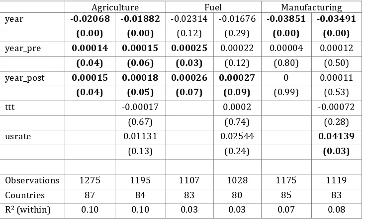
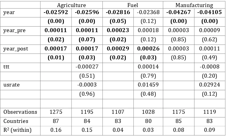
Upon further disaggregation of productive and unproductive expenditures, the results for the various functional groups of productive expenditures are similar to the aggregate results. Among the various functional groups of unproductive expenditures, we find that the growth rate of ratio of government expenditures on provision of goods and services in the agriculture sector to GDP in the pre- and the post-periods were higher than the long run trend. Similar results hold when we consider the ratio of expenditure on provision of goods and services in the agriculture sector to total expenditures. This leads us to conclude that government expenditures in this sector before and after the start of the growth spell were higher than the long run average growth rates for expenditures.
The rest of the paper is organized as follows. Section 2 describes the data we use for our analysis and defines the key variables. Section 3 discusses the fixed effects estimation method that we use for our analysis. The findings are presented and discussed in Section 4. Section 5 provides a brief conclusion.
2. Data
Data on government expenditures and revenues is obtained from the Government Financial Statistics (GFS) dataset provided by the International Monetary Fund (IMF) and complied by William Easterly. It provides aggregate as well as disaggregated data for government expenditures and revenues as a percentage of GDP for about 120 countries
3 A growth spell is a period that starts with a statistical up-break in growth of GDP per capita and is sustained for a period of
8 years. See Section 2 for more details on how growth spells are identified.
4 Productive expenditures are defined as those that add to future productive capacity. Taxes that affect choices of firms or
5
for the period ranging from 1972 to 2000.5 Government expenditure is disaggregated by functional categories and data
is available for main revenue sources.
To examine whether government expenditure and revenue patterns differed between countries that had growth spells and countries that did not, we merge the GFS data with the Berg et al. (2011) computed timing of growth spells as well as data used for their analysis. Berg et al. define growth spells as the time period between growth acceleration and deceleration. Their methodology for determining the spell period is mentioned below:
Period begins with a statistical upbreak followed by a period of atleast 2% average growth GDP per capita.
Period ends with a statistical downbreak followed by a period of less than 2% average growth or with the
end of the sample.
A break is a statistically significant break in the trend growth of GDP per capita. Berg et al. (2011) use a variant of the Bai and Perron (1998) method to test for multiple structural breaks in the trend. The location of potential breaks is decided by minimizing the sum of squared residuals between actual data and the average growth rate before and after the break. They use a minimum interstitiary period between two breaks so that the algorithm does not identify unwanted spurious breaks. They provide for 2 such interstitiary periods, 8 and 5 years. We use the breaks generated using the 8 year period for our analysis.
The merged dataset is an unbalanced panel with information on 87 countries for the period 1972-2000. Given the timing of the start of growth spell obtained from the Berg et al. data, we construct a pre-spell and post-spell period for each growth spell. Pre-spell is a 10 year period before the start of a spell while post-spell is a 10 year period after the start of the spell and includes the year of the start of the spell. We define the 20 year period (10 year pre and the 10 year post) around the start of a growth spell as the adjustment period.
Of the 87 countries in the merged dataset, 23 countries had growth spells during or in a ten period year before 1972.6 Table 1 provides average values for government expenditures to GDP ratio (G/Y), government revenues to GDP
ratio (Revenue/Y), deficit to GDP ratio and average annual growth of per capita GDP (Growth), for all countries, countries with no growth spells and countries with growth spells. The average ratios of government expenditures and government revenues to GDP were similar for countries with growth spells and those with no spells. The average deficit to GDP ratio was lower for countries that had growth spells. The average of the growth rate over the period was higher for countries with no spells (1.80%) relative to countries that had spells (1.62%).
Table 2 provides the averages for the non-adjustment, adjustment, pre- and post-period for countries that had growth spells. Both the ratio of expenditures and revenues to GDP were higher during the adjustment period relative to the non-adjustment period. The ratio being higher in the pre-spell than the post-spell period was the reason for the higher ratio during the adjustment period. However, the deficit to GDP ratio was lower during the adjustment period. Further, average growth rate of GDP per capita was higher in the non-adjustment period than the adjustment period. This was again due to the lower growth rates in the pre-spell period. Such differences suggest that governments of growth spell countries may have undertaken changes in expenditures during the adjustment period. We examine such differences in the next Section.
We also examine differences in the composition of expenditures between countries with growth spells and countries with no spells. The average values of the share of expenditure for the eight functional categories we use for our analysis are presented in Table 3. The eight categories account for 84% of the total government expenditures. The
5 See Easterly (2001) for further details. The data has been posted on the World Bank website as part of the Global
Development Network Growth Database and was downloaded using the following url:
http://econ.worldbank.org/WBSITE/EXTERNAL/EXTDEC/EXTRESEARCH/0,,contentMDK:20701055~pagePK:6421482 5~piPK:64214943~theSitePK:469382,00.html
6
functional categories with the highest expenditure shares were social security and services accounting for about 40% of the total expenditures.7
3. Method of analysis
We are interested in those up-breaks which lead to a growth spell. We analyze the trend around the year when the up-break happens. If the up-break happens at time t, say, then we analyze whether there is a significant change in trend from the long run trend for all countries for periods [t-10, t-1] and [t, t+9], which are pre–spell and post-spell periods, respectively.
We start with ratios of aggregate government expenditures and revenues to GDP and move towards disaggregated expenditures and revenues. For classification of expenditures and revenues, we use the definitions of expenditures and revenues provided by Kneller et al. (2001), with a few modifications. The definitions are as follows:
Productive expenditures – Expenditures on public, defence, education, housing, health and transport
and communication sectors
Unproductive expenditures – Expenditures on social security, recreation and culture and towards (non
productive) consumption of goods and services
Distortionary revenues – Income tax
Non-distortionary revenues – Goods and service tax
The following regression equation is employed to examine the trends in country i at time t:
= + ∗ + ∗ ∗ + ∗ ∗ + +
where is intercept
, , are the coefficients of time and measure growth rates is country specific error term
is the random error term
We perform a fixed effects regression on the panel data to account for variation across countries. is the long run growth rate of the dependent variable for all the countries, which we interpret as the average growth rate across all countries during the period of examination. The variable is a dummy variable which takes value 1 (0 otherwise) for the period [t-10, t-1]. Hence the coefficient provides the difference in growth rate of y during those 10
years before a growth spell from the long run average growth rate. The variable takes value 1 (0 otherwise) for period [t, t+9]. The coefficient provides the difference in growth rate of y for the 10 years after the start of a spell
from the long run average growth rate.
4. Findings
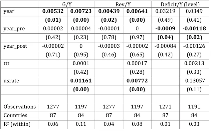
We find a positive and statistically significant long run trend growth in the ratios of government expenditures and revenues to GDP across all countries (refer Table 4). In other words, we find evidence that government size relative to GDP across all countries was increasing over time. However, for countries that experienced growth spells, we fail to find any evidence of a difference in the trend growth in the pre- or the post-period from the long run average rate. The results of the trend growth in the ratio of deficit to GDP are different. Although the long run trend growth for this variable is not statistically significant, we do find significant evidence of a negative trend growth in the pre-period for countries that experienced growth spells.
Next, we divide expenditures into productive and unproductive. These results are summarized in Table 5. We find that the long run trend in growth rate of the ratio of productive expenditures to GDP is negative. This result holds even in the trend of productive expenditures relative to total expenditures. We do not find any evidence of the trends in the pre and post periods being different from the long run average rate. For unproductive expenditures, we find a
7 Services are defined as the amount of government expenditure on economic goods and services provided for consumption.
7
positive long run trend growth in the ratio of unproductive expenditures to GDP but the result is significant only after controlling for terms of trade and U.S. interest rates. However, we do not find any trend when we use unproductive expenditures relative to total expenditures as the dependent variable. Similar to the results of productive expenditures, we find that the pre- or post-period trends are no different from the long run trend.
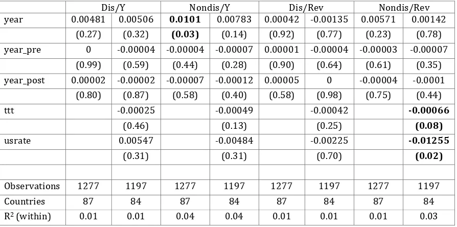
Table 6 provides the results of distortionary and non-distortionary taxes. We do not find any long run trend either in the ratio of distortionary taxes to GDP or distortionary taxes relative to total revenues. Also, we find that the trends in pre- and post-period for countries that saw growth accelerations are no different from the long run trend. The results are similar for non-distortionary taxes, only that we find a positive trend in the long run average rate for the ratio of non-distortionary taxes to GDP. But this result is not robust as the trend becomes insignificant when we add controls for terms of trade and U.S. interest rate.
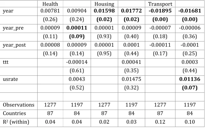
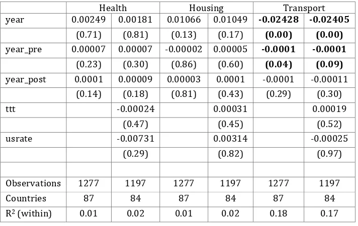
Tables 7a and 7b summarize the results for the ratios of various functional groups of productive expenditures to GDP. Tables 8a and 8b summarize the results relative to total expenditure. We find negative trend growth in the long run rates across all countries for expenditures on public, defence and transport and communication sectors. While we do not find any difference from the long run in the pre- or post-period trend growth rates for public and defence sectors, we do find evidence that the growth rate of the ratio of expenditure on transport and communication to total expenditures during the pre period was lower than the long run average for countries that experienced growth spells. In other words, we find evidence that the share of expenditure on transport and communication was falling at a faster rate than the long run rate before the start of growth acceleration.
8
Table 1: Data Summary: Averages
N G/Y Revenue/Y Deficit/Y Growth (%) All Countries 1277 29.03 27.32 -3.06 1.72 No growth spell Countries 717 30.54 28.69 -3.21 1.80 Growth spell countries 560 27.10 25.56 -2.88 1.62
Table 2: Countries with Growth Spells: Averages
Period N G/Y Revenue/Y Deficit/Y Growth Non-Adjustment 304 26.00 24.28 -3.10 1.77 Adjustment 256 28.41 27.09 -2.63 1.43 Pre-spell 143 29.54 28.18 -2.59 -0.91 Post-spell 125 26.89 25.85 -2.50 4.20
Table 3: Functional Categories of Government Expenditures: Averages
N Relative to GDP Relative to Expenditure Public 1277 2.81 10.42
[image:9.595.119.479.473.697.2]Defence 1277 2.92 10.60 Education 1277 3.43 12.37 Health 1277 2.06 6.97 Housing 1277 0.90 3.12 Social Security 1277 6.60 20.48 Recreation & Cultural 1277 0.40 1.35 Services 1277 5.12 18.62
Table 4: Government expenditure, revenue and deficit in terms of GDP
G/Y Rev/Y Deficit/Y (level) year 0.00532 0.00723 0.00439 0.00641 0.03219 0.0349
(0.01) (0.00) (0.02) (0.00) (0.49) (0.41) year_pre 0.00002 0.00004 -0.00001 0 -0.0009 -0.00118
(0.42) (0.23) (0.78) (0.97) (0.04) (0.02) year_post -0.00002 0 -0.00003 -0.00002 -0.00084 -0.00126
(0.71) (0.95) (0.46) (0.65) (0.42) (0.27) ttt 0.0001 0.00017 0.00213
(0.42) (0.28) (0.33) usrate 0.01161 0.00772 -0.13057
(0.00) (0.00) (0.11)
9
Table 5: Productive vs. Unproductive expenditures
Prod/Y Unprod/Y Prod/G Unprod/G year -0.00475 -0.00363 0.00341 0.00559 -0.01007 -0.01087 -0.00191 -0.00164
(0.02) (0.09) (0.30) (0.10) (0.00) (0.00) (0.40) (0.50) year_pre 0.00001 0.00004 0.00002 0.00003 -0.00001 -0.00001 0 -0.00001
(0.66) (0.29) (0.71) (0.59) (0.42) (0.74) (0.94) (0.90) year_post -0.00001 0.00001 0 0.00003 0 0 0.00002 0.00002
(0.71) (0.85) (0.99) (0.69) (0.83) (0.85) (0.56) (0.52) ttt -0.00002 0.00001 -0.00013 -0.0001
(0.88) (0.97) (0.05) (0.57) usrate 0.00868 0.01695 -0.00294 0.00534
(0.01) (0.00) (0.23) (0.16)
[image:10.595.76.523.393.615.2]Observations 1277 1197 1277 1197 1277 1197 1277 1197 Countries 87 84 87 84 87 84 87 84 R2 (within) 0.04 0.06 0.01 0.04 0.23 0.23 0.01 0.01
Table 6: Distortionary vs. Non-distortionary taxes
Dis/Y Nondis/Y Dis/Rev Nondis/Rev year 0.00481 0.00506 0.0101 0.00783 0.00042 -0.00135 0.00571 0.00142
(0.27) (0.32) (0.03) (0.14) (0.92) (0.77) (0.23) (0.78) year_pre 0 -0.00004 -0.00004 -0.00007 0.00001 -0.00004 -0.00003 -0.00007
(0.99) (0.59) (0.44) (0.28) (0.90) (0.64) (0.61) (0.35) year_post 0.00002 -0.00002 -0.00007 -0.00012 0.00005 0 -0.00004 -0.0001
(0.80) (0.87) (0.58) (0.40) (0.58) (0.98) (0.75) (0.44) ttt -0.00025 -0.00049 -0.00042 -0.00066
(0.46) (0.13) (0.25) (0.08) usrate 0.00547 -0.00484 -0.00225 -0.01255
(0.31) (0.31) (0.70) (0.02)
10
Table 7a: Disaggregated productive expenditures in terms of GDP
Public Defense Education year -0.01367 -0.01417 -0.00852 -0.00522 0.00196 0.00275
(0.00) (0.00) (0.01) (0.22) (0.35) (0.25) year_pre 0.00004 0.00003 0.00004 0.00003 0 0.00002
(0.46) (0.53) (0.48) (0.67) (0.87) (0.58) year_post 0.00002 0 0 -0.00001 0.00001 0.00003
(0.84) (0.99) (0.95) (0.94) (0.68) (0.25) ttt -0.00017 -0.0001 0.00015
(0.66) (0.67) (0.28) usrate 0.00832 0.02699 0.00388
(0.15) (0.00) (0.36)
Observations 1277 1197 1277 1197 1277 1197 Countries 87 84 87 84 87 84 R2 (within) 0.08 0.09 0.04 0.08 0.01 0.02
Table 7b: Disaggregated productive expenditures in terms of GDP
Health Housing Transport
year 0.00781 0.00904 0.01598 0.01772 -0.01895 -0.01681 (0.26) (0.24) (0.02) (0.02) (0.00) (0.00) year_pre 0.00009 0.00011 0.00001 0.00009 -0.00007 -0.00006
(0.11) (0.09) (0.93) (0.40) (0.18) (0.36) year_post 0.00008 0.00009 0.00001 0.0001 -0.00011 -0.0001
(0.14) (0.14) (0.95) (0.44) (0.17) (0.25) ttt -0.00014 0.00041 0.0003 (0.61) (0.35) (0.44) usrate 0.0043 0.01475 0.01136
(0.52) (0.32) (0.07)
[image:11.595.120.479.382.606.2]11
Table 8a: Disaggregated productive expenditures as a share of total expenditure
Public Defense Education year -0.01899 -0.0214 -0.01384 -0.01245 -0.00336 -0.00449
(0.00) (0.00) (0.00) (0.00) (0.22) (0.14) year_pre 0.00001 -0.00001 0.00002 -0.00001 -0.00002 -0.00003
(0.81) (0.91) (0.71) (0.78) (0.51) (0.51) year_post 0.00003 0 0.00001 -0.00001 0.00003 0.00003
(0.62) (0.96) (0.78) (0.87) (0.48) (0.56) ttt -0.00028 -0.0002 0.00005
(0.38) (0.36) (0.79) usrate -0.00329 0.01538 -0.00773
(0.52) (0.04) (0.05)
Observations 1277 1197 1277 1197 1277 1197 Countries 87 84 87 84 87 84 R2 (within) 0.14 0.17 0.10 0.12 0.02 0.03
Table 8b: Disaggregated productive expenditures as a share of total expenditure
Health Housing Transport year 0.00249 0.00181 0.01066 0.01049 -0.02428 -0.02405
(0.71) (0.81) (0.13) (0.17) (0.00) (0.00) year_pre 0.00007 0.00007 -0.00002 0.00005 -0.0001 -0.0001
(0.23) (0.30) (0.86) (0.60) (0.04) (0.09) year_post 0.0001 0.00009 0.00003 0.0001 -0.0001 -0.00011
(0.14) (0.18) (0.81) (0.43) (0.29) (0.30) ttt -0.00024 0.00031 0.00019
(0.47) (0.45) (0.52) usrate -0.00731 0.00314 -0.00025
(0.29) (0.82) (0.97)
[image:12.595.121.477.381.606.2]12
Table 9a: Disaggregated unproductive expenditures in terms of GDP
Social Security Recreation & Cultural Services year 0.01128 0.01313 0.00269 0.00265 -0.01555 -0.01285
(0.01) (0.01) (0.64) (0.66) (0.00) (0.00) year_pre 0.00002 0.00004 -0.00001 -0.00002 0.00004 0.00005
(0.88) (0.73) (0.84) (0.76) (0.51) (0.49) year_post 0.00002 0.00005 0.00001 0.00002 0.00002 0.00003
(0.78) (0.58) (0.93) (0.79) (0.72) (0.57) ttt -0.00015 0.0001 0.00018
(0.63) (0.78) (0.47) usrate 0.01569 0.01638 0.01858
(0.02) (0.05) (0.00)
Observations 1277 1197 1277 1197 1277 1197 Countries 87 84 87 84 87 84 R2 (within) 0.03 0.05 0.01 0.01 0.11 0.12
Table 9b: Disaggregated unproductive expenditures in terms of GDP
Agriculture Fuel Manufacturing year -0.02068 -0.01882 -0.02314 -0.01676 -0.03851 -0.03491
(0.00) (0.00) (0.12) (0.29) (0.00) (0.00) year_pre 0.00014 0.00015 0.00025 0.00022 0.00004 0.00012
(0.04) (0.06) (0.03) (0.12) (0.80) (0.50) year_post 0.00015 0.00018 0.00026 0.00027 0 0.00011
(0.04) (0.05) (0.07) (0.09) (0.99) (0.53) ttt -0.00017 0.0002 -0.00072
(0.67) (0.74) (0.28) usrate 0.01131 0.02544 0.04139
(0.13) (0.24) (0.03)
[image:13.595.116.483.393.616.2]13
Table 10a: Disaggregated unproductive expenditures as a share of total expenditure
Social Security Recreation & Cultural Services year 0.00596 0.00589 -0.00264 -0.00458 -0.02087 -0.02009
(0.11) (0.13) (0.64) (0.44) (0.00) (0.00) year_pre -0.00001 0 -0.00004 -0.00006 0.00001 0.00001
(0.92) (0.99) (0.51) (0.31) (0.71) (0.88) year_post 0.00004 0.00005 0.00002 0.00002 0.00004 0.00003
(0.56) (0.56) (0.68) (0.80) (0.14) (0.30)
ttt -0.00025 0 0.00007
(0.34) (0.99) (0.66) usrate 0.00408 0.00477 0.00697
(0.52) (0.59) (0.14)
Observations 1277 1197 1277 1197 1277 1197 Countries 87 84 87 84 87 84 R2 (within) 0.02 0.02 0.01 0.01 0.24 0.24
Table 10b: Disaggregated unproductive expenditures as a share of total expenditure
Agriculture Fuel Manufacturing year -0.02592 -0.02596 -0.02816 -0.02368 -0.04267 -0.04105
(0.00) (0.00) (0.05) (0.12) (0.00) (0.00) year_pre 0.00011 0.00011 0.00023 0.00018 0.00003 0.00009
(0.02) (0.07) (0.02) (0.12) (0.85) (0.62) year_post 0.00017 0.00017 0.00029 0.00026 0.00003 0.00011
(0.01) (0.03) (0.02) (0.03) (0.85) (0.49) ttt -0.00027 0.00014 -0.0008
(0.51) (0.79) (0.20) usrate -0.0003 0.01459 0.02924
(0.96) (0.48) (0.12)
[image:14.595.114.484.392.616.2]14
References
Bai, J., and Perron, P., 1998. “Estimating and testing linear models with multiple structural changes,” Econometrica 66(1), 47–78.
Barro, R. J., 1990. “Government spending in a simple model of endogenous growth,” Journal of Political Economy 98(5), S103-S125.
Barro, R. J., 1991. “Economic growth in a cross section of countries,” Quarterly Journal of Economics 106(2), 407–443.
Berg, A., Ostry, J. D., Zettelmeyer, J., 2012. “What makes growth sustained?” Journal of Development Economics 98(2), 149–166.
Easterly, W. K., Kramer, M., Pritchett, L. and Summers, L. H., 1993. “Good policy or good luck?” Journal of Monetary Economics 32(3), 459–483.
Hausmann, R., Pritchett, L. and Rodrik, D., 2005. “Growth accelerations,” Journal of Economic Growth 10, 303–329.
Jerzmanowski, M., 2006. “Empirics of hills, plateaus, mountains and plains: A Markov-switching approach to growth,” Journal of Development Economics 81(2), 357–385.
Jones, B. F., Olken, B. A., 2008. “The anatomy of start–stop growth,” The Review of Economics and Statistics 90(3), 582-587.
King, R. G. and Rebelo, S., 1990. “Public policy & economic growth: Developing neoclassical implications,” Journal of Political Economy 98(5), S126-S150.
Kneller, R., Bleaney, M. and Gemmell, N., 2001. “Testing the endogenous growth model: Public expenditure, taxation, and growth over the long run,” The Canadian Journal of Economics 34, 36-57.
Pritchett, L., 2000. “Understanding patterns of economic growth: Searching for hills among plateaus, mountains, and plains,” World Bank Economic Review 14(2), 221–250.