Munich Personal RePEc Archive
The Variance Profile
Luati, Alessandra and Proietti, Tommaso and Reale, Marco
19 April 2011
Online at
https://mpra.ub.uni-muenchen.de/30378/
The Variance Profile
Alessandra Luati
Department of Statistics University of Bologna, Italy
Tommaso Proietti
S.E.F. e ME.Q.
University of Rome Tor Vergata, Italy
Marco Reale
Department of Mathematics and Statistics University of Canterbury, New Zealand
Abstract
The variance profile is defined as the power mean of the spectral density function of a stationary stochastic process. It is a continuous and non-decreasing function of the power parameter,p, which returns the minimum of the spectrum (p→ −∞), the interpolation error variance (harmonic mean, p=−1), the prediction error variance (geometric mean,p= 0), the unconditional variance (arithmetic mean, p= 1) and the maximum of the spectrum (p→ ∞). The variance profile provides a useful characterisation of a stochastic processes; we focus in particular on the class of fractionally integrated processes. Moreover, it enables a direct and immediate derivation of the Szeg¨o-Kolmogorov formula and the interpolation error variance formula. The paper proposes a non-parametric estimator of the variance profile based on the power mean of the smoothed sample spectrum, and proves its consistency and its asymptotic normality. From the empirical standpoint, we propose and illustrate the use of the variance profile for estimating the long memory parameter in climatological and financial time series and for assessing structural change.
1
Introduction
Essential features of a stationary stochastic process can be defined in terms of averages of the spectral density. In particular, it is well known (Hannan, 1970, p. 166; Whittle, 1983, p. 68; Tong, 1979) that the unconditional variance of the process, the prediction error variance and the interpolation, or cross-validatory, error variance are given respectively by the arithmetic, geometric and harmonic mean of the spectrum.
This recognition motivates the introduction of the variance profile as a tool for characterising a stationary stochastic process. The variance profile is defined as the power mean, or H¨older mean,
of the spectral density function of the process. If p denotes the power parameter, the variance
profile is a continuous and non-decreasing function of p. For p=−1 (harmonic mean) it provides
the interpolation error variance, i.e. the variance of the estimation error arising when the process
at time t is predicted from the past and future observations. For p = 0 (geometric mean, which
is the usual Szeg¨o-Kolmogorov formula) it provides the one-step-ahead prediction error variance;
for p = 1 (arithmetic mean) the unconditional variance of the process is obtained. Also, when
p→ ±∞, the variance profile tends to the maximum and the minimum of the spectrum, so that it
provides a a measure of thedynamic rangeof a stochastic process (see Percival and Walden, 1993).
The main theoretical contributions of this paper are three. Firstly, by defining the variance pro-file in terms of the unconditional variance of a stochastic process characterised by a fractional power transformed Wold polynomial, we offer a direct and simple derivation of the Szeg¨o-Kolmogorov for-mula and the interpolation error variance. Secondly, we propose a non-parametric estimator of the variance profile based on the power mean of the smoothed sample spectrum, generalising the Davis and Jones (1968) and Hannan and Nicholls (1977) estimators for the prediction error vari-ance. We derive its bias and prove the consistency and the asymptotic normality of the estimator, under mild assumptions on the spectral density function. This enables interval estimation of the
variance profile. Forp=−1 the estimator provides a novel estimator of the interpolation error
vari-ance which is an addition to the autoregressive and window estimators proposed by Battaglia and Bhansali (1987). Thirdly, we illustrate that the variance profile provides a useful characterisation of fractionally integrated processes.
From the empirical standpoint, we propose and illustrate the use of the variance profile for estimating the long memory parameter in climatological and financial time series and for assessing structural change.
that can be ascribed to the so-called Great Moderation.
2
Definition of the Variance Profile
Let {xt}t∈T be a stationary zero-mean stochastic process indexed by a discrete time set T, with
covariance function γk = ∫−ππeıωkdF(ω), where F(ω) is the spectral distribution function of the
process. The spectral representation of the process is xt = ∫π
−πeıωtdZ(ω), where {Z(ω)}ω∈[−π,π] is an orthogonal increment stochastic process and E[dZ(ω)dZ(λ)] = δω,λdF(ω), with δω,λ = 1 for
ω = λ and zero otherwise (see, e.g., Brockwell and Davis, 1991, p. 138-139). We assume that
the spectral density function of the process exists, F(ω) = ∫ω
−πf(λ)dλ, and that the process is
regular (Doob, p.564), i.e. ∫π
−πlogf(ω) > −∞. We further assume that the powers f(ω)p exist,
are integrable with respect to dω and uniformly bounded forp in (a subset of) the real line.
The variance profile, denoted byvp, is defined as
vp =
{
1 2π
∫ π
−π
[2πf(ω)]pdω
}1
p
, (1)
or equivalently vp = {E[2πf(ω)]p} 1
p, where the expectation is taken with respect to the random
variable ω, uniformly distributed in [−π, π].
Forp = 1,0,−1, vp gives the arithmetic, geometric and harmonic mean of the spectral density
function, respectively. In these cases vp has a physical interpretation, since it is known (Hannan,
1970, p. 166; Whittle, 1983, p. 68; Tong, 1979) that the arithmetic, geometric and harmonic mean of the spectral density give the unconditional variance, the one step ahead prediction error variance
and the interpolation error variance of the process xt, respectively.
That the arithmetic mean of the spectral density function is the unconditional variance of the process is a straightforward consequence of the spectral representation of a stationary process and its covariance function. On the other hand, the equality between the geometric mean of
2πf(ω) and the one step ahead prediction error variance is the remarkable formula due to Szeg¨o
(1920; see English translation, Szeg¨o and Askey, 1982), in the case of an absolutely continuous spectrum, and Kolmogorov (1941; see English translation, 1992), in the general case. We refer the reader to Grenander and Rosenblatt (1957), Hannan (1970), Ash and Gardner (1975), Doob (1953) and Priestley (1981) for alternative derivations and detailed discussions of the Szeg¨o-Kolmogorov formula. In section 3, we shall provide a very simple proof of the Szeg¨o-Kolmogorov formula, based on the variance profile. The equality between the harmonic mean and the interpolation error variance was also derived by Kolmogorov (1941), and we shall provide a proof based on the variance profile as well, but we also refer the reader to Wiener (1949, p. 59), for a discussion on Kolmogorov’s approach, Grenander and Rosenblatt (1957, p. 83), for a formal derivation in the frequency domain, Battaglia and Bhansali (1987), Pourahmadi (2001, section 8.5), for a time domain derivation, and Kensahara, Pourahmadi and Inoue (2009) that use a novel approach based on duals of random vectors.
It is relevant to redefine the variance profile in terms of the conditional variance of an auxiliary
ψ2B2 +. . . ,∑j|ψj|< ∞, ξt ∼ WN(0, σ2), where B is the lag operator, Bjxt =xt−j, and define the stochastic process
upt=
{
ψ(B)pξt = ψ(B)pψ(B)−1xt, forp≥0 ψ(B−1)pξt = ψ(B−1)pψ(B)−1xt, forp < 0,
(2)
with spectral density function 2πfu(ω) = [ψ(eıω)]2pσ2, satisfying 2πfu(ω)(σ2)p−1 = [2πf(ω)]p. It then holds that
vp =
{
Var(upt) 1 σ2
}1
p
σ2, (3)
where σ2 is the variance of the innovation process ξ
t.
Hence, the variance profile can be interpreted as the reverse transformation of the unconditional variance of a fractional power transformation of the original process multiplied by a power of the innovation variance. In the next section we shall exploit this interpretation to provide an alternative derivation of the expressions for the unconditional, prediction error and interpolation error variances of xt, that result from setting p= 1,0,−1.
3
Predictability, Interpolability and the Variance Profile
It is evident from (2) and (3) that, for p= 1,upt=xt and
v1= Var(xt).
When p = 0, equation (2) gives upt = ξt and, consequently, Var(upt) = σ2. It follows that
Var(upt)σ12 = 1 and limp→0
{
Var(upt)σ12
}1p
σ2=σ2. Hence, we have proved that
lim p→0vp =σ
2. (4)
The left-hand-side of equation (4) is the geometric average of the spectral density, limp→0vp =
exp{21π∫π
−πlog 2πf(ω)dω
}
. The right hand side of equation (4) is the variance of the innovation
process in the Wold representation of xt, i.e. the one step ahead prediction error variance
Var(xt|Ft−1) = E [xt−E(xt|Ft−1)]2 =σ2,
whereFt=S{xs;s≤t}is the sigma-algebra generated by the random variablesxs,s≤t. Hence,
we have proved that
σ2 = exp
{
1 2π
∫ π
−π
log 2πf(ω)dω
}
,
the Szeg¨o-Kolmogorov formula.
We now consider the case p = −1, which uses the concept of inverse autocovariance, defined
by Cleveland (1972) in the frequency domain and then considered by Chatfield (1979) in the time
domain. When p=−1,
and 2πfu(ω) = σ 4
2πfi(ω) where fi(ω) = f(1ω), satisfying γik =
∫π
−πeıωkfi(ω)dω, where γik is the
inverse autocovariance function of xt and equivalently the autocovariance function of the inverse
process, upt. It follows that Var(upt) = σ 4
4π2γı0, where γi0 is the inverse variance of xt, and,
con-sequently, v−1 = 4π
2
γi0. We now show that v−1 =
σ4
Var(upt) is the interpolation error variance of
xt,
Var(xt|F\t) = E
[
xt−E(xt|F\t)
]2
where F\t = S{xs;s ̸= t} is the past and future information set excluding the current xt. Let
us denote by u∗pt = upt
σ2 the inverse process ut divided by σ2, so that fu∗(ω) = fi∗(ω) where
fi∗(ω) = 4π12fi(ω). The key argument of the proof is based on the fact that the stationary process u∗
pt, with autocovariance functionγik∗ =
∫π
−πeıωkfi∗(ω)dωand corresponding autocorrelationρ∗ikcan be represented as
u∗pt = 1 σ2ψ(B
−1)−1ψ(B)−1x
t,
as follows by (5). In fact,
Γ∗i(B) =[
σ2ψ(B−1)ψ(B)]−1
is the autocovariance generating function of upt and therefore we can write
u∗pt=
∞
∑
k=−∞
γik∗xt−k
from which
u∗pt γ∗
i0
=xt+
∞
∑
k=1
ρ∗ik(xt−k+xt+k). (6)
Given that,
E(xt|F\t) =−
∞
∑
k=1
ρ∗ik(xt−k+xt+k), (7)
see Masani (1960), Salehi (1979), and Battaglia and Bhansali (1987), it follows from (6) and (7) that
u∗pt=γi∗0[
xt−E(xt|F\t)
]
(8)
Turning to the original coordinate system, based on upt and γi0, and taking the variance of both
sides of equation (8) gives
v−1 = Var(xt|F\t) = 4π2
γı0
.
The comparison of the values of vp for p = −1,0,1 has given rise two important measures of
predictability and interpolability. Nelson (1976) proposed
P = 1−Var(xt|Ft−1) Var(xt)
= 1−v0
v1
as a measure of relative predictability. See also Granger and Newbold (1981) and Diebold and Kilian (2001). The above measure can be interpreted as a coefficient of determination, i.e. as the
signal processing literature 1−P is a measure ofspectral flatness, taking value 1 for a white noise process. Given that the spectrum is always positive and that the geometric average is no larger than the the arithmetic average, predictability is always in the range (0,1).
As for interpolability, Battaglia and Bhansali (1987) defined the index of linear determinism:
A= 1−Var(xt|F\t) Var(xt)
= 1−v−1 v1
.
A−1 measures the proportion of the variance that cannot be explained from knowledge of the past
and the future realisations of the process.
4
Estimation of the variance profile
The simplest nonparametric estimator of the variance profile is based on the following bias corrected power mean of the periodogram:
ˆ vp=
1 N
N
∑
j=1
(2πI(ωj))p(Γ(p+ 1))−1
1
p
, (9)
where N = [(n−1)/2], [·] denotes the integer part of the argument, and
I(ωj) = 1 2πn
n
∑
t=1
xte−ıωjt
2
is the periodogram, evaluated at the Fourier frequencies ωj = 2nπj ∈ (0, π), 1< j < [n/2]. Notice
that, for simplicity of exposition, we have ruled out from estimation the frequencies 0 and π. The
latter can be included without substantially modifying the estimator, see the discussion in Hannan and Nicholls (1977).
The factor (Γ(p+ 1))−1p serves as a bias correction term, that we shall discuss in details later in
this section. The price to be paid by correcting for the bias is that the asymptotic distribution of (9) exists, and it is normal, only forp >−12, which obviously excludes the relevant case ofp=−1, whenvp gives the interpolation error variance. The reason is that the random variables (2πI(ωj))p, used to estimate (2πf(ωj))p, are distributed as independent Weibull (whenpis positive) or Frech´et (p negative) random variables with parameters α = 1p, β = (2πf(ωj))p, α, β > 0 and the first two
moments of the latter are finite only for p >−12 (see the Appendix). This essentially follows from
the properties of the periodogram, that in large samples is equal to a scaled chisquare random variable (Koopmans, 1974, Chapter 8),
I(ωj) =
{
1
2f(ωj)χ22, 0< ωj < π
f(ωj)χ21, ωj = 0, π,
The case when p → 0 corresponds to the Davis and Jones (1968) estimator for the prediction error variance
ˆ
σ2= exp
1 N N ∑ j=1
logI(ωj) +γ
, (10)
where the log-additive bias correction term γ is the Euler gamma, i.e. minus the expectation of a
log chi-square random variable. The authors showed that log ˆσ2 is asymptotically normal,
log ˆσ2 ∼N
(
logσ2,2π
2
6n
)
and recommended using a lognormal distribution for ˆσ2 when nis not too large.
Hannan and Nicholls (1977) proposed replacing the raw periodogram ordinates by the
non-overlapping averages of m consecutive ordinates,
ˆ
σ2(m) =mexp
1 M
M−1
∑ j=0 log { 1 m m ∑ k=1
2πI(ωjm+k)
}
−ψ(m)
, (11)
where M = [(n−1)/(2m)] and ψ(m) is the digamma function. The estimator (9) is obtained in
the case m= 1. The large sample distributions of (11) and its log transform are, respectively,
ˆ
σ2(m)∼N
(
σ2,2σ
4mψ′(m)
n
)
, log ˆσ2(m)∼N
(
logσ2,2mψ
′(m)
n
)
and the estimator results in a smaller mean square estimation error; increasing m reduces the
variance but inflates the bias.
This suggests the following estimator, that form >1 can be computed for anyp >−m2, thereby overcoming the drawback of the estimator (9),
ˆ
vp(m) =m
1 M
M−1
∑ j=0 ( 1 m m ∑ k=1
2πI(ωjm+k)
)p
Γ(m) Γ(m+p)
1
p
. (12)
The multiplicative bias correction term is determined based on the properties of a power transform of a gamma random variable (Johnson and Kotz, 1972; see also the Appendix) and on its scaling
properties. Note that, if p→0, then
lim p→0
(
Γ(m+p) Γ(m)
)1p
= exp
{
−
m−1
∑
k=1 1 k +γ
}
= exp{−ψ(m)} (13)
and the estimator (12) tends to (11) (to (10) when further m= 1).
The asymptotic properties of the estimator (12) along with the relations with estimators (11) and (10) are stated in the following theorem.
Theorem Let xt be generated by a stationary Gaussian process with absolutely continuous
(i) ˆvp(m) is consistent forvp,
(ii) √n{ˆvp(m)−vp} →dN(0,Vp),where Vp = 2m
(
vp
p
)2(
v2p
vp
)2p(
Γ(m+2p)Γ(m) Γ2(m+p) −1
)
,and
(iii) V0 = 2mσ4ψ′(m).
The proof, provided in the Appendix, is based on the properties of power transforms of basic Gamma random variables (Johnson and Kotz, 1972) and uses a central limit theorem for lin-ear combinations of independent and identically distributed random variables by Gleser (1965), which relates to Eicker (1963) and Kolmogorov and Gnedenko (1954) and essentially establishes a Lindeberg-Feller type condition that is easy to check.
The third statement deals with case whenp→0, when the asymptotic variance of the variance
profile estimator is equal to the asymptotic variance of the prediction error variance estimator (11). Indeed, the Appendix provides, as a side product, an alternative proof of the asymptotic normality of the Hannan and Nicholls (1977) estimator, which was based on the asymptotic equivalence of moments.
5
The variance profile of AR, MA and long memory processes
In this section we illustrate the characterisation of certain classes of stationary processes via the variance profile.
5.1 Variance profile for AR and MA processes
The variance profile for a linear process in the autoregressive (AR) moving average (MA) form is straightforward to obtain, as a polynomial function of the process parameters.
ϕ(B)xt=θ(B)ξt, ξt∼WN(0, σ2)
vp=σ2
{
1 2π
∫ π
−π
|θ(e−ıω)|2p
|ϕ(e−ıω)|2pdω
}1p
Analytical formulae are easy to obtain in the case of AR(1) and MA(1) processes. Consider, for instance, the MA(1) process
xt= (1−θB)ξt, ξt∼WN(0, σ2),
for which we define the associated fractional power transformed process
upt= (1−θB)pξt= r
∑
k=0
(
p k
)
(−θB)kξt,
where(p
k
)
|θ| ≤ 1 is required for the Binomial expansion to exist in the case of a generic exponent. The variance profile is
vp=
{ r ∑ k=0 ( p k )2
θ2k
}1
p
σ2.
For the stationary AR(1) process,
(1−ϕB)xt=ξt, ξt∼WN(0, σ2),
with |ϕ|<1, the associated fractional power transformed process is
upt = (1−ϕB)−pξt= r ∑ k=0 ( −p k )
(ϕB)kξt,
wherer is defined as before. The summation is convergent since we have assumed that the process
is stationary, i.e. |ϕ|<1 (it would be convergent also if the process had a unit root). The variance profile is then given by
vp =
{ r ∑ k=0 ( −p k )2
ϕ2k
}1
p
σ2. (14)
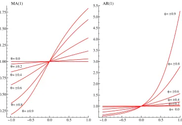
For AR(1) and MA(1) processes, the variance profile does not depend on the sign of the
pa-rameter ϕor θ and tends to an horizontal straight line when |ϕ|,|θ| →0. On the other hand, for
absolute values ofϕandθincreasing towards unity, the curves described byvp for an AR and a MA
process become different. Specifically, the plot of vp for MA(1) processes has an inflexion point in
p= 0, where the variance profile curve changes its concavity. This does not happen to the variance
profile graph of an AR(1) process which shows the same concavity for all the values of p∈[−1,1].
Indeed, the variance profile of an AR(1) process shows an inflexion point inp= 1 (see section 5.2).
Figure 1 evidences the difference between the variance profile of an autoregressive and a moving average process.
An interesting feature is thatp[lnvp−lnv0] for an AR(1) process with parameterϕis the same
asp[lnv−p−lnv0] for an MA(1) with parameterθ=ϕ.
5.2 Cycle models
A popular cyclical model is the circular model proposed by Harvey (1989) and West and Harrison (1989, 1997), see also Luati and Proietti (2010), which is an ARMA(2,1) process with complex conjugates AR roots and pseudo-cyclical behavior.
In the sequel we shall refer to the representation provided by Haywood and Tunnicliffe-Wilson (2000):
(1−2ρcosϖB+ρ2B2)yt=
√
G
2 (1 +B)κt+
√
H
2 (1−B)κ
∗
t (15)
whereϖ∈[0, π] is the cycle frequency, ρis a damping factor, taking values in [0,1), κt andκ∗t are
two uncorrelated white noise disturbances with variance σ2κ, and
G= sin2(ϖ 2
)
(1 +ρ)2+ cos2(ϖ 2
)
(1−ρ)2, H = sin2(ϖ 2
)
(1−ρ)2+ cos2(ϖ 2
)
Figure 1: Variance profiles for MA(1) and AR(1) processes with unit p.e.v.
−1.0 −0.5 0.0 0.5 1.0
0.25 0.50 0.75 1.00 1.25 1.50 1.75
MA(1)
θ= ±0.9 θ= ±0.8 θ= ±0.6 θ= ±0.4 θ= ±0.2 θ= 0.0
−1.0 −0.5 0.0 0.5 1.0
1.0 1.5 2.0 2.5 3.0 3.5 4.0 4.5 5.0 5.5 AR(1)
φ= ±0.9
φ= ±0.8
φ= ±0.6
φ= ±0.4
φ= 0.0 φ=±0.2
When ϖ= 0, yt is the AR(1) process (1−ρB)yt=ξt∼WN(0, σ2κ); whenϖ=π, (1 +ρB)yt=ξt. Finally, for ϖ=π/2, (1 +ρ2B2)y
t=
√
1 +ρ2ξ
t.
By integrating the Fourier transform of both sides of (15) we obtain
Var(yt) = σκ2 1−ρ2
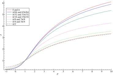
independently of the cycle frequency. Thus, the cycle models that differ only for the cycle frequency
are characterised by the same variance; however, the prediction error variance and the other vp
values,p̸= 1 will vary withϖ. Figure 2 illustrates this fact with reference to the case whenρ= 0.8
and σ2κ = 1−ρ2, so that Var(yt) = 1. The variance profiles have an inflection point atp = 1 and
forp→ ∞ converge to the maximum of the spectrum.
A seasonal component is modelled by summing trigonometric cycles defined at the fundamental
frequency and at the harmonic frequencies using the same scale parameterσ2
κ and the sameρ (e.g.
ρ→1 in nonstationary seasonal models, see Hannan, Terrell and Tuckwell, 1970, and Harvey, 1989).
In this case the individual cycles will be characterised by different predictability and interpolability; moreover, the maximum of the spectrum also varies.
To obtain cycle processes defined at different frequenciesϖ, but characterised by the same vp,
ρ and σ2 have to vary according to the expression
dρ
ρ =−
1 2(1−ρ
2)dσ2κ σ2
Figure 2: Variance profiles for cyclical models with ρ= 0.8 andσ2
κ = (1−ρ2)
0 and π
π/64 and 63π/64
π/32 and 31π/32
π/16 and 15π/16
π/8 and 7π/8
π/4 and 3π/4
π/2
−1 0 1 2 3 4 5 6 7 8 9 10
1 2 3 4 5 6
p vp
0 and π
π/64 and 63π/64
π/32 and 31π/32
π/16 and 15π/16
π/8 and 7π/8
π/4 and 3π/4
π/2
For instance, the process (1 + 0.912)yt= (1 +ρ2)0.5κt has the samevp as (1±0.8)yt=κt.
5.3 Variance profile for long memory processes
Let us consider the fractionally integrated noise (FN) process
xt= (1−B)−dξt, ξt∼WN(0, σ2), (16)
which is stationary for d < 1/2 and invertible for d > −1 (see Palma, 2007, Theorem 3.4 and
Remark 3.1). In this range,xt has Wold representation
xt=
∞
∑
j=0
Γ(j+d)
Γ(j+ 1)Γ(d)ξt−j,
autocovariance function
γ(h) =σ2 Γ(1−2d) Γ(1−d)Γ(d)
Γ(h+d) Γ(1 +h−d)
and spectrum f(ω) = (2π)−1σ2[2 sin(λ/2)]−2d. The variance profile is
vp =
[
Γ(1−2pd) Γ2(1−pd)
]1/p
σ2, dp <0.5
∞ dp≥0.5, d, p >0,
0 dp≥0.5, d, p <0,
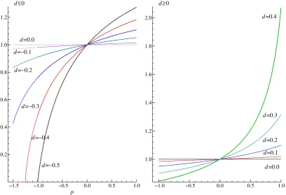
Figure 3: Variance profiles for fractional noise process with memory parameterd.
−1.5 −1.0 −0.5 0.0 0.5 1.0
0.2 0.4 0.6 0.8 1.0 1.2
d=−0.5 d=−0.4 d=−0.3 d=−0.2 d=−0.1 d=0.0
p d≤0
−1.0 −0.5 0.0 0.5 1.0
1.0 1.2 1.4 1.6 1.8
2.0 d=0.4
d=0.0 d=0.1 d=0.2 d=0.3 d≥0
When d ≤ −0.5 and p = −1 we obtain the result discussed in Walden (1994), which specialises
Grenander and Rosenblatt (1957, p. 84), i.e. the interpolation error variance of a non-invertible FN process is zero. For instance, letd=−1 in (16), so that xt=ξt−ξt−1.It follows immediately that
xt=∑∞j=1(xt+j−xt−j), so thatxtcan be perfectly interpolated from the infinite past and future.
In this case, analogous to the case of a deterministic process which occur when∫
log 2πf(ω) =−∞, the integral of [2πf(ω)]−1 does not exist.
Figure 3 displays the variance profiles for a FN process with varyingdvalues. Ford∈(−0.5,0.5)
and p ∈ (−1,1), vp exists and it is different from zero. It ought to be noticed that for negative
values of dthe variance profile is negatively convex, whereas ford >0 the convexity is positive.
When d > 0, the distinctive feature of the variance profile, as compared to a short memory
process with high persistence (e.g. an AR(1) withϕ= 0.9) is that vp→ ∞asp→(2−d), whereas
for the latter is converges to the finite maximum of the spectral density.
6
Estimation of the long memory parameter based on the variance
profile
A method of moments estimator of the long–memory parameterdof a fractionally integrated process
Table 1: Estimation of the long memory parameter: true value isd= 0.4
n= 500
Minimum distance estimator G-PH estimator
m= 3 m= 7 m= 11 m= 15 R= [n/16] R = [n/8] R= [n/4] R=n
Bias -0.0601 -0.0550 -0.0560 -0.0562 0.0071 0.0060 0.0057 0.0033
Std. err. 0.0481 0.0421 0.0463 0.0467 0.1373 0.0912 0.0624 0.0472
MSE 0.0059 0.0048 0.0053 0.0053 0.0189 0.0083 0.0040 0.0022
n= 1000
Minimum distance estimator G-PH estimator
m= 3 m= 7 m= 11 m= 15 R= [n/16] R = [n/8] R= [n/4] n
Bias -0.0431 -0.0408 -0.0418 -0.0417 0.0053 0.0038 0.0028 0.0020
Std. err. 0.0266 0.0270 0.0295 0.0319 0.0947 0.0671 0.0457 0.0339
MSE 0.0026 0.0024 0.0026 0.0027 0.0090 0.0045 0.0021 0.0012
between the sample and the theoretical variance profile in (17):
∫ b
a
k(p)(ˆvp(m)−vp)2dp.
In practice, in the persistent case (d > 0), we evaluate both (12) and (17) on a regular grid of p
values froma >−m/2 tob= 1. Asvpdepends also onσ2, we replace the latter by ˆσ2(m) = ˆv0(m); this yields the theoretical profile for an FN process characterised by the same p.e.v. estimated on
the time series. The weights k(p) may be uniform or inversely related to the asymptotic variance
Vp.
A Monte Carlo experiment using 5000 replications has been performed to assess the properties
of the proposed estimator (k(p) = 1), when the true memory parameter isd= 0.4. For comparison
of the bias, standard error and the mean square error we also report the same quantities for the widely applied Geweke and Porter-Hudak (1983) estimator
˜ d=
∑R
j=1[lnI(ωj)(wj−w¯)]
∑R
j=1(wj−w¯)2
,
based on the least squares regression of lnI(ωj) on a constant and wj = −2 ln(2 sin(ωj/2)), j = 1, . . . , R, where ¯w=R−1∑R
j=1wj.
The simulation evidence, presented in table 1, shows that forn= 500 andn= 1000 our proposed
estimator performs as efficiently as the GPH using n/8 periodogram ordinates. The value of m
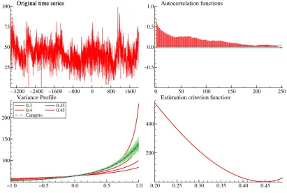
Figure 4: Mount Campito tree rings data: series (top left panel); sample autocorrelation function
(top right), estimate of the variance profile using m = 23 (bottom left) and estimation criterion
(ˆvp(m)−vp)′(ˆvp(m)−vp), where the variance profile is evaluated in an equally spaced grid of values in the range (-6, 1).
−3200 −2400 −1600 −800 0 800 1600
25 50 75
100 Original time seriesOriginal time series
0 50 100 150 200 250
−0.5 0.0 0.5
1.0 Autocorrelation functions
0.3 0.4 Campito
0.35 0.45
−1.0 −0.5 0.0 0.5 1.0
100 150 200
Variance Profile 0.3
0.4 Campito
0.35 0.45
0.20 0.25 0.30 0.35 0.40 0.45
200 400
Estimation criterion function
7
Empirical Illustrations
7.1 Mount Campito tree rings data
The Mount Campito data is a popular time series consisting of 5405 annual values of bristlecone pine tree ring widths, spanning the period from the year 3426 BC to 1969 AD. The series is plotted in the upper left panel of figure 4; the sample autocorrelations are persistently positive and decay very slowly (see upper right panel).
The estimated variance profile is that of a long memory process with high d. It is displayed
in the bottom left panel along with the 95% interval estimates, computed as ˆvp(m)±1.96
√
ˆ
Vp/n
using m= 23. The long memory parameter is estimated equal to 0.448, a value in accordance with
the literature see e.g. Baillie (1996, page 45). The estimation criterion function is plotted in the last panel.
7.2 Power transformation of absolute returns
Let rt denote an asset return. Ding, Granger and Engle (1993) addressed the issue of determining
property of the transformed series
xt(λ) =|rt|λ
is strongest. Focusing on the Standard & Poor stock market daily closing price index over the
period 3/1/1928-30/8/1991, they argued that the long memory property is strongest when λ= 1.
The analysis of two time series of returns according to the variance profile provides a broad confirmation of these findings. We focus on the daily returns computed on the Nasdaq and Standard & Poor stock market daily closing price index, available for the sample period 3/1/1989 - 7/3/2011
(n= 10110). As we may record zero returns we adopt the shifted-mean power transformation (see
Atkinson, 1985)
xt(λ) = (|rt|+c)λ,
where c= 0.001 (the choice of c turns out to be unimportant).
An issue arises as to whether normalised Box-Cox transform or the standardised one should
be considered. The former is obtained by dividing xt(λ) by n
√
J, where J = ∏
t
∂xt(λ)
∂xt
is the
Jacobian of the transformation, (Atkinson, 1985). We prefer the second solution, as we would like to determine the transformation for which the series has the smallest normalised variance profile.
In other words, we will constraint v1 = 1 for all theλvalues.
Setting m = 17 we estimate the variance profile for the standardised transformed series for
values of λin the interval (−0.5,2.3). The results for the SP500 series are presented in figure 6.
The variance profile of the standardisedxt(λ) can be used to determine the value of the
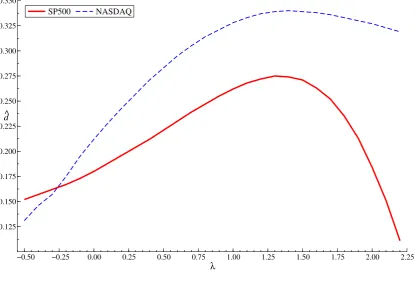
trans-formation parameter for which the long memory property is strongest. Figure 5 plots the value of
the value of d, estimated according to section 4, against λ. It turns out that for both series the
maximumdis achieved forλaround 1.25. However, the variance profile does not differ significantly
for that associated to λ= 1, which does not contradict Ding, Granger and Engle (1993).
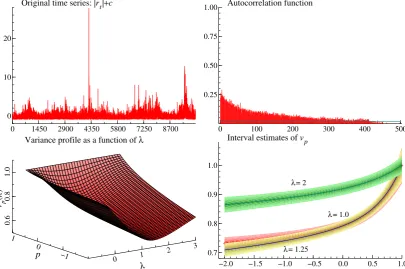
This fact is illustrated by figure 6, which refers to the SP500 series, displayed in the top right
panel. The plot also shows that the normalised variance profile is a minimum forλin the vicinity
of 1.25. The last display shows the interval estimates of vp forλ = 1,1.25 and 2. It can be seen
that the variance profile for the absolute returns does not differ from that for λ = 1.25, whereas
the squared returns (λ= 2) differ significantly. The implication is that the squared returns are less
predictable and interpolable than the absolute returns. Another conclusion is that the volatility of Nasdaq returns is more predictable than SP500’s.
7.3 The Great moderation
Figure 5: Nasdaq and SP500 daily absolute returns: estimates of the long memory parameter d
based on the variance profile as a function of the transformation parameterλ.
SP500 NASDAQ
−0.50 −0.25 0.00 0.25 0.50 0.75 1.00 1.25 1.50 1.75 2.00 2.25
0.125 0.150 0.175 0.200 0.225 0.250 0.275 0.300 0.325 0.350
λ ^
d
Figure 6: Standard and Poor 500 daily absolute returns (standardised): variance profile as a function of the Box-Cox transformation parameter: series (top left panel); sample autocorrelation
function (top right), estimate of the variance profile using m= 17 (bottom left) and comparison of
the interval estimates for λ= 1,1.25 and λ= 2.
0 1450 2900 4350 5800 7250 8700
0 10 20
Original time series: |rt|+c
0 100 200 300 400 500
0.25 0.50 0.75
1.00 Autocorrelation function
λ
Variance profile as a function of λ
p vp
(
λ
)
0 1
2 3
−1 0 1
0.6
0.8
1.0
−2.0 −1.5 −1.0 −0.5 0.0 0.5 1.0
0.7 0.8 0.9 1.0
Interval estimates of vp
λ= 2
λ= 1.0
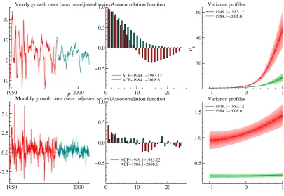
The variance profile can provide further insight on this issue. We focus on the U.S. monthly index of industrial production, made available by the Federal Reserve Board, both in seasonally adjusted and unadjusted form. We set off analysing the series of yearly growth rates for the period 1949.1-2008.6, which is split into two subseries, the first covering the period predating the GM (1949.1-1983.12) and the second covering the GM period (1984.1-2008.6). The series are plotted in figure 7; the volatility reduction is indeed visible and the patterns of the autocorrelations are also different - the behaviour is less cyclical in the GM period.
The estimated variance profile (using m = 7) for the two subperiods reveals that both the
variance and the prediction error variance are significantly reduced in the GM period. Forp→ −1
ˆ
vp gets very close to zero for both subseries. This is a likely consequence of the fact that seasonality
in the original series is very stable, so that the yearly growth rates are likely to be non-invertible
at the seasonal frequencies as a result of the application of the filter (1−B12).
When we come to the monthly growth rates (computed on the seasonally adjusted series), see the bottom panel of figure 7, we also find a significant change in the variance profile, which flattens downs to an almost horizontal pattern.
It should be noticed, however, that even though the GM is associated to a significant drop in the prediction error variance (v0), the relative predictability, 1−v0/v1, decreased, as well as the
interpolability, as measured by the index of linear determinism 1−v−1/v1.
8
Conclusions
The paper has introduced the variance profile and has proposed an estimator based on the smoothed periodogram, which generalises the Hannan and Nicholls (1977) estimator of the prediction error variance. The variance profile estimator was shown to be asymptotically normal and consistent.
Figure 7: U.S. Index of industrial production, yearly (seasonally unadjsted) and monthly growth rates (seas. adj.) for the two subperiods 1949.1-1983.12 (pre) and 1984.1-2008.6 (Great
Mod-eration). Comparison of autocorrelation function, variance profile and relative index 1−vp/v1.
1950 2000
−10 0 10 20
Yearly growth rates (seas. unadjusted series)
ACF−1949.1−1983.12 ACF−1984.1−2008.6
0 10 20
−0.5 0.0 0.5
1.0 Autocorrelation function
ACF−1949.1−1983.12 ACF−1984.1−2008.6
1949.1−1983.12 1984.1−2008.6
−1 0 1
20 40 60
Variance profiles
p
vp
1949.1−1983.12 1984.1−2008.6
1950 2000
−2.5 0.0 2.5 5.0
Monthly growth rates (seas. adjusted series)
ACF−1949.1−1983.12 ACF−1984.1−2008.6
0 10 20
−0.5 0.0 0.5
1.0 Autocorrelation function
ACF−1949.1−1983.12 ACF−1984.1−2008.6
1949.1−1983.12 1984.1−2008.6
−1 0 1
0.5 1.0 1.5
Appendix
We provide the proof of the consistency and asymptotic normality of the estimator
ˆ
vp(m) =m
1 M
M−1
∑ j=0 ( 1 m m ∑ k=1
2πI(ωjm+k)
)p
Γ(m) Γ(m+p)
1
p
.
We start from the case when p̸= 0; the case whenp→0 will be considered afterwards.
Form odd, the quantity m1 ∑m
k=12πI(ωjm+k) can be interpreted as a Daniell type estimator for 2πf(ωjm+m+1
2 ). Hence, assumingM and m large enough for asymptotics and
m
M small enough for
f(ω) to be constant over frequency intervals of length 2Mπm, for fixedm, and for 1≤k≤m,
m
∑
k=1
I(ωjm+k)
1
2f(ωjm+m+1 2
) ∼χ
2 2m
(see Koopmans, 1974, pp. 269-270) and therefore
m
∑
k=1
2πI(ωjm+k) = 2πf(ωjm+m+1 2 )Xj
where the Xj are independent and identically distributed random variablesXj ∼ 12χ22m or
equiva-lently, Xj ∼G(m,1),a basic Gamma random variable with shape parameter equal to m. Thus,
( m ∑
k=1
2πI(ωjm+k)
)p
=(2πf(ωjm+m+1 2 )
)p
Xjp. (18)
By direct integration,
E(Xjp)= Γ(m+p)
Γ(m) (19)
and by the usual formula for the variance of a random variable one gets,
Var(Xjp) = Γ(m+ 2p)
Γ(m) −
Γ2(m+p)
Γ2(m) , (20)
which exist for p >−m2. Hence, the random variable Zj defined as
Zj =
Xjp−Γ(Γ(mm+)p)
√
Γ(m+2p) Γ(m) −
Γ2(m+p) Γ2(m)
, (21)
has zero mean and unit variance.
Under the assumption of a uniformly bounded power of the spectral density function and by approximating the integral with its Riemannian sum,
1 2π
∫ π
−π
(2πf(ω))2pdω= lim M→∞
1 M
M−1
∑
j=0
(
2πf(ωjm+m+1 2 )
)2p
the quantity
QM = 1 M
M−1
∑
j=0
(
2πf(ωjm+m+1 2 )
)2p
exists and has a limit, limM→∞QM =v22pp. Let now
bj =
(
2πf(ωjm+m+1 2 )
)p
√
M QM
, (23)
which satisfies
M−1
∑
j=0
b2j = 1. (24)
Moreover, since thep-th power of the spectral density function is uniformly bounded and sinceQM
converges to a positive term, we have that
max
0≤j≤M−1|bj| →0.
Hence the assumptions for the central limit theorem for linear combinations of sequences of random variables (Gleser, 1965, Theorem 3.1, which relates to Eicker, 1963, and Gnedenko and Kolmogorov, 1954) are satisfied and
M−1
∑
j=0
bjZj →dN(0,1).
It follows by (21) and (24) that
M−1
∑
j=0
bjXjp→dN
M−1
∑
j=0
bjΓ(m+p)
Γ(m) ,
(
Γ(m+ 2p)
Γ(m) −
Γ2(m+p) Γ2(m)
)
and, as a function of our estimator, using (23),
{vˆp(m)}p= 1 M
√
M QM M−1
∑
j=0
bjXjp
Γ(m)
Γ(m+p) →dN
1 M
M−1
∑
j=0
(
2πf(ωjm+m+1 2 )
)p
,ΩM
(25)
where
ΩM =
1 MQM
(
Γ(m+ 2p)
Γ(m) −
Γ2(m+p) Γ2(m)
) (
Γ(m) Γ(m+p)
)2
.
By taking the limits
√
M({ˆvp(m)}p−vpp)→dN
(
0, v22pp
(
Γ(m+ 2p)Γ(m)
Γ2(m+p) −1
))
(26)
and applying the delta method we finally get the asymptotic distribution
√
n(ˆvp(m)−vp)→dN
(
0,2m
(
vp p
)2(
v2p vp
)2p(
Γ(m+ 2p)Γ(m)
Γ2(m+p) −1
))
We now prove the consistency of ˆvp(m) forvp, that is a consequence of three facts: the Chebychev weak law of large numbers, applied to the sequence of random variables Yj =√M QMbjXjΓ(Γ(mm+)p)
in ˆvp(m)p, see equation (25); the convergence of the Riemannian sum to the integral, see equation
(22); the Slutsky theorem for the probability limit, which allows us to state that since ˆvp(m)p,
is consistent for vpp then ˆvp(m) is a consistent estimator for vp, given that the power function is continuous.
Let us now considerp→0. In this case, the estimator (12) equals the prediction error variance
estimator (11), see equation (13); moreover, in this context, the case p → 0 correspond to the
case when the logarithm of Xj is taken, rather then its power, i.e. when p →0, Xjp is to be read
as logXj. Hence, E (exp{tlogXj}), given in equation (19), is the moment generating function of
logXj and gives E (logXj) = ψ(m) and Var (logXj) =ψ′(m). Therefore, when p → 0, equation
(18) becomes (some parentheses are omitted for sake of notation)
log m
∑
k=1
2πI(ωjm+k) = log 2πf(ωjm+m+1
2 ) + logXj
with
E log
( m ∑
k=1
2πI(ωjm+k)
)
= log 2πf(ωjm+m+1
2 ) +ψ(m)
and
Var log
( m ∑
k=1
2πI(ωjm+k)
)
=ψ′(m),
respectively. What follows is that in the limit case, the bias correction via a multiplication (by the inverse expected value, see equation (25)), becomes a subtraction and the subtracted quantity does
not modify the asymptotic variance of the estimator of the quantity (E(Xjp))−2. Specifically, when
p→0 ˆvp(m)p takes the following form
log ˆσ2(m) = 1 M
M−1
∑
j=0
(
log 2πf(ωjm+m+1
2 ) + logXj−ψ(m)
)
,
i.e. the sample means ofM random variables each one having expected value log 2πf(ωjm+m+1
2 ) and
varianceψ′(m). Since the variables are uniformly integrable (as implied by assuming that logf(ω) is
uniformly bounded for allω) the central limit theorem applies and, since M1 ∑M−1
j=0 logf(ωjm+m+1 2 ),
√
M(log ˆσ2(m)−logσ2)→dN(0, ψ′(m))
and replacing M = (n−1)/(2m) and by the delta method,
√
n(ˆσ2(m)−σ2)→dN(0,2mσ4ψ′(m)).
The case when m = 1, is a particular case of (12). However, one could note that when m = 1
the estimator (12) becomes
ˆ vp =
1 N
N
∑
j=1
[2πI(ωj)]p[Γ(p+ 1)]−1
1
and the random variables involved in its asymptotic distributions can be written as monotonic transforms ofχ22 random variables, asYj = [2πI(ωj)]p =[
πf(ωj)χ22]p
.It follows that forp̸= 0, by applying the density transform method one gets
fY j(y) =
1
|p|
[2πf(ωj)]p
(
y [2πf(ωj)]p
)1
p−1
exp
{
−
(
y [2πf(ωj)]p
)1
p
}
.
When pis positive and finite, then fY j(y) is the density of a Weibull distribution with parameters
(α, β) whereα = 1p, β = [2πf(ωj)]p; on the other hand, when p is negative, then Yj is distributed
like a Frech´et random variables with the same parameters. Note that when p → 0 we find the
Gumbel distribution, i.e. the distribution of the logarithm of an exponential random variable,
that coincides with Davis and Jones (1968) distribution of the log-periodogram. For p >−12, the
expected value and the variance of the Yj are given by
E(Yj) = [2πf(ωj)]pΓ(p+ 1)
Var(Yj) = [2πf(ωj)]2p
[
Γ(2p+ 1)−Γ2(p+ 1)]
from which follows that the random variablesZj =YjΓ(p+ 1)−1 have mean and variance given by
E (Zj) = [2πf(ωj)]p
Var(Zj) = [2πf(ωj)]2p
[
Γ(2p+ 1)Γ−2(p+ 1)−1]
.
and since they are uniformly bounded the Lindeberg-Feller central limit theorem applies and we
get (26) and (27) with m= 1.
Note that forp >0 we find the result of Corollary 1 in Taniguchi (1980), which requires positivity of the exponent for existence of the inverse Laplace transform upon which his estimator is based.
Finally, it is straightforward to verify that when p → 0 and m = 1 we find the asymptotic
References
[1] Atkinson, A. C. (1985), Plots, Transformations and Regression: An Introduction to Graphical
Methods of Diagnostic Regression Analysis, Oxford University Press, Oxford, UK.
[2] Baillie, R.T. (1996), Long memory processes and fractional integration in econometrics,Journal
of Econometrics, 73, 5, 1–59.
[3] Battaglia, F., Bhansali, R. (1987), Estimation of the Interpolation Error Variance and an Index
of Linear Determinism,Biometrika, 74, 4, 771–779.
[4] Bhansali, R. (1993), Estimation of the Prediction Error Variance and an R2 Measure by
Au-toregressive Model Fitting,Journal of Time Series Analysis, 14, 2, 125–146.
[5] Box, G.E.P., and Cox, D.R. (1964), An analysis of transformations (with discussion), Journal
of the Royal Statistical Society, B, 26, 211–246.
[6] Chatfield, C.S. (1972), Inverse Autocorrelations,Journal of the Royal Statistical Society, Series
A, 142, 3, 363–377.
[7] Choudhuri, N., Ghosal, S., Roy, A. (2004), Bayesian Estimation of the Spectral Density of a
Time Series,Journal of the American Statistical Association, 99, 468, 1050–1059.
[8] Cleveland, W.S. (1972), The Inverse Autocorrelations of a Time Series and Their Applications,
Technometrics, 14, 2, 277–293.
[9] Davis, H.T. and Jones, R.H. (1968), Estimation of the Innovation Variance of a Stationary
Time Series,Journal of the American Statistical Association, 63, 321, 141–149.
[10] Diebold, F.X. and Kilian, L. (2001), Measuring Predictability: Theory and Macroeconomic
Applications,Journal of Applied Econometrics, 16, 657–669.
[11] Ding, Z., Granger, C.W.J. and Engle, R.F. (1993), A long memory property of stock market
returns and a new model,Journal of Empirical Finance, 1, 1, 83–106.
[12] Eicker F. (1963), Central Limit Theorems for Families of Sequences of Random Variables,The
Annals of Mathematical Statistics, 34, 2, 439–446.
[13] Geweke, J. and Porter-Hudak, S. (1983), The Estimation and Application of Long-Memory
Time Series Models,Journal of Time Series Analysis, 4, 221–238.
[14] Gleser L.J. (1965), On the Asymptotic Theory of Fixed-Size Sequential Confidence Bounds
for Linear Regression Parameters,The Annals of Mathematical Statistics, 36, 2, 463–467.
[15] Gnedenko, B.V. and Kolmogorov, A.N. (1954),Limit Distributions for Sums of Random
Vari-ables, Addison-Wesley Publishing Company.
[16] Janacek, G. (1975), Estimation of the Minimum Mean Square Error of Prediction,Biometrika,
[17] Johnson N.L. and Kotz, S. (1972), Power Transformations of Gamma Variables, Biometrika, 59, 1, 226–229.
[18] Hannan, E.J. and Nicholls, D.F. (1977), The Estimation of the Prediction Error Variance,
Journal of the American Statistical Association, 72, 360, 834–840.
[19] Hannan, E.J., Terrell, R.D., and Tuckwell, N.E. (1970), The seasonal adjustment of economic
time series,International Economic Review, 11, 24–52.
[20] Harvey, A.C. (1989), Forecasting, Structural Time Series Models and the Kalman Filter,
Cambridge University Press.
[21] Haywood, J. and Tunnicliffe-Wilson, G. (2000), An Improved State Space Representation for
Cyclical Time Series,Biometrika, 87, 3, 724–726.
[22] Kensahara, Y., Pourahmadi, M. and Inoue, A. (2009), Duals of Random Vectors and Processes
with Applications to Prediction Problems with Missing Values,Statistics and Probability Letters,
79, 1637–1646.
[23] Kohli, P. and Pourahmadi, M. (2011), Nonparametric estimation of the innovation variance and judging the fit of ARMA models, forthcoming in Bell, W.R., Holan, S.H. and McElroy T.
(eds)Economic Time Series: Modeling and Seasonality, Chapman and Hall/CRC.
[24] Kolmogorov, A.N. (1941), Interpolation and Extrapolation of Stationary Random Sequences
(in Russian),Izv. Akad. Nauk SSSR Sere Mat., 5, 3–14.
[25] Kolmogorov, A.N. (1992), Interpolation and Extrapolation of Stationary Random Sequences, inSelected works of A.N. Kolmogorov, Volume II, Probability and Mathematical Statistics, 272– 280.
[26] Koopmans, L.H. (1974),The Spectral Analysis of Time Series, Academic Press.
[27] Luati, A. and Proietti, T. (2010), Hyper-spherical and Elliptical Stochastic Cycles, Journal of
Time Series Analysis, 31, 169–181.
[28] Masani, P. (1960), The prediction theory of multivariate stochastic processes, III Unbounded
spectral densities,Acta Mathematica, 104, 1-2, 141–162.
[29] McConnell, M.M. and Perez-Quiros, G. (2000), Output Fluctuations in the United States:
What Has Changed since the Early 1980’s?,American Economic Review, 90, 1464–1476.
[30] Nelson, C.R. (1976), The Interpretation of R2 in Autoregressive-Moving Average Time Series
Models,The American Statistician, 30, 175–180.
[31] Pukkila, T. and Nyquist, H. (1985), On frequency domain estimation of the innovation variance
of a stationary univariate time series.Biometrika, 72, 317323.
[32] Salehi, H. (1979), Algorithms for Linear Interpolator and Interpolation Error for Minimal
[33] Szeg¨o, G. (1920), Beitrage zur Theorie der Toeplitzen Formen (Ersten Mit- teilung), Mathe-matische Zeitschrift, 6, 167-202.
[34] Szeg¨o, G., Askey, R. (1982),Gabor Szeg¨o: Collected Papers, Vol. 1: 1915-1927, Birkauser.
[35] Stock, J.H., and Watson, M.W. (2002), Has the Business Cycle Changed and Why? NBER
Macroeconomics Annual, 17, 159–230, National Bureau of Economic Research.
[36] Taniguchi, M. (1980), On Estimation of the Integrals of Certain Functions of Spectral Density,
Journal of Applied Probability, 17, 1, 73–83.
[37] Tong, H. (1979), Final Prediction Error and Final Interpolation Error: A Paradox?, IEEE
Transactions on Information Theory, It-25, 6, 758-759.
[38] Walden, A. T. (1995), Multitaper estimation of innovation variance of a stationary time series,
IEEE Transactions on Signal Processing, 43, 181-187.
[39] Walden, A. T. (2000), A unified view of multitaper multivariate spectral estimation.
Biometrika, 87, 767-788.
[40] West, M.and Harrison, J. (1989),Bayesian Forecasting and Dynamic Models, 1st edition, New
York, Springer-Verlag.
[41] West, M.and Harrison, J. (1997),Bayesian Forecasting and Dynamic Models, 2nd edition, New
York, Springer-Verlag.
[42] Wiener, N. (1949),Extrapolation, Interpolation and Smoothing of Stationary Time Series, The