Laminar Turbulent Boundary Layer Transition Imaging Using IR Thermography

Laminar-Turbulent Boundary Layer Transition Imaging

Using IR Thermography

Brian K. Crawford, Glen T. Duncan Jr., David E. West, William S. Saric Department of Aerospace Engineering, Texas A&M University, College Station, USA

Email: [email protected]

Received May 1, 2013; revised June 1, 2013; accepted June 8, 2013

Copyright © 2013 Brian K. Crawford et al. This is an open access article distributed under the Creative Commons Attribution Li-cense, which permits unrestricted use, distribution, and reproduction in any medium, provided the original work is properly cited.

ABSTRACT

Experimental techniques for imaging laminar-turbulent transition of boundary layers using IR thermography are pre- sented for both flight and wind tunnel test environments. A brief overview of other transition detection techniques is discussed as motivation. A direct comparison is made between IR thermography and naphthalene flow visualization. A technique for obtaining quantitative transition location is presented.

Keywords: IR Thermography; Laminar; Turbulent; Transition; Flight Test; Wind Tunnel; Fluid Flow

1. Introduction

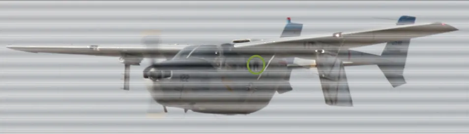
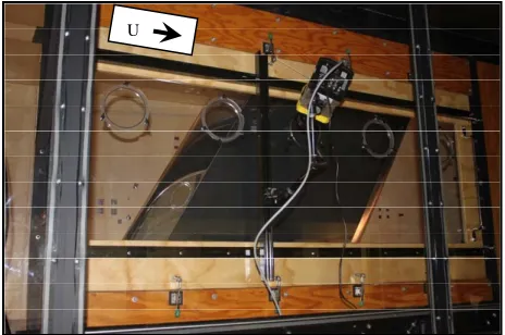
Over the past several years, laminar flow research has been ongoing at the Texas A&M Flight Research Labo- ratory (FRL) using both the Swept Wing In Flight Test- ing (SWIFT) and Swept Wing In Flight Testing Excres- cence Research (SWIFTER) models. Both models were designed to be mounted to the hardpoint of a Cessna O- 2A Skymaster aircraft, and use IR thermography as the primary measurement technique for laminar-turbulent transition imaging. Figures 1 and 2 show SWIFTER mounted under the port wing. SWIFT has the same outer dimensions and is mounted on the same pylon when it is flown.

IR thermography exploits the fact that when there ex- ists a temperature differential between the surface of an airfoil and the ambient fluid, the turbulent region will

tend to equalize to the ambient temperature faster due to its higher shear stress. This difference in temperature can be imaged using IR thermography [1-3]. The two models differ in how they achieve this differential. SWIFT is cooled by cold soaking at 3200 m MSL until it equalizes to ambient temperature. The aircraft then descends rap- idly through warmer air. SWIFTER, on the other hand, has an internal heating sheet that is used to warm the sur- face above ambient. As such, SWIFTER does not require a high-altitude cold soak. Additionally, since SWIFTER does not rely on an externally applied temperature dif- ferential, it is also capable of utilizing IR thermography when installed in a wind tunnel which operates under adiabatic conditions. An example of SWIFTER in the Klebanoff-Saric Wind Tunnel (KSWT) is shown in Fig- ure 3.

Figure 2. SWIFTER as viewed from the pilot.

U

Figure 3. SWIFTER Mounted in the KSWT along with the

2. Motivation

a significant portion of a transport air-

ent transition de- te

su

local pressure flu

sualization involves apply- in

pl

t can be used to image shear stress ov

ary, most existing techniques for boundary la

3. Theory

fferences in shear stress, laminar and turbu-

exploited experimentally by utilizing a he

SC8100 IR Camera.

Laminarization of

craft wing would result in an estimated overall drag sav- ings of 15% [4]. This would result in considerable fuel savings for any such aircraft; however, in order to make reliable laminar flow a reality, it must be studied and quantified in a laboratory environment.

Several techniques for laminar-turbul

ction have been developed and implemented over the last several decades. Some of the more common tech- niques include hot-film anemometry, surface-mounted microphones, sublimation based flow visualization, shear sensitive paint, and oil-film interferometry. A review of options for laminar-turbulent transition is given in [5].

Hot-film anemometry provides local shear stress mea- rements. These local shear stress measurements can be used to detect whether flow is laminar or turbulent over the sensor as shown in [6]. However, to image an entire transition front, many sensors are needed. This becomes unfeasible when mm accuracy is desired.

Surface-mounted microphones measure

ctuations. Turbulent flow can be detected by a large rise in the broadband oscillations in pressure. However, much like hot-films, the number of microphones required to image an entire transition front to sub centimeter ac- curacy becomes infeasible.

Sublimation based flow vi

g a coating of naphthalene or similar chemical to the surface under test and allowing the chemical to sublimate off during the experiment. The turbulent region subli- mates much faster than the laminar region, and as such, the resulting pattern of remaining naphthalene indicates what part of the flow is laminar. This technique can pro- vide excellent images, but requires complete sublimation and re-application for every test point. Reference [7] pro- vides examples of this technique in a flight environment.

For oil film interferometry, multiple drops of oil are aced on the model. When the model is brought up to speed, the oil shears proportionally with the local shear stress. The shearing of the oil is then measured optically, and the variation in shear can be used to detect regions of laminar vs. turbulent flow. The down side is that this technique relies on conditions being constant for the du- ration of the test, and must be re-applied for every test. Additionally, oil residue can pose an issue in a clean tunnel environment. Further details on this technique can be found in [8].

Shear sensitive pain

er the entire surface. However, shear sensitive paints that are capable of measuring relatively low shear stress are very fragile, and must be re-applied somewhat fre- quently. As shear sensitive paint technology improves, this may become a practical technique for imaging lami- nar-turbulent transition in many environments. Reference [9] provides more information on the use of shear sensi- tive paint.

In summ

yer transition have limited fidelity, as is the case with hot-films and surface microphones or require extended time on very stable conditions, naphthalene flow visuali- zation and oil film interferometry. In order to detect tran- sition fronts rapidly with high fidelity, a technique such as infrared thermography is required.

Because of di

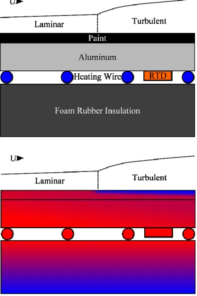
lent boundary layers have markedly different convection coefficients. As such, a heated surface will cool much faster under the influence of a turbulent boundary layer than under a laminar boundary layer; visa-versa for a cooled surface.

This can be

sonably uniform rate from below by the substrate, but is under the influence of a very discontinuous convection rate from above, a strong temperature gradient is devel- oped at the point of transition. This gradient can then be imaged via the use of an IR camera. A notional diagram of this process is shown in Figure 4.

4. Experimental Setup

concerned, the experiment

4.1. Cooled Model

from milled aluminum. The model As far as IR thermography is

requires three main components; an IR camera, a heated or cooled model, and a suitable thin, insulating coating on the model.

SWIFT is constructed

itself has no specific provisions for cooling. Instead, the model is cold soaked at 3200 m MSL until the IR image shows that it has equalized to the local atmospheric tem- perature. This typically takes around 20 minutes. Once the model is cool, the aircraft then rapidly descends through the warmer air at lower altitudes. At a 300 - 600 m/min descent rate, the standard lapse rate of the atmos- phere is sufficient to induce the necessary temperature differential. However, the necessary descent rate will vary based on model construction and local atmospheric

conditions. Reference [10] contains addition information about the SWIFT model.

4.2. Heated Model

Figure 4. Construction of heated model (not to scale) (top) Temperature distribution near transition (bottom).

nstructed from milled aluminum. SWIFTER is also co

Due to structural considerations, the model has two dis- tinct regions of wall thicknesses; a forward and aft region. In the forward region, the skin is between 12.7 mm and 25.4 mm. In the aft region, the skin is 3.2 mm thick. Thus, the heating sheet for the model is split into two regions, one forward and one aft, which run on separate control loops in order to keep the two regions matched in tempe- rature. The forward and aft heating sheets have a maxi- mum power of 200 W (792 W/m2) and 300 W (350 W/m2), respectively.

The heating sheet itself was constructed using pre- sheathed heating wire. This particular wire is typically used to warm tile floors in houses from below. The heat- ing wire is bonded onto the inside of the test surface of the model via RTV silicone, as shown in Figure 5. In the forward region, the wire is bonded in at 12.7 mm spacing, while the aft region is spaced at 25.4 mm. It is covered by a layer of 12.7 mm polyurethane foam to help direct as much of the heat as possible through the test surface.

The temperature controller is connected to a pair of surface mounted resistance temperature detectors (RTDs) placed on the inside surface of the test section inside each of the two heating sheets. There is also a reference RTD placed on the inside of the unheated side of the model. During a test, the controller is generally set to drive the test side RTDs to 5˚C higher than the reference RTD. Since these measurements are on the inside of the model, they do not match the external surface tempera- tures exactly. However, they do maintain a surface tem- perature that is consistent between the two regions, and nominally a constant offset from the atmospheric tem- perature. For this imaging technique, the exact tempera-

Figure 5. Heating wire (blue) bonded into SWIFTER usin RTV (red) with the insulation (black) pulled back.

ture offset is not important, as long as the model is a few degrees warmer than ambient. Additional details about the SWIFTER model can be found in [11].

4.3. IR Camera

Early experiments with SWIFT utilized a FLIR SC3000 IR camera. The SC3000 has a 320 × 240 pixel sensor with a maximum frame rate of 60 Hz. It operates in the 8 - 9 micron wavelength band.

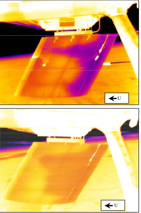
Later experiments with SWIFT, and all experiments with SWIFTER utilize a FLIR SC8100 IR camera. The SC8100 has a 1024 × 1024 pixel sensor capable of sam- pling at 132 Hz. It has a temperature resolution of better than 25 mK, and operates in the 3 - 5 micron wavelength band. For these experiments, the frame rate is typically set to 20 Hz in order to reduce data overhead. Addition- ally, the system does not respond rapidly enough to war- rant a higher frame rate. Figure 6 shows a comparison between the two cameras.

In the flight environment, the camera is mounted fac- ing outwards through an opening in the rear port window, as seen just above the port wing strut in Figure 1. In the

U U

wind tunnel, the camera is mounted facing through an opening in the test section viewing window, as shown in

Figure 3. In both cases, an opening in the window is utilized rather than an IR transparent window. This is due to the substantial cost of an IR transparent window large enough to fit the camera lens.

4.4. Paint Selection

Figure 6. SWIFT using the SC8100 w/17 mm lens (top) vs. the SC3000 w/17 mm lens (bottom).

ly, the model must be coated with

phy has been used in three principle con-

iscussed in Sec- As mentioned previous

a thin insulating layer in order to hold a strong tempera- ture gradient. Additionally, the coating must have as low of a reflectivity in the IR band as possible. This is par- ticularly important in flight where the exhaust flare from the front engine and the warm earth reflect brightly in the image otherwise. In order to meet these parameters, Sherwin Williams F93 mil-spec aircraft paint in luster- less black is currently used on SWIFTER.

SWIFT has a flat black powder coated surface applied over aluminum. This coating holds a gradient well, but is fairly reflective in the IR band.

Initially SWIFTER had a flat black powder coat as well. However, that particular coating was not thick en- ough to hold a strong temperature gradient at the surface; as such, the images were completely washed out. Addi- tionally, the powder coat was very reflective in the IR band. The new aircraft paint is very flat in the IR band. The new paint was applied over the existing powder coat to a total thickness on the order of 300 microns. The thicker paint results in a much crisper image.

5. Results

IR thermogra

figurations at the TAMU FRLand KSWT. The first con- figuration used SWIFT as a cooled flight model. This was followed recently by SWIFTER as a heated flight model as well as a heated wind tunnel model.

5.1. Cooled Flight Model (SWIFT)

Cooling the model via cold soaking, as d

tion 4.1, results in images such as shown in Figures 6

Figure 7. SWIFT using the SC8100 w/50 mm lens.

the m ular

owder coat.

oak is that it does not require any addition eq

sadvantage. only neces-

d Tunnel Model (SWIFTER)

Since SWIFTER can be mounted in the wind tunnel, it odel. This is due to the reflectivity of the partic p

The primary advantage to cooling a model via high- altitude cold s

uipment or coatings on the model, other than a suitable paint job. However, every set of tests requires a 20 min- ute cold soak. Given a typical descent rate during a test, a high speed descent from 3200 m to 900 m allows for around 5 - 10 test points before the model must be cold soaked again depending on atmospheric conditions. For a typical sortie with an O-2A Skymaster, two dives are practical, resulting in 10 - 20 test points per flight.

5.2. Heated Flight Model (SWIFTER)

Actively heated models do not share this di For a heated model, a high speed descent is

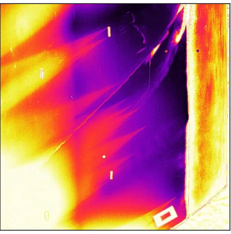
sary in order to hit high speed test points. Additionally, no appreciable recycle time is required between dives. As such, 6 dives of 5 - 10 test points are typical. This results in 30 - 60 test points per flight. The only real disadvan- tage is that the extra complexity of a heating sheet must be integrated into the model. However, compared to the cost of flight time saved by increased testing efficiency, this additional start-up cost is quickly recovered. An example image is shown in Figure 8. Note that when the model is heated, the image coloration is inverted com- pared to the cooled case. In Figure 8, the vertical seam between the forward and aft regions is visible due to transient effects.

5.3. Heated Win

U

U

Figure 8. SWIFTER using the SC8100 w/ 50mm lens Full image (top), and zoomed in on mid-span (bottom).

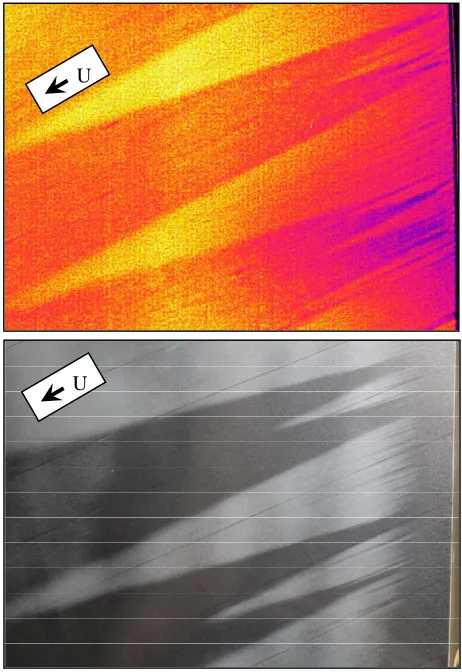
lization. provides an opportunity to compare IR thermography to

he more ubiquitous naphthalene flow visua t

U

U

Figure 9. SWIFTER transition fronts in the wind tunnel at a repeated condition using IR thermography (top), and naphthalene flow visualization (bottom).

second, while aphthalene would require a complete re-application. Be-

phy, e data. age as

pix- el

its quick turnaround time. When the transition front changes, the image responds in under a

n

cause of this fact, an IR thermography test can easily capture over 200 test points in an hour, while a typical day of naphthalene runs involves only 3 test points.

5.4. Post-Processing of Transition Images

Once images have been captured via IR thermogra the next step is to process them into quantitativ The top panel of Figure 10 shows a typical IR im filtered and colorized by FLIR’s Examine-IR software. The outlined area is the region of interest for the experi- ment. The bottom panel shows the image after coordinate trans- formation, transition detection, and filtering.

In order to generate this post processed image, the raw data file is first converted into temperature values, and dead pixels are corrected. Any remaining hot or cold

s are then corrected in turn. The columns of the image are then normalized with respect to their neighbors in order to remove a large portion of the sensor noise in- herent to the construction of this particular type of cam-

U

x/c [%] Median

Median – MAD

U

Figure 10. FLIR filtered image (top) compared to post- processed image (bottom).

t regions mentioned earlier. hese processes result in a reasonably clean image, era. This also corrects for the temperature differential between the forward and af

T

which is then cropped and transformed to make vertical lines constant in chord and horizontal lines constant in span. The image is then duplicated into a pair of images. The second image is then spatially low-passed and sub- tracted from the first. This filtering removes any slow- varying features such as structural members, non-uni- form heating due to internal electronics and aircraft ex-haust flare. The resulting image is shown as the green channel in the final image.

edges propagate along. This st

of

obust method for rbulent transition fronts in a wid

s without perturbing the flow.

e Air Force Re-) through General Dynam-as provided by AFOSR, the

REFERENCES

[1] S. Zuccher a red Thermography

Investigations nic Boundary

Lay-istic lines that the turbulent w

rongly selects for the wedge structure while suppress- ing spurious noise and non-transition related features, such as those caused by sun/shadows on the model. A first guess is then made at the transition front by picking the location with the largest result of this dot product at each row in the image. This guess is then used to narrow the region of the image where transition is believed to be occurring. The reduced region is then re-evaluated, searching for the strongest gradient. The process is re-peated until this region is collapsed into a line, which corresponds to the center of the high gradient region. This line is then used to separate the image into laminar and turbulent regions. The laminar region is then colored red, while the turbulent region is colored blue. This, when combined with the earlier mentioned green channel, results in the post processed image shown in Figure 10.

Finally, a chord scale is added to the image in black, the median transition location is marked in purple, and the median minus the median absolute deviation (MAD) the transition location is marked in orange. All values are presented in percent chord location. This provides a robust and repeatable metric to quantify the transition location that is not subject to the bias of a user manually tracing transition fronts. Work is currently ongoing to obtain additional quantitative data from these images such as frequency content of the chordwise streaking due to the influence of crossflow vortices.

6. Conclusion

IR thermography provides a fast and r imaging laminar-tu

riety of environment

e va- The quality of the results is on par or better than the industry standard of naphthalene flow visualization, and requires only a small fraction of the time. Additionally, IR ther- mography responds to changing conditions in well under a second. Lastly, IR thermography data can be post pro- cessed into quantitative transition fronts.

7. Acknowledgements

Funding for SWIFTER is provided by th search Laboratories (WPAFB

ics IT. Funding for SWIFT w

AFRL under the AEI program, and the Northrop Grum- man Corporation. The authors would like to acknowl- edge our test pilots, Roy Martin, Dr. Donald Ward, Dr. Celine Kluzek, Lee Denham, and Lt Col Aaron Tucker; the staff of the Oran W. Nicks Low Speed Wind Tunnel, the Klebanoff-Saric Wind Tunnel, and the Texas A&M

Flight Research Lab; and our A&P Mechanic, Cecil Rhodes.

nd W. S. Saric, “Infra in Transitional Superso

ers,” Experiments in Fluids, Vol. 44, 2008, pp. 145-157. doi:10.1007/s00348-007-0384-1

[2] W. S. Saric, H. L. Reed and D. W. Banks, “Flight Testing of Laminar Flow Control in High-Speed Boundary

Lay-oughness -Experiments,” ers,” The RTO Applied Vehicle Technology Panel (AVT)

Specialists’ Meeting, Prague, 4-7 October 2004. http://www.cso.nato.int/Main.asp?topic=5

[3] A. L. Carpenter, W. S. Saric and H. L. Reed, “R Receptivity in Swept-Wing Boundary Layers

International Journal of Engineering Systems Modeling and Simulation, Vol. 2, No. 9, 2010, pp. 128-138.

doi:10.1504/IJESMS.2010.031877

[4] D. Arnal and J. P. Archambaud, “Laminar-Turbulen Transition Control: NLF, LFC, HL

t FC,” Advances in La-

Reed, “Investigation of a Health-

-

gs of minar-Turbulent Transition Modeling, VKI Lecture Se- ries, Brussels, 2008.

[5] D. N. Mavris, W. S. Saric, H. Ran, M. J. Belisle, M. J. Woodruff and H. L.

Monitoring Methodology for Future Natural Laminar Flow Transport Aircraft,” ICAS Paper 1.9.3, Nice, 2010. [6] K. L. Chapman, M. S. Reibert, W. S. Saric and M. N.

Glauser, “Boundary-Layer Transition Detection and Struc-ture Identification through Surface Sheer-Stress Meas- urements,” Proceedings of the 36th AIAA Aerospace Sci- ences Meeting and Exhibit, Reno, 12-15 January 1998. [7] A. Ahmed, W. H. Wentz Jr. and R. Nyenhuis, “Natural

Laminar Flow Flight Experiments on a Swept-Wing Bu siness Jet,” Proceedings of the AIAA 2nd Applied Aero- dynamics Conference, Seattle, 21-23 August 1984. [8] A. Drake, “Oil Film Interferometry for Boundary Layer

Measurements in Aircraft Development,” Proceedin the 24th AIAA Aerodynamic Measurement Technology and Ground Testing Conference, Portland, 28 June-1 July 2004. doi:10.2514/6.2004-2114

[9] M. McQuilling, M. Wolff, S. Fonov, J. Crafton and R. Sondergaard, “An Experimental Investigation of Low-

icron-Sized Discrete

f Step Excrescences on Pressure Turbine Blade Suction Surface Stresses Using S3F,” Proceedings of the 44th AIAA Aerospace Sciences Meeting and Exhibit, Reno, 2006.

[10] A. L. Carpenter, “In-Flight Receptivity Experiments on a 30-Degree Swept-Wing Using M

Roughness Elements,” Ph.D. Thesis, Texas A&M Uni-versity, College Station, 2009.

[11] G. T. Duncan Jr., B. K. Crawford and W. S. Saric, “Flight Experiments on the Effects o