A Comparative Study: Modified Particle Swarm Optimization and Modified Genetic Algorithm for Global Mobile Robot Navigation

A Comparative Study: Modified Particle Swarm

Optimization and Modified Genetic Algorithm for Global

Mobile Robot Navigation

Nadia Adnan Shiltagh

Lana Dalawr Jalal

Computer and Automation Department College of Engineering

University of Sulaimani

ABSTRACT

In this paper, Modified Genetic Algorithm (MGA*1) and Modified Particle Swarm Optimization (MPSO*1 _{) are}

developed to increase the capability of the optimization algorithms for a global path planning which means that environment models have been known already. The proposed algorithms read the map of the environment which expressed by grid model and then creates an optimal or near optimal collision free path. The effectiveness of these optimization algorithms for mobile robot path planning is demonstrated by simulation studies. This paper investigates the application of efficient optimization algorithms, MGA* and MPSO* to the problem of mobile robot navigation.

Despite the fact that Genetic Algorithm (GA) has rapid search and high search quality, infeasible paths and high computational cost problems are exist associated with this algorithm. To address these problems, the MGA* is presented. Adaptive population size without selection and mutation operators are used in the proposed algorithm. In this thesis, Distinguish Algorithm (DA) is used to check the paths, whether the path is feasible or not, in order to come out with all feasible paths in the population.

Improvements presented in MPSO* are mainly trying to address the problem of premature convergence associated with the original PSO. In the MPSO* an error factor is modelled to ensure that the PSO converges. MPSO* try to address another problem which is the population may contain many infeasible paths. A modified procedure is carrying out in the MPSO* to solve the infeasible path problem.

According to the simulation done using MATLAB version R2012 (m-file), both algorithms (MGA* and MPSO*) are tested in different environments and the results are compared. The results demonstrate that these two algorithms have a great potential to solve mobile robot path planning with satisfactory results in terms of minimizing distance and execution time. The simulation results illustrate that the path obtained by MGA* is the shortest path, however the execution time based on MPSO* is significantly smaller than the execution time of MGA*. Thus, the proposed MPSO* is computationally faster than the MGA* in finding optimal path.

1 The (*) used to distinguish the proposed modified algorithms (MGA and MPSO) from the previous modified algorithms.

Keywords

Modified Genetic Algorithm (MGA*), Modified Particle Swarm Optimization (MPSO*), path planning, mobile robot navigation.

1.

INTRODUCTION

A robot is a controlled manipulator capable of performing a variety of tasks and decision-making like human beings, and may be either fixed in place or mobile. Mobility is an important consideration for modern robots [1]. As new technological achievements take place in the robotic hardware field, an increased level of intelligence is required as well. The most fundamental intelligent task for a mobile robot is the ability to plan a valid path from its initial to terminal configuration while avoiding all obstacles located on its way which is known as robot path planning [2].

The efficiency of the mobile robot path planning is considered as an important matter since one of the main concerns is to find the destination in a short time. Accordingly, a desirable path should result from not letting the robot waste time taking unnecessary steps or becoming stuck in local minimum positions. Furthermore, a desirable path should avoid all known obstacles in the area [3].

There are so many methods that have been developed to overcome the path planning problem for mobile robots. Each method differs in its effectiveness depending on the type of application environment and each one of them has its own strengths and weaknesses. The choice of a good heuristic algorithm is necessary in order to achieve both quality and efficiency of a search. Generally, some optimization criteria with respect to time and distance must be satisfied. Other constraints with respect to velocity and acceleration of mobile robots should also be taken into consideration [4].

2.

RELATED WORKS

(Dutta, 2010) deal with the obstacle avoidance of a wheeled mobile robot in structured environment by using PSO based neuro-fuzzy approach, and three layer neural networks with PSO were used as learning algorithm to determine the optimal collision-free path [6].

(Tamilselvi et al., 2011) suggested navigation strategy using GA for path planning of a mobile robot. The most important modification applied to the algorithm is the fitness evaluation. The efficiency of the algorithm is analysed with respect to execution time and path cost to reach the destination. Path planning, collision avoidance and obstacle avoidance are achieved in both static and dynamic environment [7].

(Ragavan et al., 2011) presented two optimization algorithms to solve path planning problem for robot navigation. The PSO and Genetic Algorithm - Artificial Immune System (GA-AIS) were developed and implemented for the path optimization. They concluded that the PSO algorithm has much faster computational time than GA-AIS algorithm for small network, while GA-AIS shows improvement and appears to perform better for large networks [8].

(Raja and Pugazhenthi, 2012) provided an overview of the research progress in path planning of a mobile robot for off-line as well as on-off-line environments. Commonly used classic and evolutionary approaches of path planning of mobile robots have been discussed, and they showed that the evolutionary optimization algorithms are computationally efficient. Also, challenges involved in developing a computationally efficient path planning algorithm are addressed [9].

(Ahmadzadeh and Ghanavati, 2012) presented an intelligent approach for the navigation of a mobile robot in unknown environments, the navigation problem becomes an optimization problem, and then it is solved by PSO algorithm. Based on position of goal, an evaluation function for every particle in PSO is calculated. It’s assumed that robot can detect only obstacles in a limited radius of surrounding with its sensors. Environment is supposed to be dynamic and obstacles can be fixed or movable [10].

(Habeeb, 2012) presented a modified genetic algorithm and showed that it has good results in the path planning of mobile robots in terms of minimizing distance and execution time. Also they illustrated that the modified genetic algorithm leads to a very quick generation of a path solution because no mutation operation was used which leads to consuming the time [11].

(Yu-qin and Xiao-peng, 2012) provided an Immune Particle Swarm Optimization (IPSO) algorithm for path planning of the mobile robot which based on the biological mechanism of the immune system. They compared the simulation results

with Dijkstra algorithm and PSO optimization results. They concluded that the optimal path and the execution time based on IPSO algorithm are reduced separately, and the improved PSO algorithm enhances the convergence speed and robustness of time-varying parameters [12].

(Gigras and Gupta, 2012) proposed the use of ACO algorithm for robot motion control such as navigation and obstacle avoidance in an efficient manner. They showed that by using this algorithm, money can be saved and reliability can be increased by allowing them to adapt themselves according to the environment without further programming [13].

From the above literature review for the recently published paper, the following points are highlighted and emphasized:

1. The simulation and experimental results from previous researches show that algorithms play an important role to produce an optimal path for mobile robot navigation.

2. Various works of research have been successfully applied PSO to solve the mobile robot path planning problem due to its simplicity and efficiency in navigating large search spaces for optimal solutions. 3. Many researchers have been worked in the field of path planning using GA to generate the optimal path by taking the advantage of its strong optimization capability.

4. A GA is more efficient than the fuzzy logic and neural networks. This is due to the capability of genetic algorithms to optimize both discrete and continuous mappings.

3.

MODIFIED GENETIC

ALGORITHMS (MGA*)

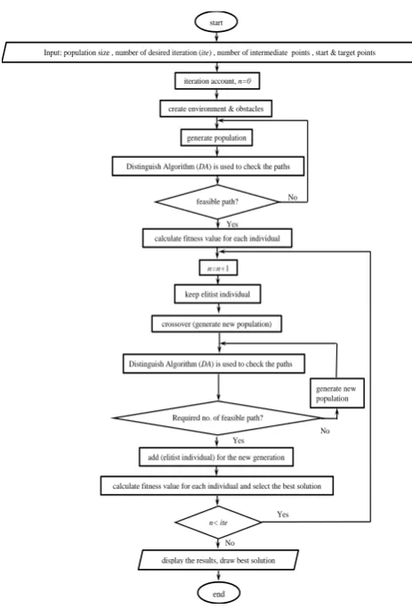
Fig 1: Flowchart of the Modified Genetic Algorithm*

The process of modified genetic algorithm is illustrated in the following steps:

3.1

Creating the Environment, and

Obstacles in the Algorithm

To verify the effectiveness of the MGA*, the simulation has been applied for different grid settings and different number of obstacles. Different known working environments are used, which are presented in Figure 2 to Figure 3. As displayed in the figures, the blue grids represent obstacle free areas where mobile robot can move freely. There is no unit used to measure the path length because each cell in the environments can represent any unit. The circle sign in the environment is the robot’s starting and goal location. The grid size, the coordinate of the start and target points, and the number of obstacles for each environment are shown in Table 1.

Table 1: Grid size, start and target point, number of obstacles

As the number of obstacles increases, the algorithm needs more generations to find the best solution. Obstacle areas in the working environment are represented by blue squares which contain red grid and has an average area of 1 × 1 unit. Boundaries for obstacles area are formed by their actual boundaries plus a safety distance that is defined with consideration to the size of the mobile robot which is treated as a point in the environment. In each environment the obstacles are randomly put but carefully placed in such a way that they keep some distance from the starting point to the target point to make sure that the robot has some space to move.

Fig 2: First working environment

Fig 3: Second working environment

3.2

Generating the Initial Population in the

Algorithm

All individuals of the initial population are assumed to be generated randomly. This leads to generate large numbers of infeasible paths which intersect an obstacle, and infeasible paths should be avoided. If there is/are obstacle(s) either in the vertical direction or horizontal direction, the mobile robot has to keep itself away from the obstacles.

Initial population stored in a single matrix of size c × m, where c is the number of individuals in the population and m is the length of the individuals. Each row corresponds to a particular solution. After generating the initial population, and

start

Input: population size , number of desired iteration (ite) , number of intermediate points , start & target points $&and target points point

create environment & obstacles

calculate fitness value for each individual

n=n+1

keep elitist individual

crossover (generate new population)

display the results, draw best solution

end generate population

feasible path?

Yes No

Required no. of feasible path?

Yes

No

add (elitist individual) for the new generation

n< ite Yes

No

generate new population iteration account, n=0

Distinguish Algorithm (DA) is used to check the paths

calculate fitness value for each individual and select the best solution Distinguish Algorithm (DA) is used to check the paths

Environments grid size [unit]

Start point [unit]

target point [unit]

number of obstacles

1st environment 31 × 23 x=1 , y=1

x=22 ,

y=30 76

2nd environment 20 × 20 x=1 , y=1

x=7 ,

y=6 94

to allow the robot to move between its current and final configurations without any collision within the surrounding environment, each individual must be checked whether it intersects an obstacle or not, as explained in the next step.

3.3

Distinguish Algorithm (DA)

Because there are both feasible path and infeasible path in the population, the Distinguish Algorithm (DA) is used to check the paths, whether the path is feasible or not, in order to come out with all feasible individuals in the population. After applying this algorithm, feasible path will be used for next generation and infeasible path will be deleted.

The details of the DA are as follows [4]:

a. Generate the line equation of a(x1, y1) and b(x2, y2)

by

:

(1)

(2)

Then, find the intermediate points between point a to point b, when the value of x is increase with 0.5. For each intermediate point, substitute the corresponding x value in equation3-2 and calculate the y value.

b. Check if the coordinate of the intermediate point lies within the obstacle area or obstacle free area by checking the particular intermediate point and obstacle list.

c. If the particular intermediate point lies within obstacle free area, repeat Step 2 until all intermediate points between point a and point b are explored. In case where any of the intermediate points lies inside obstacle area, DA is terminated and that particular path will be categorized as infeasible path.

d. If none of the intermediate points lie in the obstacle area, Step 1 to Step 3 are repeated until all points in the particular path are explored. This explored path is categorized as feasible path

.

3.4

Fitness Function

The length of the feasible path is compute as:

(3)

is the distance between two points, xi and yi are robot’s

current horizontal and vertical positions, xi+1 and yi+1 are

robot’s next horizontal and vertical positions. The objective function of the overall path can be expressed as:

where dist(j) is the distance of the jth path in the environment,

and h is the number of links that consist the path.

The fitness function is the inverse of the total distance which is Euclidean distance. The Euclidean distance between starting and target point is the length of the line segment

connecting them. The fitness function used in this thesis is (Yun et al., 2010):

where F(j) is the fitness function and j represents the jth path.

It is obvious that the best individual will have the maximum fitness value. At each generation, iteration, all the chromosomes will be updated by their fitness.

3.5

Elitism

In order to keep the best chromosome from each generation, the elitism method is employed. In elitism it is obvious that the best individual will have maximum fitness value. The main goal of the elitism rule is to keep the best chromosome from the current generation. Thus, under this rule, the best chromosome from each generation will not undergo any mutation or crossover event and will safely move to the next generation. Since the best or elite member between generations is never lost, the performance of GA can significantly be improved.

The remaining chromosomes are then sorted according to their fitness. Since small population sizes lose diversity very fast, therefore in the proposed algorithm no selection operator is used, and all the remaining chromosomes will be selected to undergo the crossover operator. Using this approach will increase the expectation of maintaining diversity in the population.

3.6

Crossover Operator

After selection of the elite member, crossover operator stage starts. In crossover a group of chromosomes undergoes crossover at each generation. All the crossover events are controlled by a certain crossover probability Pc, which is

equal to 0.5. The algorithm creates a random number in range [0 1] for each chromosome. If the generated number is less than Pc, the chromosome is a candidate for the crossover event,otherwise the chromosome proceed without crossover. The left most genes and the right most genes will avoid the crossover event since these two points are the start and target points and cannot be eliminated. For the purpose of diversity, the crossover point is randomly selected in each generation. Single-point crossover operator is used in proposed algorithm. The genes of two parents’ individuals before or after the crossover point are swapped, then the individual of the father replaced by individual of the offspring. Finally, the DA is used to check the paths of the newly generated offsprings. There is no mutation operator in the proposed MGA*. After crossover operator has been applied to the initial population, a new population will be formed.

3.7

Generation Algorithm

Genetic algorithm is terminated when the maximum number of iteration exceeds a certain limit, and also terminated when it does not find a path from the start point to the target point.

4.

MODIFIED PARTICLE SWARM

OPTIMIZATION (MPSO*)

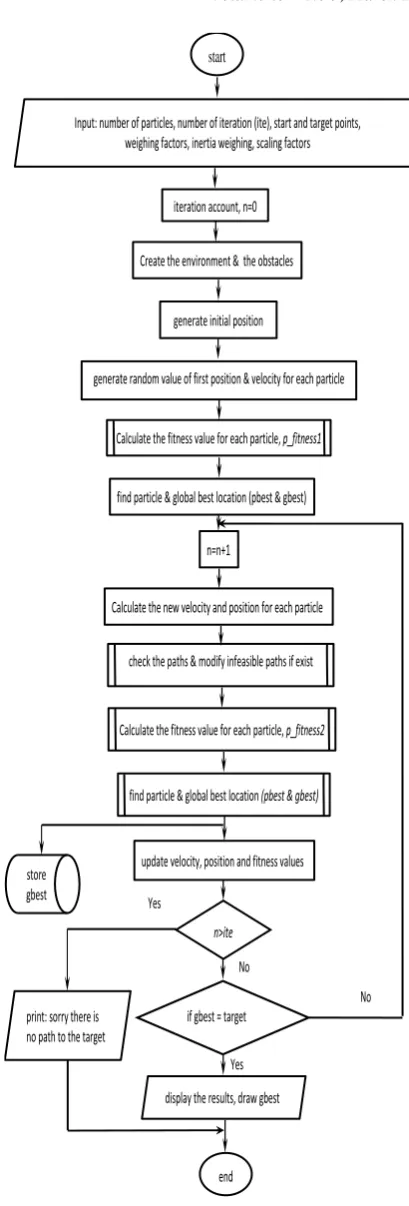
Basically the MPSO*, just like the PSO, consists of a population of particles that collectively search in the search space for the global optimum. Improvements are mainly trying to address the problem of premature convergence associated with the standard PSO. These improvements usually try to solve this problem by increasing the diversity of solutions in the swarm. In the MPSO* an error factor is modelledto ensure that the PSO converges. The MPSO* tries to address another problem which is population may include many infeasible paths which have undesirable effect on the performance of the algorithm. In the MPSO*, the infeasible paths are not discarded but can be modified to be feasible path. For example, if the particle path falls with an obstacle boundary, it is relocated to a position outside the obstacle. The process of MPSO* is demonstrated in the following subsections

4.1

Modeling the Environment, and

Obstacles in the Algorithm

The flowchart of the proposed MPSO* is illustrated in Figure 4.

Fig 4: Flowchart of the Modified Particle Swarm Optimization

4.2

Particle swarm initialization

The starting position for each particle is the starting point of the path, then the first position and velocity of each particle is generated randomly but limited to the boundaries of the search space. The particle’s position stored in a matrix with size of 2 × l, where l is the number of particles. The first and

if gbest = target

Yes No start

Input: number of particles, number of iteration (ite), start and target points, weighing factors, inertia weighing, scaling factors

generate initial position Create the environment & the obstacles

Calculate the fitness value for each particle, p_fitness1

find particle & global best location (pbest & gbest)

n=n+1

Calculate the new velocity and position for each particle

store gbest

Calculate the fitness value for each particle, p_fitness2

find particle & global best location (pbest & gbest)

update velocity, position and fitness values

display the results, draw gbest

end

generate random value of first position & velocity for each particle

check the paths & modify infeasible paths if exist iteration account, n=0

n>ite

print: sorry there is no path to the target

second row of the matrix correspond the x and y-coordinate for all particles, respectively.

4.3

Fitness Function Evaluation

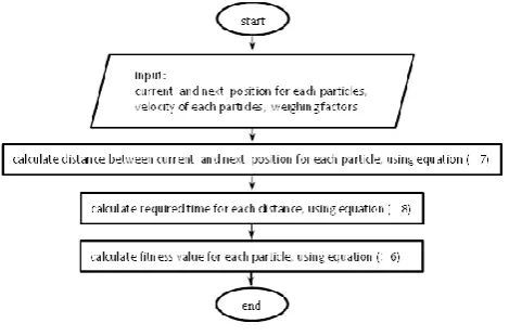
The particle’s paths are evaluated during each step. Evaluation function is used to provide a measure of how particles have performed in the problem domain. In the MPSO*, two parameters, the distance between points and travel time, indicated by the particles are used to calculate the particle fitness (p_fitness). Since the fitness should increase as the distance and time decrease, the fitness function for each particle of a feasible path is turned out to be a minimization problem and it is evaluated as:

(6)

where and are weighing factor for distance and travel time respectively, denotes Euclidean distance between point to the next point for the same particle and denotes time taken by the particle to cover from to :

(7)

(8)

where xi and yi are particle’s current horizontal and vertical

positions, xi+1 and yi+1 are particle’s next horizontal and

vertical positions, and denotes the velocity of the particle when traveling from to . The calculation of the fitness value is illustrated by the flowchart shown in Figure 5.

Fig 5: Flowchart for fitness calculation

4.4

Particle position and velocity update

The MPSO* algorithm is initialized with a number of particles and then searches for optimal. The position of a particle is influenced by the best position visited by itself which is referred to as particle best “pbest”, and the best position in the whole swarm which is referred to as a global best “gbest”. A particle updates its position and velocity using the following equations [14]:

where the cognitive component, , represents the particle's own experience as to where the best solution is and the social component, represents the belief of the entire swarm as to where the best solution is. Both and are the updated particle’s velocity , , x1 and y1 are current particle’s velocity and position along x and y-direction respectively. Updating velocities is the way that enables the particle to search around its individual best position and global best position.

Self-confidence factor, and swarm-confidence factor, makes particles have the function of self-summary and learn to the best of the swarm, and get close to the best position of its own as well as within the swarm.

The inertia weight (w) was first introduced by [15]. This term serves as a memory of previous velocities and it employed to control the impact of the previous velocity on the current velocity .The value of inertia factor (w) is in the range of [0 1]. and are random numbers within the interval of [0 1]. These parameters have considerable effects on performance of PSO.

In the basic concept of PSO algorithm no error model is used for updating the position. However, in the MPSO* these errors are modelled to ensure that the PSO converges, the modified position update equation for each particle with the error is determined as follow:

(11)

(12)

where x2 and y2 are the updated positions along x and y-direction, is a random number, large values of this parameter leads to global search, while small values leads to fine and local search which is suitable when algorithm converges. and are position error along x and y-coordinate for all particles, respectively, and it’s between current particle position and the target position. These errors are used to change the particle’s direction to head toward the target.

(13)

(14)

The error value is determined for each particle where & are the current coordinates of the individual particle and & are the target coordinates. Based on the above equations, the next possible velocity and position of each particle is determined. If the next possible position resides within the obstacle space, the obstacle avoidance part of the algorithm is employed and the Distinguish Algorithm (DA) is used to check the paths.

4.5

Generation of Feasible Paths

illustrated by the flowchart in Figure 6. As shown in the figure, if the particle path falls with an obstacle boundary, it is relocated to a position outside of the obstacle.

Fig 6: Flowchart for modifying the infeasible paths position

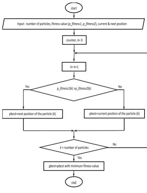
As the next step, the particle’s fitness value is compared between current and new location at each iteration to determine the best position pbest for each particle, and the particle with the best fitness value is assigned as the global best gbest, as illustrated by the flowchart shown in Figure 7.

Fig 7: Flowchart for finding the particle and global best location

The MPSO* algorithm has a main nested loop terminated when the total number of iterations exceeds a certain limit or solution convergence; otherwise the program is terminated when the program could not find the path from start position to the target position. The path generated by MPSO* is a group of “gbest” points, including start and target points. In all cases, an optimal path is formed by line segment which is connecting the global best position “gbest” falling on the grids of the working environment.

5.

SIMULATION RESULTS

The simulation results of mobile robot path planning using Modified Genetic Algorithm (MGA*) and Modified Particle Swarm Optimization (MPSO*) are presented to find the optimal path along the obstacle-free directions.To illustrate its wide applicability and their effectiveness, the proposed algorithms are implemented to solve the path planning problem through the computer simulation for different working environments. For comparison and validation purpose, the results obtained from the MPSO* algorithm are compared with results obtained by MGA*. The programs are written by MATLAB R2012a and run on a computer with 2.5 GHz Intel Core i5 and 6 GB RAM.

5.1

The Implementation of Modified Genetic

Algorithm (

MGA*

) in Path Planning

The implementation of the MGA* to solve path planning problem is demonstrated to different types of working environments. These environments are large in size and complex which have been presented to test the performance of this algorithm to find the optimal or near optimal path with satisfied time. For the proposed algorithm the simulation parameters are set as: population size =100, crossover probability (Pc = 0.5). In all cases, an optimal path is formed

p_fitness1(k) >p_fitness2(k)

No start

Input: number of particles, fitness value (p_fitness1, p_fitness2), current & next position

end counter, k= 0

Yes

pbest=next position of the particle (k)

k= k+1

pbest=current position of the particle (k)

k > number of particles

Yes

No

by line segments which are connecting the points falling on the grids of the working environment.

5.1.1

Implementation of MGA* for the First

Environment

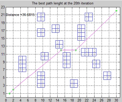
The performance of the MGA* is tested by applying this algorithm to find the optimal or near optimal path for the 1st environment shown in Figure (2). As illustrated in the figure, this working environment is a very complex environment. The best results obtained from the implementation of the MGA* are shown in table 1, and the best path found is illustrated by Figure (7) to Figure (12).

Table 1: The simulation results for the 1th environment using MGA*

Simulation Results Initial

Population

Iterations Distance Elapsed time [s]

100 20 36.6815 14.0

100 10 36.7174 9.5

100 5 37.9303 5.63

100 3 38.6729 4.5

100 2 38.9300 4.4

100 1 39.4776 3.0

The best solution obtained by MGA* shown that the elapsed time is 5.63 seconds to find shortest generated path with the length of 37.9303. However, the length of the path for 10 and 20 iterations is a bit shorter than 5 iterations but the computation time is much larger. From these results, one can concluded that, the required time to find optimal path is small.

Fig 7: Path generated for the 1st environment using MGA* (20 iterations)

Fig 8: Path generated for the 1st environment using MGA* (10 iterations)

Fig 10: Path generated for the 1st environment using MGA* (3 iterations)

Fig 11: Path generated for the 1st environment using MGA* (2 iterations)

Fig 12: Path generated for the 1st environment using MGA* (1 iteration)

5.1.2

Implementation of MGA* for the Second

Environment

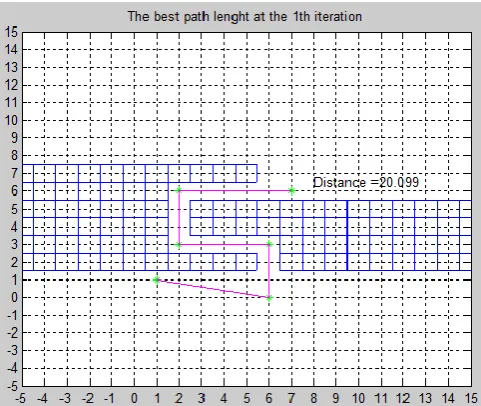
The performance of the MGA* is examined by applying a simulation for the 2nd environment as illustrated in Figure 3 . The best simulations obtained by applying the MGA* to the 2nd environment are shown in Table 2, and also the best path obtained is illustrated by Figure 13 and Figure 14.

Table 2: The simulation results for the 2th environment using MGA*

Simulation Results Initial

Population Iterations Distance Elapsed time [s]

100 2 19 67.76

100 1 20.099 44.10

Based on this result, it can be concluded that, the global optimal path obtained by the MGA* is the optimal solution.

Fig 13: Path generated for the 2nd environment using MGA* (2 iterations)

5.1.3

Implementation of MGA* for the Third

Environment (Closed Environments)

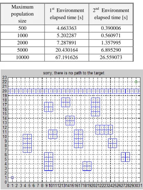
In order to show that the algorithm does not converge when there is no path to the target; the algorithm has been implemented to the two previous environments which turned to closed environments. Table 3 shows the elapsed time for the closed environments with different number of population size. For the environments the elapsed time is increased by increasing the number of population gradually because the large number of population requires larger computations.

Table 3: The simulation results for the 3th environment using MGA*

Maximum population

size

1st Environment elapsed time [s]

2nd Environment elapsed time [s]

500 4.663363 0.390006

1000 5.202287 0.560971

2000 7.287891 1.357995

5000 20.430164 6.895290

10000 67.191626 26.559073

Fig 15: First closed environment using MGA*

Fig 16: Second closed environment using MGA*

The simulation results shown in Figure 15 and Figure 16. The Figures show that if the MGA* could not find a path between the start point and the target point for the five working environments, an error message is returned so that the mobile robot could not find the target.

5.2

The Implementation of Modified

Particle Swarm Optimization (

MPSO*

)

in Path Planning

To study the performance of the MPSO*, the proposed algorithm have been applied to different types of working environments presented from Figure 2 to Figure 3. To investigate the effect of different swarm size on the performance of the MPSO*, different number of particles has been taking into account (i.e., 5, 10, 50, and 100). The particle’s size has been selected on the base of trial and error, because there has been no recommendation in the literature regarding swarm size in PSO.

In the MPSO* various combinations of parameters were tested and the best obtained result are the values of weighing factors in fitness function and , inertia weighing factor . The swarms with small initial inertia weight converged relatively fast at the beginning of optimization. The chosen values of cognitive scaling and social scaling factors are . Usually equals and ranges from 0 to 4 (Raja and Pugazhenthi, 2009).

5.2.1

Implementation of MPSO* for the First

Environment

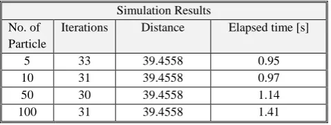
Table 5: The simulation results for the 1st _environment using MPSO*

Simulation Results No. of

Particle

Iterations Distance Elapsed time [s]

5 33 39.4558 0.95

10 31 39.4558 0.97

50 30 39.4558 1.14

100 31 39.4558 1.41

The best solution obtained after running the MPSO* algorithm to this environment is shown in Figure 17 to Figure 20.

Fig 17: Path generated for the 1st environment using MPSO* (5 particles)

Fig 18: Path generated for the 1st environment using MPSO* (10 particles)

Fig 19: Path generated for the 1st environment using MPSO* (50 particles)

Fig 20: Path generated for the 1st environment using MPSO* (100 particles)

It can be observed from the above figures that no improvement is achieved for more than 5 particles in term of the path length; therefore 5 particles are sufficient to find the optimal path with length of 39.4558 in 0.95 second.

5.2.2

Implementation of MPSO* for the Second

Environment

Table 5: The simulation results for the 2nd environment using MPSO*

Simulation Results No. of

Particle

Iterations Distance Elapsed time [s]

2 26 27 1.19

3 29 25 1.23

5 20 23 1.25

7 23 21 1.35

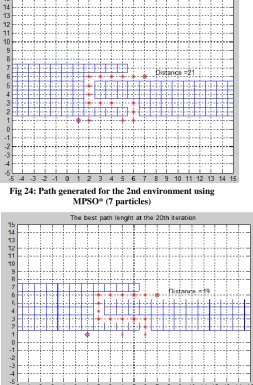
10 20 19 1.41

Fig 21: Path generated for the 2nd environment using MPSO* (2 particles)

Fig 22: Path generated for the 2nd environment using MPSO* (3 particles)

Fig 23: Path generated for the 2nd environment using MPSO* (5 particles)

Fig 24: Path generated for the 2nd environment using MPSO* (7 particles)

This algorithm has been examined with various swarm size to investigate the behavior of MPSO* algorithm in each case. This will also help in showing that MPSO* algorithm will converge to the optimal solution, optimal path, in each run. Through the simulation results, it is shown that the MPSO* can find out an optimal path very quickly.

5.2.3

Implementation of MPSO* for the Third

Environment (Closed Environments)

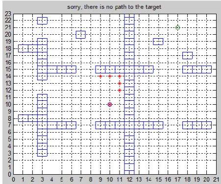
The MPSO* algorithm has been carried out to the five previous environments which turned to closed environments, in order to demonstrate that the proposed algorithm does not converge when there is no path to the target Table 6. shows the elapsed time for the five closed environments with various number of particles and different number of iterations. As shown in the table, for all closed environments the elapsed time is increased by increasing the number of particles and the number of iterations because of that the large number of particle and iteration require larger computations.

Table 6: The simulation results for the 3rd environment using MPSO*

No. of Particle 1st Environment Elapsed time

[sec]

2nd Environment Elapsed time

[sec]

10 iteration

5 0.567463 0.348209

10 0.624700 0.350721

50 0.661831 0.674306

100 0.682113 0.946107

50 iteration

5 0.639178 0.385743

10 0.696363 0.578581

50 1.223272 1.856159

100 1.636615 2.946691

100 iteration

5 0.669309 0.460107

10 0.753709 0.709233

50 1.656838 2.655063

100 2.893451 3.499064

The results illustrated in Figure 26 to Figure 30 showed that if the proposed algorithm could not find a path between the start point and the target point for the five working environments an error message is returned. In all cases, the MPSO* algorithm succeeded to avoid the obstacle, even a collision free path did not exist in the closed environments.

Fig 26: First closed environment using MPSO*

Fig 27: Second closed environment using MPSO*

Fig 29: Fourth closed environment using MPSO*

Fig 30: Fifth closed environment using MPSO*

5.3

Comparative Study between MGA* and

MPSO*

This section describes comparison results between the MGA* and the MPSO*. The achieved simulation results of both algorithms for path length and travel time for the five working environments are shown in Table 7 and Table 8, respectively. The results showed the performance of the proposed algorithms to find a feasible path for a mobile robot to move from a starting point to the target point in static environments. Results of these simulations are very encouraging and they indicate important contributions to the areas of path planning in mobile robots.

Table 7: Comparison of path length between MGA* and MPSO*

1st Environment 2nd Environment

MGA* 37.9303 19

MPSO* 39.4558 19

Diff1 1.5255 0

Diff1= path length (MPSO*) - path length (MGA*)

Table 8: Comparison of calculation time [second] between MGA* and MPSO*

4th Environment 5th Environment

MGA* 5.63 67.76

MPSO* 0.95 1.41

Diff2 4.68 66.35

Diff2= travel time (MGA*) - travel time (MPSO*)

6.

CONCLUSIONS

From the simulation results one can conclude that the proposed algorithms, MGA* and MPSO*, are capable of effectively guiding a robot moving from start position to the goal position in different working environments and find optimal/shortest path without colliding any obstacle in the environments. Also the simulation results show that the MGA* and the MPSO* algorithms have the capability of finding global optimum path in complex environment which is clearly observed in the first environment. The using adaptive population size without selection and mutation operators in the proposed MGA* led to improve the execution time. Adaptive population size grows depending on the size, structure and the number of obstacles in the environment which led to improve the execution time. In the MPSO* an error factor is modeled to ensure that the PSO converges. These errors are used to change the particle’s direction to head toward the target. A modified procedure carried out in the MPSO* to solve the infeasible path problem. When the particle path falls with an obstacle boundary, it is relocated to a position outside of the obstacle. The results obtained from the implementation of the MGA* and the MPSO* to find the optimal path for mobile robot show that the MGA* is more efficient than the MPSO* in term of minimizing distance, while the MPSO* is more efficient than the MGA* in terms of minimizing the execution time.The MGA* and the MPSO* algorithms didn’t converge in the closed environments in which there is no path between the start point and the target, as observed in the closed environment. However, the MPSO* is faster to discover that the environment is closed. The MPSO* can rightfully be regarded as a good choice due to its convergence speed and robustness in global search

7.

REFERENCES

[1] Patnaik, S., Jain, L. C., Tzafestas, S. G., Resconi,

G., Konar, A. 2005 Innovations in RobotMobility and

Control, Springer, Netherlands.

[2] Kolski, S. 2007. Mobile Robots Perception and

Navigation, Advanced Robotic Systems International and pro literatur Verlag, Germany.

[3] Han, K. M., 2007. Collision free path planning

algorithms for robot navigationproblem, Master Thesis,

University of Missouri-Columbia.

[4] Yun, S.C., Ganapathy, V., Chong, L.O. 2010. Improved

genetic algorithms based optimum path planning for

mobile robot, International Conference on Control,

[5] Mohanty, P. K., and Parhi D. R. 2013, Controlling the Motion of an Autonomous Mobile Robot Using Various

Techniques: a Review, Journal of Advance Mechanical

Engineering, Vol. 1: pp.24-39.

[6] Dutta, S., 2010. Obstacle Avoidance of Mobile Robot

using PSO-based Neuro Fuzzy Technique, International

Journal of Computer Science and Engineering, Vol. 2, Issue, (2): pp. 301-304.

[7] Tamilselvi, D., shalinie, M., Hariharasudan. 2011.

Optimal Path Selection for Mobile Robot Navigation

Using Genetic Algorithm”, International Journal of

Computer Science Issues, Vol. 8, Issue, (4): pp.433-440.

[8] Ragavan, S.V., Ponnambalam, S.G., Sumero, C. 2011.

Waypoint-based Path Planner for Mobile Robot

Navigation Using PSO and GA-AIS”, Recent Advances in

Intelligent Computational Systems (RAICS), pp. 756-760

[9] Raja, P., Pugazhenthi, S. 2012 .Optimal path planning of

mobile robots: A review, International Journal of

Physical Sciences, Vol. 7, Issue, (9): pp. 1314 – 1320

[10]Ahmadzadeh, S., Ghanavati, M. 2012. Navigation of

Mobile Robot Using the PSO Particle Swarm

Optimization, Journal of Academic and Applied Studies

(JAAS), Vol. 2, Issue, (1): pp. 32-38.

[11]Habeeb, Z. Q., 2012. A Simulation for Optimal Path

Planning for Mobile Robot Using Modified Genetic Algorithm, Master Thesis, University of Baghdad.

[12]Yu-qin, W., Xiao-peng, Y. 2012. Research for the Robot

Path Planning Control Strategy Based on the Immune

Particle Swarm Optimization Algorithm, 2nd

International Conference on Intelligent System Design and Engineering Application, pp. 724-727.

[13]Gigras, Y., Gupta, K. 2012. Artificial Intelligence in

Robot Path Planning”, International Journal of Soft

Computing and Engineering (IJSCE), Vol. 2, Issue, (2): pp.471-474.

[14]Jatmiko, W., Sekiyama K., and Fukuda, T. 2006.

Modified Particle Swarm Robotic for Odor Source

Localization in Dynamic Environment, the International

Journal of Intelligent Control and Systems: Special Issue on Swarm Robotic, Vol. 11, Issue, (3): pp.176-184.

[15]Eberhart, R., and Shi, Y. 1998. Comparison between

Genetic Algorithms and Particle Swarm Optimization.