Modified Evolutionary Autonomous Agents Approach to Image Feature Extraction

Modified Evolutionary Autonomous Agents

Approach to Image Feature Extraction

Nalin Goel

Department of Computer Engineering

Indian Institute of Technology (Banaras Hindu University),

Varanasi

K.K. Shukla

Department of Computer Engineering

Indian Institute of Technology (Banaras Hindu University),

Varanasi

ABSTRACT

In this paper, we present a modified evolutionary autonomous agents method for extracting features from a grey scale image. Features can be extracted on the basis of differences in intensity values of the target pixel with the neighboring pixels. We use agents to identify such change in the intensity values with the neighborhood. Agents are single unit entity with the power of computation and behaviors. The agent possess behaviors such as Self-reproduction, Diffusion and Death. Self-reproduction occurs when the parent agent detects the feature lying beneath it. Self-reproduction results in generation of other agents. Diffusion to another pixel occurs in case the former condition is not met until the agent attains certain age and it finally Dies. Self-reproduction and diffusion occurs in the direction governed by the previous state of the agent. Agents are independent entities hence the power of parallelizability can be really advantageous.

General Terms

Image Feature Extraction, evolutionary computation.

Keywords

evolutionary agents, feature extraction, agent behaviours, self-reproduction, diffusion, death.

1.

INTRODUCTION

Feature extraction has always been the challenging task in image processing. Edge detection is one of the fundamental tool in the field of feature extraction [1]. Edges are the organized set of points at which the image brightness changes drastically. Discontinuity in the brightness can be a result of one of the following reasons: discontinuities in depth, surface orientation, change in scene illumination and variation in material properties [2][3]. When edge detection in done on an image then ideally we get a connected curves forming the boundaries of the objects in the image. Due to this, edge detection can reduce subsequent efforts in removing the irrelevant objects in the image before proceeding further. If the edge detection is successful then the subsequent task of analyzing the image becomes easier. But like always there are many issues with this process of feature extraction. The images can be of different complexities making it difficult to solve the boundary problem. Also each time the edge detection algorithm is executed, the probability that we get the required result may not be always true. Edge detection process can result in getting false edges and the task of refining these false results can be troublesome [4].

Edge detection can be non-trivial task. It is because not always the change in intensities that depict boundaries are sharp. Edge can consist of a set of points in which the intensities are gradually decreasing. This can create problem in detecting the sharp boundaries of the objects in the image. Hence to specify a certain threshold for difference between two neighboring points is not always easy [4].

Canny edge detection is a famous answer to edge detection. His basic attempt was to derive an optimal smoothing filter on the basis of detection, localization and minimizing multiple responses to a single edge. Optimal filter to these assumptions is sum of four exponential terms [5]. Other methods in the field of edge detection includes: Gabor filter, Hough transforms, Prewitt operator, Sobel operator, etc. All of these methods are broadly classified into search-based and zero-crossing based methods. Mathematical methods uses first-order and second-first-order derivative approaches for edge detection [3].

Along with these mathematical methods of detecting edges, there exists other unorthodox approaches that not only helps in edge detection but also in detection of other feature extractions. These approaches includes computing the strength of edge or gradient magnitude and then using thresholding techniques to simplify the edges.

1.1

Related work

Previously a lot of work has been done using evolutionary autonomous agents. Evolutionary computation has remained a topic of concern for applying computation models using evolutionary process [10]. Evolutionary processes use real-life behavioral functionalities of the identities to solve certain problem domain. The motivation for this paper has been taken from the work of Jiming Liu, Y. Y. Tang, and Y. C. Cao [6].

2.

EVOLUTIONARY

AUTONOMOUS

AGENTS

During the detailed study of the algorithm proposed by Jiming Liu, Y. Y. Tang, and Y. C. Cao, it was observed that the directional self-reproduction and diffusion of the agents using the probability vectors didn’t give much speed up of the algorithm. The main reason being computation of the direction is highly dependent on the directions of the sibling, parent and grandparent agents. To understand better let us first have an overview of the method stated in [6] and then finally realizing a major possible modification that lead to better results.

The grey-scale image is considered as 2-D lattice in which pixels have distinct intensity values. We spray several agents on this lattice that can compute features using the grey-level intensities and further process their behaviors ( explained later). A distinct feature can be extracted using intensity value differences with respect to the neighbors using

(1)

Where, k = radius of the agent neighbors

I (i,j) = intensity of the pixel at (i,j)

= threshold value.

This value Dij is called local stimulus of the pixel. Then we define a range [u,v] where u is the lower range and v is the upper range. If the value of Dij (local stimulus) falls between this ranges then the feature is said to be found out. Now comes the role of behavior of the agent. If the feature is detected the self-reproduction of the agent occurs else diffusion occurs. This phenomenon occurs until agent has reached to certain age when it finally dies.

2.1

Self-Reproduction

Self-reproduction is the unique behaviour of the agent that leads to feature extraction in the image. When an acceptable local stimulus value satisfies the range [u,v] then asexual reproduction of the agent occurs. Before this asexual self-reproduction, feature markers are used to show the feature found. Infact, the agent itself converts into a feature marker. After this, the agent sprays out other agents in its neighbourhood. This can occur either in random manner or in directional manner. Random manner is simply spraying the child agents around the parent agents in any of the direction. In directional manner, we reproduce a limited amount of

agents in a direction based on the best fitted fitness function value of certain agents (to be later specified in section 2.3).

2.2

Diffusion

Diffusion occurs when the local stimulus value fails to fall in the range [u,v]. This means the underlying pixel is not a feature pixel and now this overlying agent must be diffused to another pixel in the neighbourhood. This diffusion can occur in again 2 modes: random or directional manner. In random, any of the direction can be randomly chosen. In direction, we diffuse the agent in a direction based on the best fitted fitness function value of certain agents (to be later specified in section 2.3). The length of the diffusion must range in [1, limit] where limit is the maximum permissible value of the diffusion.

2.3

Directional probability vectors

Both in case of self-reproduction and diffusion, we can choose the direction using some best fitted fitness function value. Fitness function can be defined by the following equation:

(2)

First of all, we assume that we have different generation of agents. Let there be grandparent agent belonging to g-1 generation. This grandparent generates a set of parent agents

in g generation. Finally the parent agents of this g generation generates set of g+1 generation child agents . We need to specify the directional probability

vector for a specific child agent . Well this depends upon the fitness values of the sibling agents in g+1 generation along with all the parent agents in g generation belonging to same grandparent existing in g-1 generation. We have probabilities associated with each directions, and , for diffusion and self-reproduction respectively. We select the best probability value from the direction vectors and perform the behavioural action in that direction only. This can be computed as:

1) Select all the agents belongs to {g} and {g+1} generation such that the fitness function value F( ) of the agent is greater than zero.

2) For all the selected agents in the above step, we compute for all the directions:

Where, = the set of all possible direction in which agents can diffuse.

= the set of all possible direction in which agents can reproduce.

The direction associated to best probability value is selected.

2.4

Death

After few diffusions, if the agent is unable to find the feature, then it must die. The reason is that the agent may be lying in the area where there is no feature in its vicinity, so it would not be advisable to spent CPU cycles with that agent.

3.

MODIFIED EVOLUTIONARY

AUTONOMOUS AGENTS

In this section, we present some of the short coming of the previous method and then propose a new modified version of the algorithm.

3.1

Shortcomings of previous method

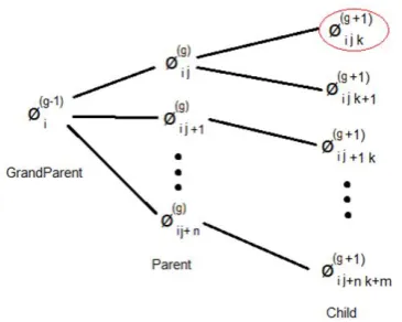
We can take a simple example to understand how sometimes, the above method of directional diffusion and reproduction can be unsuitable. In figure 1, we see the relationship between different generations of agents.

Figure 1: Relationship graph of the 3 generations of the agents.

The agent circled in red is our target agent and for this agent we need to find the directional vector in case of self-reproduction and diffusion. According to 2.3, the directional vector is dependent on all the agents in parent generation and child generation. Let us take the next example that uses this relationship graph.

In figure 2, there exists a grandparent agent at the starting point. Grandparent agent diffuses in the north direction until it comes to the edge of the grey rectangle. As soon as it detects a boundary having difference in intensities,

it self-reproduces two parent agents and in west

and north directions respectively. These two parent agents also resides on the boundary therefore self-reproduction is triggered again producing (child of ),

(child of )and (child of ) in west, north and

north directions respectively. The red circled agent

still lies on the boundary and need to self-reproduce. The

direction of this self-reproduction will be based on the agents in same generation and in the parent generation. From the figure, we see that there are 3 north directions and 1 west direction associated to sibling and parent agents. According to the equations in section 2.3, the probability of directional vector suggests north direction for the child of which is

inappropriate. Instead of north, the more suitable option is west where there exists a boundary. Hence we see that totally relying on the relationship graph can lead to unsuitable results some of the time.

Figure 2: Example figure.

3.2

Modified

evolutionary

autonomous

agent technique

This technique is a modification on the technique depicted in section 2. Section 3.1, clearly explains the shorting of the previous method in some particular cases. We propose a better technique to this problem. Instead of relying on the relationship graph, we rely on the immediate parent agent’s direction. We use a greedy algorithmic approach because features are locally important but not globally. This means that 2 child agents in g+1 generation might not be working on the same feature as in figure 2. Relying on only parent agent not only solves the above problem but also decrease the cost of updating of probability vectors of all the agents. Imagine the reduction in CPU cycles that were used while calculating and updating probability vectors in case of hundreds of agents working at the same time in the 2-D lattice.

According to the modified technique, we self-reproduce 5 child agents from the parent agent in the direction of parent agent and around that parent direction. For example, if parent agent was diffused/reproduced from north direction, then it will self-reproduce 5 child agents in the direction: north, north-west, north-east, east and west. We have fixed the number of reproducing contrary to the previous approach.

the agent discovers boundary of any of the rectangles, then that rectangle will be processed until all the features are extracted. This results in fast discovery of objects. This feature can be useful in many of the feature extraction techniques where segments are to be detected as soon as possible. In method [6], all the agents were given equal priorities because of which fast detection of any of the objects is not possible. Most of the segments are detected at the end of the feature extraction process.

Further, the general observation was that all the agents are independent in nature. Independency of the program component results in better parallelizability. We parallel the agents in a multi-core environment to make this technique better and better. This independency was not possible in the previous method because of complex relationship graph. In the modified technique, agents doesn’t depend on any relationship with sibling and parent generation agents hence the opportunity for speed up. It was observed that modified evolutionary autonomous agents on i7-2670QM processor (4 cores, 2 threads per core) yielded a speed up of ~4. Hence the already optimised method becomes faster using parallelizability.

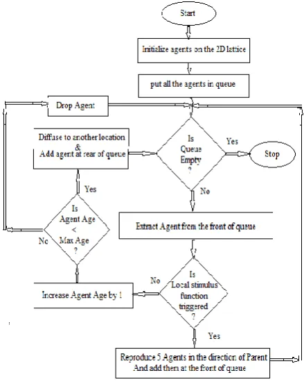
We will see in next section, few examples along with analysis of the speed up of the evolutionary autonomous agent technique.

Figure 3: Algorithm Flowchart

4.

EXPERIMENTS

Figure 3, presents a series of snapshots showing the feature extraction of a 50 x 50 grey-scaled image. In each snapshot we see the incremental feature extraction in the image. Here modified evolutionary autonomous agents technique has been used hence we see fast object detection

Figure 4: Experiment 1, red agents depics active agents and blue agents are the feature markers (a) is the initial image in which feature extraction has to be performed. (b) Initially a certain number of agents are sprayed on the 2D lattice of the image randomly, (c) gradually all the boundaries are extracted by this method, Self-reproduction occurs when a boundary is

Figure 5: Graph for experiment 2, the graph shows the number of active agents at a particular time step for different techniques. The lower line graph shows the results from modified evolutionary autonomous agent method (giving the best result), the second one is the line graph of probability vector or directional approach and

the above one (taking the most time) is the random technique

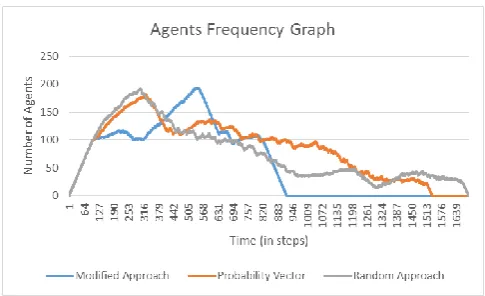
Analysis of the above experiment gave the following graph shown in Figure 4. Agent Frequency graph is a plot of number of agents to the time value. We can clearly see the huge difference between the three curves. The lower curve (most optimised) is modified evolutionary autonomous agent method. Just above it, is the curve from directional self-reproduction/diffusion method. The worst curve is from the random self-reproduction/diffusion method. Please note that the time shown here is in the number of steps but not seconds. CPU can process as many steps as possible within computation time. Parallel processors can speed up these steps.

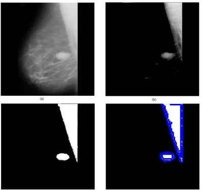
We perform another experiment shown in figure 5. The figure shows a mammography of a breast [9]. The aim is to find the tumour in the breast which can also be a breast cancer. We apply some basic gradient and thresholding tools to prepare the image for feature extraction. Then noise filtering is done. After all these pre-processing steps, modified evolutionary autonomous agent method is used to extract the features. As seen we get two objects. One of them is the tumour and another one is some imaging error. Then we also present the analysis of experiment 2.

Figure 6: Experiment 2, (a) shows the mammography of a breast, (b) gradient and thresholding tools are used, (c) Binary masking is done along with noise filtering, (d) feature extraction is done using

Figure 7: Graph for experiment 2, the graph shows the number of active agents at a particular time step for different techniques. The lower line graph shows the results from modified evolutionary autonomous agent method (giving the best result), the second one is the line graph of probability vector or directional approach and

the above one (taking the most time) is the random technique.

5.

CONCLUSION

This paper presented a modified version of evolutionary autonomous agent methods for feature extraction. With this method, we got several advantages as:

1) Fast detection of the objects in the image. This approach can be used for real-time detection of objects as in above shown case of medical image. Fast detection of objects is really important in case of security vigilance. Fast detection can also be used in manufacturing industries. 2) Independent agents resulted in parallelism which

increased the speed up.

In future, this method can be modified to communicating agent method. In such method, all the agents communicate with each other resulting in better feature extraction. But at the same time, the cost of communication will also arise. Along with it, parallelism will also be compromised. Hence it still remains a topic of research.

6.

ACKNOWLEDGMENTS

The authors wishes to thank Jiming Liu, Y. Y. Tang, and Y. C. Cao because of whom this research was possible. The authors would also like to thank fellow colleagues and the anonymous reviewers. A special thanks to MIAS database for providing precious medical data.

7.

REFERENCES

[1] Important definitions:

http://en.wikipedia.org/wiki/Edge_detection

[2] H.G. Barrow and J.M. Tenenbaum (1981) "Interpreting line drawings as three-dimensional surfaces", Artificial Intelligence, vol 17, issues 1-3, pages 75-116

[3] Lindeberg, Tony (2001), "Edge detection", in Hazewinkel, Michiel, Encyclopedia of Mathematics, Springer, ISBN 978-1-55608-010-4

[4] T. Lindeberg (1998) "Edge detection and ridge detection with automatic scale selection", International Journal of Computer Vision, 30, 2, pages 117--154.

[5] J. Canny (1986) "A computational approach to edge detection", IEEE Trans. Pattern Analysis and Machine Intelligence, vol 8, pages 679-714.

[6] Jiming Liu,Member, IEEE, Y. Y. Tang, Senior Member, IEEE, and Y. C. Cao (1997) “An Evolutionary Autonomous Agents Approach to Image Feature Extraction”, IEEE TRANSACTIONS ON EVOLUTIONARY COMPUTATION, VOL. 1, NO. 2, JULY 1997, pages 141-158.

[7] Important definitions:

http://en.wikipedia.org/wiki/Feature_extraction

[8] Definition of evolutionary agents:

http://studentreader.com/evolutionary-agents/

[9] Medical database:

http://peipa.essex.ac.uk/info/mias.html

[10] W. Banzhaf and F. H. Eeckman, Eds. (1995), “Evolution and Biocomputa-tion: Computational Models of Evolution.” Berlin, Germany: Springer-Verlag, 1995.

[11] L.J.Fogel, P. J. Angeline, and T. Back, Eds. (1996), “Proc. Evolutionary Programming” V. Cambridge, MA: MIT Press, 1996.

[12] D. E. Goldberg (1989), “Genetic Algorithms in Search, Optimization, and Ma-chine Learning”. Reading, MA: Addison-Wesley, 1989.

[13] J. Holland (1975), “Adaptation in Natural and Artificial Systems” Ann Arbor,MI: Univ. of Michigan Press, 1975.

[14] J. R. Koza (1992), “Genetic Programming: On the Programming of Computers by Means of Natural Selection.” Cambridge, MA: MIT Press, 1992.