Growth and inequalities of height in Brazil (1939 1981)

Munich Personal RePEc Archive

Growth and inequalities of height in

Brazil (1939-1981)

Monasterio, Leonardo M and Noguerol, Luiz Paulo and

Shikida, Claudio Djissey

1 June 2006

Online at

https://mpra.ub.uni-muenchen.de/1118/

TEXTO PARA DISCUSSÃO N

16

GROWTH AND INEQUALITIES OF HEIGHT IN BRAZIL (1939-1981)

Leonardo M. Monasterio (UFPel) Luiz Paulo Nogueról (UFRGS) Cláudio D. Shikida (EG-FJP - IBMEC)

GROWTH AND INEQUALITIES OF HEIGHT IN BRAZIL (1939-1981)

Leonardo M. Monasterio

Department of Geography and Economics

Federal University of Pelotas

[email protected]

+55 53 3278-6665

Luiz Paulo Ferreira Nogueról

Department of Economics

Universidade Federal do Rio Grande do Sul

[email protected]

+55 51 3316-4164

Claudio Djissey Shikida

Professor Paulo Neves de Carvalho School of Government

João Pinheiro Foundation and

Department of Economics – IBMEC/[email protected]

SUMMARY:

This paper analyzes the heights of Brazilian people using anthropometric and economic data. The literature suggests that height is a good proxy of the material living conditions of different populations. Data indicate that the difference between the heights of 21 and 65-year-old men is approximately six centimetres. The same value, by coincidence, represents the difference in the stature of the poorest and richest quintiles. Adjusted data show an increase of 3.8 centimetres in the heights of adult male Brazilians born between 1939 and 1981. There are also stable regional differences; in the North

and Northeast of the country, heights are about two centimetres lower than the national average for all groups. Regression analyses show that proxy variables related to living conditions during bodily growth, and using regional dummies, were statistically significant causes of the variation in the heights of individuals. In contrast, colour, urban/rural, and inequality variables were not significant. The results replicate what the historiography of the relation between living conditions and stature makes clear: the social environment has a significant impact on the average height of populations.

Key words:

Anthropometrics – Inequality – Indicators of conditions of life – Height - Brazil

INTRODUCTION

Inequality within Brazilian society is present in various dimensions. Income is

concentrated both regionally and individually. While part of the population enjoys living standards

and patterns of consumption comparable to those of developed countries, there are large numbers of

families living in poverty. About one third of the population lives below the poverty line, according

to official data and criteria. The poorest 20% account for 1.5% per cent of total national income,

while the richest 20% account for 68%. By comparing data from different states, we find that the

difference in life expectancy between the richest states and the poorest ones is more than eight years. Per capita income in the poorest region is equal to one fourth of that observed in the Southeast, the richest region of the country (PNUD, 2003).

The recent publication of research including anthropometric data concerning the

circles. Some researchers have concluded that the Pesquisa de Orçamentos Familiares1 2002-2003

(IBGE, 2005; henceforth POF) showed that obesity was a more serious problem than malnutrition.

In fact, the data do suggest that, even among the population in the lower strata, excess weight or

obesity is more common than weight deficit. In these strata, 24 per cent of men were overweight or

obese, while only 4.5 per cent had a weight deficit. Other analysts therefore assumed that

differences in nutrition among the various classes had disappeared in Brazil. However, some of

those who were most involved in anti-hunger campaigns mistrusted the validity of the results

presented by the IBGE2. This paper argues that the emphasis on excess weight is only one of the

interpretations which can be made of the POF data. When we change the focus to the height of

Brazilians, we can verify that, in spite of the social improvements which took place during the twentieth century, there is a long way to go before the country reaches more acceptable patterns of

equality.

When the objective is to evaluate the quality of nutrition and the living conditions of

populations, both in a wide sense and in the long term, the average stature of individuals is an excellent synthetic index. It reflects not only the average income of society as a whole, but also the

degree of access to food, together with the body’s consumption of energy, work and other physical

activities, plus the influence of diseases, especially during childhood.

Six centimetres - this paper shows that this is the approximate difference of height

between 21 and 65-year-old Brazilians, and coincidentally between adults in the richest and the poorest quintiles of the population. Contrary to common belief, the literature notes that genetic differences, despite their individual impact, are unimportant when we consider all individuals in

terms of stature. In any given population, there are tall and short individuals, but their average

height can be determined by external conditions, that is, through genes and the environment. In the

case of whole populations, however, living conditions are the most important factor. Thus, in adulthood, height is bound up with both nutrition and health, a trait which would be difficult to

Economic historians such as Richard Steckel (1982, 1995), John Komlos (1989) and

Robert Fogel (2004) were the first to collaborate in the creation of this research field. The heights

of American Indians and slaves, eighteenth-century German aristocrats, and military personnel from

a range of countries, have been analyzed by these academics and their co-authors. They have shown how the heights of individuals have varied, at different periods and in different locations,

while linking these variations with present-day living conditions.

Since there are no long-term data available on the evolution of the height of Brazilians,

this paper uses the POF data to evaluate evolution and inequality within this dimension.

Considering that height reflects the conditions in which populations used to live, and not current

conditions, it would be ideal if there were data available on the families of the adults who were

interviewed by the IBGE. Since this information is not available, other analytical strategies have

had to be implemented. On the basis of cross-section data, proxies have been used to estimate those

aspects of living conditions which have had an influence on the average stature of the adult

Brazilian population. In order to estimate the effects of this, regression analysis has been carried

out3.

This paper contributes to a new interpretation of the IBGE’s POF data: the height of most

Brazilians is below its potential because existing living conditions are far from satisfactory. Even

when we consider the progressive reduction in malnutrition, the existence of basic sanitation in most Brazilian urban areas, and the debate about the need for education on nutrition (which shows

that part of the population does not have problems of malnutrition, but problems relating to a

low-quality diet), there are still significant inequalities regarding access to health and general sanitation

services, and to income. All these factors are reflected in the differences of height among

Brazilians, taking into account the different geographic regions and the disparities in income, as

verified in this paper. We would therefore like to reiterate the importance of using anthropometrics

in evaluating the results of social and economic policies, rather than using just the traditional

HEIGHT AND LIVING CONDITIONS: A SUMMARY

The energy generated by the consumption of food can be divided into two categories: one

is for the maintenance of vital functions, and the other is a reservoir of energy for physical

activities, especially work. When nourishment is inadequate for these, there is also a “third

demand”, caused by related diseases, that is, a variety of diseases which tend to reduce the body’s

ability to absorb the nutrients ingested. In this case, without an improvement in nourishment, the

individual, besides being exposed to a life-threatening risk, becomes temporarily incapable of

working, since there is no energy left over for corporeal activities except those necessary for

baseline maintenance4.

Throughout history, human beings have had a wide range of dietary patterns. These patterns reflect not only “cultural preferences”, but also the access of populations to food, which is

conditioned by a constant interactive process between income and wealth. A. Sen (1999, p. 204)

gives an example of this process when he writes about the Irish famines. The English officials

tended to blame the Irish themselves and their eating habits for the calamity they were experiencing.

According to Sen, this reflected the lack of understanding and the cultural distance between the two

countries5. In fact, the heavy consumption of potatoes in Ireland was more the result of poverty

than of choice.

In Europe and the United States, the relevant literature emphasized not only the process

of the increase in the height of populations in the twentieth century, but also the occurrence of

cycles. The average American in the mid-eighteenth century was taller than in the mid-nineteenth

century, and both were shorter than in the twentieth century. However, per capita income in the

United States did not follow similar cycles. It increased continuously over the period in question,

correlation between per capita income and height, this correlation is not always a direct one.

Likewise, from the eighteenth to the twentieth century there was a similar cycle in England, even

though the average Englishman was shorter than the average American. In other countries, such as

Norway, there was a continuous process of increase in the average height of the population. The

inhabitants of the United States, who were taller than all Europeans from the eighteenth century to

the 1950s, were then overtaken by the average Dutchman and Scandinavian.

One of the interpretations for the height cycle phenomenon in several populations,

according to which nineteenth-century men were shorter than eighteenth and twentieth-century

men, is that, higher income levels due to the Industrial Revolution did not compensate for urban

living costs, the variation in the relative prices of foodstuffs, long journeys to and from the place of

work (which also applied to women and children), and insalubrious living conditions in industrial

centres. This situation was later mitigated by social legislation, investments in health and

education, basic sanitation, treatment of drinking water, and other improvements.

In support of the arguments relating to income and to the harsh living conditions faced by

workers during the Industrial Revolution, Robert Fogel (2004, p. 40) states that the difference in

height between rich and poor English people was 12 centimetres in the nineteenth century, and this

was associated with marked differences in terms of life expectancy and income. The same situation

pertained in other European countries, such as Germany and France. As time went by, the increase

in the overall level of income, relatively greater among the poor than among the rich, and the creation of social welfare institutions, led to a decrease in the difference in height between the two

categories. In England today, the difference in height between people of higher and lower income

is only 2.5 centimetres. This difference has disappeared completely in Sweden and in the

The increase in income of Americans between 1875 and 1995, for example, led to a substantial relative decrease in expenditure on nutrition, clothing and shelter. This indicates that

people were able to purchase the essential goods for the satisfaction of these needs, which

correlates strongly with the stature of the population. It was also an opportunity for the creation of

other needs and wants. In the nineteenth century, expenditure relating to the three items mentioned

above absorbed 74 per cent of the budget of American families, but only 13 per cent at the end of

the twentieth century (Fogel, 2004, p. 89).

If there are no nutritional restrictions, there is likely to be intensive growth during the

early years and adolescence. Girls tend to conclude this process of growth before boys. After these

two periods of maturation, the speed of growth tends to decrease until it stabilizes. When there is

an event that seriously restricts good nutrition, the increase in height tends to cease during this period, but a certain recovery is likely to occur later, in a new phase of nutritional plenty.

As an example of this, the case of American slaves, as outlined by Steckel (1995, p. 1924), is worthy of note. During childhood, the slaves suffered serious nutritional restrictions and

were prey to diseases caused by the conditions of slavery, and the lack of knowledge of simple

hygiene. The maternity leave granted to slave women was too short to allow adequate

breastfeeding, which apparently ended when the child was 3 months old. Moreover, the high

density of children living in the same environment and using the same eating utensils greatly

facilitated infection by microbes, which caused, for example, diarrhoea, measles and chickenpox.

The effects of nutritional deficiencies on growth, given the difficulties imposed on breastfeeding,

and of the lack of hygiene in childhood are evidenced by the fact that slave children can be found in

the lowest centiles of height in present-day growth charts. As adolescents, the American slaves

were fed better and, it seems, they recovered part of the growth deficit that had taken place in the

There istherefore abundant international evidence linking the average height of

populations to their past and present living conditions. It is clear that increases in per capita

income, better income distribution, and positive social policies in general have beneficial effects on

the height of individuals.

EMPIRICAL EVIDENCE

Steckel (1995, p. 1906) argues that height can be an excellent index of quality of life and

development, following the agenda proposed by A. Sen (1999, chapter 2) concerning lifestyles.

Stature measures performance by health history rather than inputs to

health, which has the advantage of incorporating the supply of inputs

to health as well as demands on those inputs...

Gilberto Freyre, the renowned Brazilian sociologist, in Casa Grande e Senzala, which

is required reading for the study of slavery , tells that he was inspired to write the book when, on

travelling to the United States in the 1920’s, he realized that Afro-Americans were visibly taller

than Afro-Brazilians6. According to Freyre, this difference was less due to climatic and racial

factors (at that time considered essential in determining individual characteristics) than to the

different social regimes to which populations with similar origins were subject7.

The empirical evidence collected and put forward by Steckel (1995, p. 1910)

corroborates Freyre’s view:

Africa (or of European or African descent), and from India or the Middle East, have similar growth profiles.

On the basis of other sources, Steckel states:

Although tropical climates have a bad reputation for diseases, Maurice King (1966) argues that poor health in developing countries is largely a consequence of poverty rather than climate. A group of diseases are spread by vectors that need a warm climate, but poverty is responsible for the lack of doctors, nurses, drugs, and equipment to combat these and other diseases. Poverty, via malnutrition, increases the susceptibility to disease (Steckel, 1995, p. 1911).

According to Steckel (1995) and Fogel (2004), the height of different peoples tended to

increase during the twentieth century as a result of improvements in the environments where they

lived. These environmental improvements should be understood in a broader sense, as is the case

with development for Sen (1999), that is, they should include not only those which result from a

higher income level that allows people to feed themselves better, but also those which result from

public policies which mitigate people’s exposure to infectious agents, such as adequate sanitary inspection of food, treatment of water, and efficient garbage and sewage collection.

Steckel (1995, p. 1912) argues that, although the correlation index between average height and per capita income varies from 0.82 to 0.87, it is necessary to consider other factors,

such as income distribution. The Gini Coefficient is negatively related to average height in the

populations analyzed (Steckel, 1995, p. 1914), that is, the worse the income distribution in a

particular country, the lower the average height. Concentration of income reduces stature for two

obvious reasons: low-income people constitute the majority of the population, and they will have

the greatest difficulty in accessing through the market the necessary nutrients to satisfy their

genetic potential.

In addition to this, healthcare also correlates positively with levels of income. Diseases

are responsible for “nutrient waste”, since a sick person tends to have more difficulty in absorbing

them. Thus, low income and high susceptibility to pathogenic factors combine to reduce the height

Still on the subject of social environment and health, in addition to considerations of

income, the article by Komlos and Baur (2004) may be quoted in respect to the following enigma.

The American population, in the eighteenth and nineteenth centuries, and for a great part of the

twentieth century, was one of the tallest in the world. At present, besides being relatively tall,

Americans, differently from continental Europeans, have a high obesity index. The average

American Body Mass Index (weight divided by height squared, hereafter referred to as BMI) is

very high, which in tall populations also means a high average weight. Komlos and Baur argue

that the American BMI reflects the lack of social welfare mechanisms that exist in most Western

European countries. Specifically, the lack of comprehensive health assistance and unemployment

insurance exposes children to temporarily insufficient nutrition (thus compromising their growth)

and to unsatisfactory medical care. As attested by the authors, the effect on Americans’ health is

evident: compared with Europeans, who have a lower per capita income, Americans have a lower

life expectancy rate and a higher child mortality rate.

D

This work is based almost exclusively on POF microdata. In addition, Brazilian

population censuses of the twentieth century, estimates of each state’s participation in Brazilian GDP (Azzoni, 1997), and IPEA8 GDP data for the period between 1939 and 1981, were used to

estimate per capita income by state during this period. The research considered only POF

microdata related to men who, at the time they were interviewed, were between 21 and 65 years old.

This was done in order that the data would be comparable to data from other research9. After the

INCREASES IN HEIGHT

It is a well-known fact that there has been a trend of increased growth in Brazilians in the

most recent cohorts. Graph 1 demonstrates the evolution of this trend. The average height of people who were born in 1940 was about 1.65 m, whereas it was almost 1.71 m for cohorts studied

at the beginning of the 1980s. This represents an increase of almost 1.5 cm per decade, but though

it is a substantial increase, even larger ones have been recorded. In the Netherlands between 1900

and 1950, the average height of adults increased from 1.69 m to 1.78 m (Steckel, 1995, p. 1919).

This trade-off between height and age, in a cross-section study, must be cautiously

analyzed. Individuals tend to lose height from the age of 40 onwards. Although bones do not

diminish in length, changes in vertebrae, intervertebrate discs, standing positions and foot curvature

tend to aggravate height loss. The intensity of the loss depends on several factors; physical activity

and nourishment seem to be the main determinants (MedlinePlus, 2005). In order to adjust the POF

data, we have used the height correction proposed by Niewenweg et al (2003), based on data on the

Dutch population in the twentieth century. This procedure involves adding to the current height of

an A-year-old individual ( A21) the following expression: _0,042_(A₂₁₎_[0,0015_(A_21)]2_.

The adjusted series, presented as a dotted line in Graph 1, shows that the increase in the height of

Brazilians during the period was about 3.8 cm, and not 6 cm, as was previously supposed.

Basing his hypothesis on extensive literature, Fogel (2004, p. 23) asserts that shorter

individuals tend to have lower life expectancy rates. The same factors which are responsible for

rates of growth below their potential can cause more delicate conditions of health later in life. In

the present case, this means that shorter individuals tend to be absent in the higher age ranges of the

sample. It is therefore likely that, if the data were adjusted for different mortality rates, the actual

GRAPH 1 – AVERAGE HEIGHT VARIATION IN CM BY COHORT BETWEEN 1938 AND 1982

SOURCE: AUTHORS BASED ON POF. NOTE: TRIENNIAL MOVING AVERAGES.

It is important to note that Brazilians who were born in 1981 had, at the beginning of the

21st century, an average height (170.8 cm) similar to Americans and Norwegians (171 cm), but below that of the Swedes (172 cm), and above that of the British (167 cm), Dutch (169 cm) and

French (165cm) at the beginning of the twentieth century.

R

The analysis of the evolution of aggregated data omits important regional and income

differences. Graph 2 below represents the differences between regional and national average height

in Brazil. People living in the south of the country, whatever the cohort, tend to be three or more

centimetres taller than those from other regions. People living in the centre-west and south-eastern

regions tend to be similar in height, and are about two centimetres above the average. On the other 165

166 167 168 169 170 171

1940 1943 1946 1949 1952 1955 1958 1961 1964 1967 1970 1973 1976 1979 1982

hand, the stature of people living in the north and north-eastern regions tends to be two centimetres

below the average. The most noticeable fact is that, despite the increase in Brazilian average height, people living in the north and north-eastern regions do not converge to this average. This

suggests that the persisting socio-economic differences which exist between the Brazilian regions

are reflected in the anthropometric data.

Unfortunately, the data used here do not provide information about migration. Thus, we

only have information about the individual’s current place of residence, and not on the place where

he/she grew up. At first, this would seem to be a serious distortion, because there were substantial

internal migratory movements in the decades analyzed, especially from the Northeast to the

Southeast. However, since migration tends to occur towards richer locations, this distortion tends to

inaccurately reduce – and not increase – regional differences. In other words, height differences

between Northern and North-eastern populations, in comparison with South-eastern, Southern and

GRAPH 2 - REGIONAL DIFFERENCES, IN CENTIMETERS, CONCERNING BRAZILIAN AVERAGE HEIGHT BY COHORT – 1938-1982

SOURCE: AUTHORS BASED ON POF. NOTE: TRIENNIAL MOVING AVERAGES.

H

,

The last row in Table 1 shows that 6 cm is the difference in height between the poorest

and the richest quintiles10. If, as these data demonstrate, this difference has persisted since the 1930s, we can say that, contrary to the pattern in rich countries, in Brazil there was a process of

economic growth which benefited the population as a whole (since the quintile average height increased), but unevenly, and not favourably to the poor. Hence there has been no tendency

towards the suppression of height differences between rich and poor people in all the regions of the

country, or even between regions. In other words, policies for reducing regional inequalities were

incapable of eliminating them. In fact, the current average height of a 21-year-old Northern and

North-eastern inhabitant is near the (adjusted) stature of Brazilians born in 1940. -5

-4 -3 -2 -1 0 1 2 3 4 5

1940 1943 1946 1949 1952 1955 1958 1961 1964 1967 1970 1973 1976 1979 1982

It is therefore evident that part of the regional difference in height is due to regional differences in living conditions. When individuals are divided into quintiles by region, and their

heights are examined, an interesting picture appears. Differences in regional stature persist in each

income quintile. Northern residents in the richest quintile, for example, are about 3.6 cm shorter

than Southern residents in the same quintile. As for the poorest quintile, the difference is as much

as 5 cm.

TABLE 1 – AVERAGE HEIGHTS BY MACRORREGION AND PER CAPITA FAMILY INCOME QUINTILE Region _Poorest

Quintile 2

nd _Poorest

Quintile

Intermediate Quintile

2nd Richest Quintile

Richest Quintile

Total

North 165.15 165.95 167.06 168.15 170.28 167.06 Northeast 165.44 166.40 167.29 168.87 170.95 167.12 Center-W est 168.40 169.05 170.34 171.40 172.95 170.72 Southeast 168.71 169.09 170.15 171.02 172.91 170.95 South 170.04 169.84 170.67 172.21 173.82 171.96 Total 166.09 167.36 168.80 170.35 172.35 168.99 SOURCE: AUTHORS BASED ON POF.

H

,

In POF, individuals were classified as belonging to the following ethnic groups or

colours: yellow, white, Brazilian Indian, brown or black. The issue of discrimination or prejudice

caused by race or colour is particularly complex in Brazil, and will not be discussed in this paper.

Since the 16th century, identification by race in Brazil has been carried out in accordance with physical and social aspects, especially in terms of the categories Brazilian Indian, black, white and

brown. Consequently, it is possible that a brown or Brazilian Indian person will be considered

white if rich, and black if poor. In the same way, it is possible that a rich person who is categorized

as white becomes poor, and from then on is considered brown. It is worth noticing that, if the

criterion for African descent is 10 per cent of African ancestry which is reflected in certain genetic

categories are problematic, we use them because we do not want to dismiss a priori either the possibility of differences in height related to colour or race, or the aggregate of information made

available in the database.

The data tabulated by income quintile and colour also furnish interesting results. If we

observe average heights only by reference to colour, we could say that colour is the main

determining factor of height. White men are the tallest, followed by black, yellow, brown and Brazilian Indian. However, when the results are analyzed by quintile, we can see that:

Brazilian Indian people are the shortest in the three lowest height strati; 

Yellow people are the shortest in the richer strati;

White people are the tallest in the two poorest quintiles and in the richest quintile;

Black people are the tallest in the intermediate and in the second richest quintiles.

These changes in order are due to a different distribution by colour when we consider

income quintiles. In the richest quintile, there are 29 per cent white, but only 13.5 per cent black,

and 12.6 per cent brown. Therefore, a significant part of the apparent height variation by colour is

in fact a result of the differences in income distribution between the colours, and not within the

TABLE 2 – AVERAGE HEIGHT BY COLOR AND PER CAPITA FAMILY INCOME QUINTILE Poorest

Quintile

2nd Poorest Quintile

Intermediate Quintile

2nd Richest Quintile

Richest Quintile

Total

Yellow Average 164.33 164.56 169.83 168.37 168.52 167.75 % of total colour 11.39 11.39 14.56 22.15 40.51 100.00 White Average 167.12 168.35 169.64 171.18 173.03 170.51 % of total colour 11.76 15.49 19.54 23.72 29.49 100.00 Brazilian

Indian

Average 162.96 160.79 165.69 170.06 170.86 164.80

% of total colour 33.12 24.84 16.56 11.46 14.01 100.00 Brown Average 165.69 166.76 167.97 169.28 171.05 167.69 % of total colour26.57 23.39 20.40 17.06 12.58 100.00 Black Average 166.47 168.28 170.09 171.21 172.74 169.38 % of total colour 23.25 24.00 20.60 18.66 13.49 100.00 Total Average 166.09 167.36 168.80 170.35 172.35 168.99 % of total colour 20.00 20.00 20.00 20.00 20.00 100.00 SOURCE: AUTHORS BASED ON POF.

T

If height is a good indicator of quality of life, it is to be expected that this indicator will

be affected by a range of socio-economic, family and environmental determinants. As mentioned

above, it would be ideal if data on those determining factors during the individual process of

physical maturation were available. Since this is not the case, we have had to consider that there is

a correlation between present and past living conditions. We have also considered that individuals

with a higher level of education, and higher per capita family income, tend to have had better

pre-adolescent living conditions. As such, height should be related to these variables. The database

used also allows us to verify common assertions about regional or colour differences which

influence the quality of life.

In order to verify our hypothesis, we started with (1):



  

 Y Y color dummies color dummies Y other controls

Height ₁₂ * (1)

Y is measured on a logarithmic scale and is divided into Y1 (variables related to family

income), and Y2 (variables related to individual human capital). The POF data only contains

income by consumption unit, that is, by family, and not per capita. In order to arrive at an estimate,

we calculated per capita family income, i.e. the total income of the consumption units divided by

basis for comparison. Other controls refer to regional dummies (South, Northeast, Centre-West and

North, with Southeast as a reference), a rural dummy and a control for age.

We acknowledge that there may be endogeneity in Y, so we postulated two alternative

forms which are intended to verify the significance of sub-vectors Y1 and Y2 separately.

          

 Y color dummies color dummies Y other controls

Height ₁ * ₁ (2)

          

 Y color dummies color dummies Y other controls

Height ₂ * ₂ (3)

Finally, we had to consider the possibility that taller individuals have higher income. This means of causality was emphasized by Schultz (2002); the hypothesis is that height is part of

the health component of human capital, and would be an indicator of individual productivity. To

control the possibility of reverse causality between height and income, a two-stage specification

was estimated. u s instrument other bY a Y controls other Y dummies color dummies color Y Height                2 1 2

1 *  (4)

R

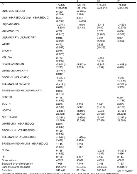
In specification (I), we noted that individuals who spent more years in school displayed

an increase in height. This effect is due to the better nutritional conditions in their homes, given

that in Brazil per capita family income in childhood is a determinant factor in people’s education.

In the colour dummies, we note that only Brazilian Indian is significant (Black is the reference

category). As for the interaction terms, there is significance only between colour and human

capital, and only for the colour Yellow. Even when we consider (II) and (III), there is little

difference between the variables which remain significant. Basically, Brazilian Indian, South,

North and Northeast remain strongly significant. In (III), White is positive and significant. The

interaction terms between human capital and colour are significant only for Yellow and Brazilian

Summarizing what has been discussed above inequalities of height among Brazilians is

basically due to income, level of education, and region. Colour alone is not a strong variable for

determining stature (except for Brazilian Indian)12. Thus, differences in height seem to be caused

by inequalities of living conditions relating to the family (reflected in income and education level),

and the wider environment where the individual lives (represented by the regional dummies).

Finally, in (IV) the endogeneity between income and human capital is considered. In this

specification we verify that the trade-off between height and income is non-linear (with increasing

returns). This result gives weight to the thesis that, as regards regional influences (three of the four

regional dummies are significant) income has a strong influence on the height of the individuals in

the sample. Influences derived from the colour of the individual appear only in Brazilian Indian

and in the income interaction effect for Brown and Brazilian Indian, demonstrating that height

increases for these groups of individuals have slightly less impact on their height.

Even when we consider the estimate made by using instrumental variables, we can argue

that the individual’s quality of life depends on factors such as income inequality or family income

during childhood. It is expected that, ceteris paribus, greater incomes have positive effects on height, although this effect is dissipated through time. On the other hand, states with higher levels

of income inequality would tend to have larger differences in height among the individuals in that

state. In terms of individual height, however, it is not possible to forecast a clearer impact (in fact,

this variable was not statistically significant in any of the specifications). In any case, this variable

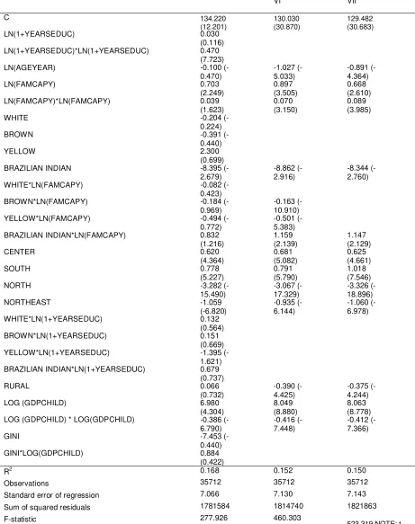
was included in the second group of regressions, numbered (V), (VI) and (VII)13.

In (V) and (VI), there is only a repetition of the procedure set out in the last table, in

which we began with the more general specification and excluded the non-significant variables.

again in an attempt to understand the relationship between human capital and income. Thus, for

purposes of comparison, only (IV) and (VII) are to be considered.

The results of the two specifications are very similar. Nonetheless, it isworth

emphasizing that GDP PER CHILD, that is, the average state GDP per capita of each individual up

to 15 years old, shows both positive and negative effects on stature. The colour dummies, in their

turn, give a result which is similar to the first group of regressions: once again, only Brazilian Indian is significant.

Estimate (VII) shows that height depends basically on economic conditions. In this

sense, we can state that individuals who grew up in relatively richer states and families had more

education, and today have both higher income and stature.

In Table 4, it is noticeable that the effect of state GDP per capita during childhood is

particularly significant when compared to other variables. In specification (VII), a hypothetical

TABLE 3 – ECONOMETRIC RESULTS – DEPENDENT VARIABLE: HEIGHT I

II IIII IV

C 172.529 (156.368) 175.148 (361.030) 176.981 (223.248) 176.805 (221.137) LN(1+YEARSEDUC) _0.1224 (0.509) -0.326 (-2.126) LN(1+YEARSEDUC)*LN(1+YEARSEDUC) 0.467 (8.108) 0.881 (16.796) LN(IDADEANO) -2.277

(-18.504) -1.610 (-13.434) -3.416 (-30.001) -3.429 (-30.270) LN(FAMCAPY) 0.762 (2.616) 0.576 (2.400) 0.868 (3.597) LN(FAMCAPY)*LN(FAMCAPY) _0.046 (2.064) 0.094 (4.483) 0.081 (3.855) WHITE 0.472 (0.547) 0.828 (10.355) BROWN 0.273 (0.325) YELLOW 2.713 (0.899) -2.169 (-4.015) BRAZILIAN INDIAN -5.804

(-2.223) -5.542 (-5.065) -2.947 (-4.399) -4.019 (-6.819) WHITE*LN(FAMCAPY) -0.172

(-0.949) BROWN*LN(FAMCAPY) _-0.320

(-1.805)

-0.230 (-7.997) YELLOW*LN(FAMCAPY) -0.412

(-0.690)

-0.567 (-5.903) BRAZILIAN INDIAN*LN(FAMCAPY) 0.063

(0.113) CENTER 0.198 (1.636) 0.214 (1.746) SOUTH 0.806 (6.102) 0.708 (5.921) 0.746 (6.210) 0.829 (6.180)

NORTH -2.836

(-22.102) -3.240 (-28.452) -2.933 (-25.638) -2.756 (-21.338) NORTHEAST _-2.341

(-21.765) -2.920 (-33.307) -2.497 (-27.898) -2.347 (-21.692) WHITE*LN(1+YEARSEDUC) 0.009 (0.042) BROWN*LN(1+YEARSEDUC) 0.120 (0.582) YELLOW*LN(1+YEARSEDUC) -1.964

(-2.430)

-1.660 (-6.496) BRAZILIAN INDIAN*LN(1+YEARSEDUC) 1.145

(1.520) 1.213 (1.851) RURAL _0.138 (1.626) -0.339 (-4.057) -0.327 (-3.886)

R2 0.160 0.147 0.142 0.144

Observations 40028 40028 40028 40028 Standard error of regression 7.096 7.149 7.168 7.163 Sum of squared residuals 2014912 2045462 2056635 2053178 F-statistic 346.441 691.244 665.748 _{561.312 NOTE:} t-Statistic in parentheses. Least Squares in regressions I, II and III. In IV, Two-Stage Least Squares. Instruments:

TABLE 4 – ECONOMETRIC RESULTS – DEPENDENT VARIABLE: HEIGHT V VI VII C 134.220 (12.201) 130.030 (30.870) 129.482 (30.683) LN(1+YEARSEDUC) 0.030 (0.116) LN(1+YEARSEDUC)*LN(1+YEARSEDUC) 0.470 (7.723) LN(AGEYEAR) -0.100

(-0.470) -1.027 (-5.033) -0.891 (-4.364) LN(FAMCAPY) 0.703 (2.249) 0.897 (3.505) 0.668 (2.610) LN(FAMCAPY)*LN(FAMCAPY) 0.039 (1.623) 0.070 (3.150) 0.089 (3.985)

WHITE -0.204

(-0.224)

BROWN -0.391

(-0.440)

YELLOW 2.300

(0.699) BRAZILIAN INDIAN -8.395

(-2.679)

-8.862 (-2.916)

-8.344 (-2.760) WHITE*LN(FAMCAPY) -0.082

(-0.423) BROWN*LN(FAMCAPY) -0.184

(-0.969)

-0.163 (-10.910) YELLOW*LN(FAMCAPY) -0.494

(-0.772)

-0.501 (-5.383) BRAZILIAN INDIAN*LN(FAMCAPY) 0.832

(1.216) 1.159 (2.139) 1.147 (2.129) CENTER 0.620 (4.364) 0.681 (5.082) 0.625 (4.661) SOUTH 0.778 (5.227) 0.791 (5.790) 1.018 (7.546)

NORTH -3.282

(-15.490) -3.067 (-17.329) -3.326 (-18.896) NORTHEAST -1.059 (-6.820) -0.935 (-6.144) -1.060 (-6.978) WHITE*LN(1+YEARSEDUC) 0.132 (0.564) BROWN*LN(1+YEARSEDUC) 0.151 (0.669) YELLOW*LN(1+YEARSEDUC) -1.395

(-1.621) BRAZILIAN INDIAN*LN(1+YEARSEDUC) 0.679 (0.737) RURAL 0.066 (0.732) -0.390 (-4.425) -0.375 (-4.244) LOG (GDPCHILD) 6.980

(4.304)

8.049 (8.880)

8.063 (8.778) LOG (GDPCHILD) * LOG(GDPCHILD) -0.386

(-6.790)

-0.416 (-7.448)

-0.412 (-7.366)

GINI -7.453

(-0.440) GINI*LOG(GDPCHILD) 0.884 (0.422)

R2 0.168 0.152 0.150

Observations 35712 35712 35712 Standard error of regression 7.066 7.130 7.143 Sum of squared residuals 1781584 1814740 1821863 F-statistic 277.926 460.303

523.319 NOTE: t-Statistic in parentheses. Least Squares in regressions V and VI. In VII, Two-Stage Least Squares. Instruments:

CONCLUSIONS

Nowadays, agreement is almost unanimous that GDP per capita is insufficient for measuring

gains in welfare. However, more controversial is the discussion about an adequate way to

complement it. Part of the research is focused on the ‘capabilities’ approach (Sen, 1999), while

another part tries to measure directly individuals’ happiness (Frey and Stutzer, 2002). This paper

has emphasized the importance of using stature as a means of evaluating the living conditions of

different populations. This may lead to misunderstandings, but we suggest neither that the height of

individuals should be considered an aim in itself, nor that there is any kind of superiority in taller

people. We only suggest that, in situations in which it is necessary to evaluate the economic and

social needs of populations, height can be considered as a pertinent dimension.

Height differences between income strati in Brazilian society are persistent and relevant. According to Fogel (2004, p. 24), shorter people have a higher risk of mortality and are more subject to certain diseases, even when they are in social conditions similar to tall people. Therefore,

the unequal distribution of income, and of sanitation and health services, which are responsible for

the differences in height, generate an additional burden on the poorest, especially on those who

have fewest resources to purchase medication and food, and to pay for health treatment.

The data on the evolution of the height of Brazilians between 1938 and 1981 confirm a

well-known fact: in spite of the per capita increase in income over this period (3.2% a year), there was no

equivalent improvement in welfare services. However, the data referring to the cohorts born after

two ‘lost economic decades’, the height of Brazilians continued to increase, confirming that socially the years from 1981 and 2001 were not as disastrous as the evolution of income.

REFERENCES

Azzoni, C.R. (1997) Concentração regional e dispersão das rendas per capita estaduais: Análise a partir de séries históricas estaduais de PIB, 1939–1995. Estudos Econômicos , v. 27, n.3.

Davis, M. (2001) Late Victorian Holocausts: El Niño Famines and the making of the Third World. London: Verso.

Fogel, R. W. (2004) The escape from hunger and premature death, 1700-2100. Europe, America, and the Third World. Cambridge: Cambridge University Press.

Frey, B. and Stutzer, A. (2002) What can economists learn from happiness research? Journal of Economic Literature, v. 40, pp. 402-435.

Freyre, G. (1977) Casa Grande & Senzala, In: Obra Escolhida. Rio de Janeiro, Nova Aguilar.

IBGE. (2005) Pesquisa de orçamentos familiares 2002-2003– Microdados. Segunda divulgação. Brasília: IBGE.

Komlos, J. Rejoinder. (1989) Nutrition and economic development in the eighteenth-century: Habsburg monarchy: an anthropometric history. Princeton, N.J.: Princeton University Press. xvii, p. 325.

Komlos, John and Baur, Marieluise, (2004). From the tallest to (one of) the fattest: the enigmatic fate of the American population in the 20th century, Economics and Human Biology, Elsevier, vol. 2(1), pp. 57-74.

MedlinePlus. (2005) Aging changes in the bones, muscles, and joints.

http://www.nlm.nih.gov/ medlineplus/ency/article/004015.htm. As seen on 1st of June.

Niewenweg, M. L. (2003) et al. Adult height corrected for shrinking and secular trend: Annals of Human Biology, Sept.-Oct, v. 30, n. 5, pp. 563-569(7).

Pena S and Bortolini M C. (2004). Pode a genética definir quem deve se beneficiar das cotas universitárias e demais ações afirmativas? Estudos Avançados , v. 18, n.50.

Salsburg, D. (2001) The lady tasting the tea: how statistics revolutionized science in the twentieth century. New York: Henry Holt.

Schultz, T. P. (2002) Wage Gains Associated with Height as a Form of Health Human Capital. American Economic Review, v.92, n.2, Papers and Proceedings of the One Hundred Fourteenth Annual Meeting of the American Economic Association, Atlanta, GA, January 4-6, 2002, May, p.349-353.

Steckel, R. H. (1982) Height and per capita income. NBER working paper n. 880.

1

Translator’s note: Family Budget Research.

2

Translator’s note: IBGE stands for Instituto Brasileiro de Geografia e Estatística, Brazilian Institute of Geography and Statistics, which is the Federal Bureau of Statistics in Brazil.

3_{It is worth noting that the expression regression analysis comes from Francis Galton’s research on the differences in height}

between generations (see Salsburg, 2001).

4

“In France, during this era (1790) daily consumption was about 1,800 calories. A typical American male in his early thirties requires nearly 2,300 calories for baseline maintenance, and by implication the typical European of the late eighteenth century was much smaller and lighter. This evidence indicates that the diets in England and France near the end of the eighteenth century were so inadequate that approximately one-fifth of the labour was incapable of work or could do no more than three hours of light work daily”. (Steckel, 1995, p. 1925).

5

“Charles Edward Trevelyan, the head of the Treasury during the Irish famines, who saw not much wrong with British economic policy in Ireland (of which he was in charge), pointed to Irish habits as part of the explanation of the famines. Chief among the habitual failures was the tendency of the Irish poor to eat only potatoes, which made them dependent on one crop. Indeed, Trevelyan’s view of the causation of the Irish famines permitted him to link them with

his analysis of Irish cooking. ‘There is scarcely a woman of the peasant class in the West of Ireland whose culinary art exceeds the boiling of a potato’. The remark is of interest not just because it is rather rare for an Englishman to find a suitable occasion for making international criticism of culinary art. Rather, the pointing of an accusing finger at the meagerness of the diet of the Irish poor well illustrates the tendency to blame the victim. The victims, in this view, had helped themselves to a disaster, despite the best efforts of the administration in London to prevent it.” (Sen, 1999, p. 174-175).

See Davis (2001) for an overview on the participation of bureaucrats and governors in famine epidemics in the world at the end of the nineteenth century.

6

“ (...) Vi uma vez, depois de mais de três anos maciços de ausência do Brasil, um bando de marinheiros nacionais – mulatos e cafuzos – descendo não me lembro se do São Paulo ou do Minas pela neve mole do Brooklin. Deram-me a impressão de caricaturas de homens. (...) A miscigenação resultava naquilo. Faltou-me quem me dissesse então, como em 1929 Roquette Pinto aos arianistas do Congresso Brasileiro de Eugenia, que não eram simplesmente mulatos ou cafuzos os indivíduos que eu julgava representarem o Brasil, mas cafuzos e mulatos doentes.” (Freyre, 1977, p. 77). Translation: “I saw once, after three whole years away from Brazil, a group of Brazilian sailors –mulatos and cafuzos – disembarking I don’t remember whether from the São Paulo or from the Minas on the soft snow of Brooklyn. They gave me the impression of being a caricature of men. (…) Miscegenation resulted in that. Nobody told me then, like in 1929 Roquette Pinto told the aryanists in the Brazilian Congress of Eugenics, that those who I thought were Brazilians were not simply multatos or cafuzos, but ill mulatos and

cafuzos.”

Translator’s note: Mulatos are usually described as descendants of white and black people; cafuzos would have white and Brazilian Indian ancestors.

7

“ Ligam-se à monocultura latifundiária males profundos que têm comprometido, através de gerações, a robustez e a eficiência da população brasileira, cuja saúde instável, incerta capacidade de trabalho, apatia, perturbações de crescimento, tantas vezes são atribuídas à miscigenação (...) _{” (Freyre, 1977, p. 79).}

Translation: “The serious diseases that have been undermining throughout generations the strength and the efficiency of the Brazilian population, whose unstable health conditions, uncertain labour ability, apathy and growth disturbances are attributed to miscegenation, are actually linked to large-scale monoculture plantations.”

8

Translator’s note: IPEA stands for Instituto de Pesquisa Econômica Aplicada, Applied Economics Research Institute, a Brazilian governmental institution.

9

Since the largest part of historical studies is based on military databases, the analyses are mostly about men.

10_{A comparison between the two extreme deciles increases the difference to more than seven centimetres.} 11

According to Steckel (1995), people from the Far East are possibly the only case in which genes seem to matter. Nevertheless, we stress that this can be related to differences in diet. Even among the individuals of this ethnic group, per capita income and height are positively correlated.

12

The White dummy showed significance in one of the regressions (III), but – as further explained – this significance disappeared in the better-specified regressions (IV and VII).

13