A Practical Approach to the Performance Analysis of
Software Components using Calibrated Software
Reliability Growth Models
S. Charles Ilayaraja
Assistant Professor Sethu Institute of Technology,
Virdhunagar, India.
M. Ganaga Durga,
Ph.D Assistant ProfessorGovernment Arts College for Women, Sivagangai, India.
ABSTRACT
Many software tools have been proposed for the purpose of performance analysis and measurement on software executables. The results produced by such tools are visually displayed based on run-time characteristics of software executables without suggesting the fitness of executables at the operational environment. This is because run-time characteristics of an executable are not static for every running instance even in the same platform and same machine configuration. In this paper, an efficient method has been introduced to estimate fitness of software executables to the operational environment by incorporating Software Reliability Growth Models. The objective of this new method is to suggest the level of fitness of software applications based on reliability measures. For this purpose, existing reliability growth models are calibrated and run-time attributes of executables have been employed instead of failure data. The estimation of fitness at the operational environment of software executables will reduce the complexities in both performance analysis and maintenance.
KEY WORDS
Application fit, process calling structure, run-time characteristics, operational environment, instrumentation process
ACRONYM & NOTATIONS
SRGM Software Reliability Growth ModelMVF Mean Value Function
FD Function and its descendant’s time
NHPP Non Homogeneous Poisson Process
m(t) mean value function with respect to time
fm(t) mean value function with delay factor
a initial parameter estimate
b proportionality constant
min(fd) minimal function time
min(∆fd) minimal differenced function time
max(fd) maximal function time
max(∆fd)maximal differenced function time
avg(fd) average function time
avg(∆fd) average differenced function time
delay factor to be incorporated in time
1.
INTRODUCTION
The performance of executables in windows environment can be evaluated by their run-time characteristics such as time elapsed at CPU, processing time for memory profiling, function and its
Windows environment, the run process of software executables is initiated with instrumentation process and followed by memory profiling. Instrumentation is the special process of loading and executing the DLLs that are required for the successful run at the current instant of the given application [11]. The run-time characteristics of the same application (software executables that run at stand alone) at different instant are not same due to the variation in the instrumentation process at the every instant of application run. As a result of such variation, the calling structure of running application is also varying with respect to its running instance.
The calling structure that is created for an application is used to determine time elapsed at CPU for both callers and called modules and the time spent from a specific calling function to its descendants. The calling structure is represented visually as call graph where thicker edges represent the bottlenecks in the calling sequence. In call graph, nodes represent the calling module and the edges represent the calling sequence mechanism. The bottleneck or load is identified by means of the thickness of the edge. The edges having more thickness have to be resolved to tune up the application performance. Thin edges within calling structure can be achieved by optimizing three attributes: elapsed time, function and descendant time and processing time [11].
In this paper, the possibility of thin edges within calling structure is estimated using SRGMs. The mean value function generated on the three attributes can be used to suggest the fitness of application at the operational environment. The application fit is characterized by people, data, tool and environment. The values of first two attributes have been recorded by using IBM Rational Quantify and the third attribute has been recorded by using IBM Rational Purify. The observed data set have been employed on s-shaped delay SRGM model [3]. The unknown parameters of the model have been estimated using (Statistical Modeling and Estimation of Reliability Functions) SMERFS 2.0 package. The plots of mean value function and other numerical computations for each data set have been done using MATLAB 2012 environment.
1.1
Motivation
An adaptive framework has been proposed to address the difficulty in the analysis of inter-component interactions of modular software systems by incorporating path testing. This framework suggests estimating path reliability of each software component based on common programming constructs such as sequence, branching and looping and then system reliability is estimated. The work on this framework shows that the path testing has high correlation to the actual software reliability. It can be used for early stages of software development with certain assumptions [6].
Software architecture knowledge has been taken into account to assess the system reliability by considering correlated component failures. This approach is suitable for component based software applications whose dependency is high [7]. The role of residual faults in the estimation of reliability has been analyzed and a filtering approach is proposed to determine the actual fault load. By using fault injection method the residuals that are not useful for the estimation of system reliability have been ignored. This approach is effective on component based software system whose architecture is complex and components are tightly coupled [8].
The usage of generic reliability models is difficult because of the variability in the failure process. Even though many models have been proposed in the unified approach, no one is suited for all the cases. To address this problem a normalized development metrics are suggested to separate domain knowledge from the process to achieve generic predictive models [9].
The estimation of both faults and vulnerabilities on software applications helps to improve its reliability. The similarities of both fault and vulnerability prediction models have been analyzed and common metrics proposed to use both models interchangeably for the estimation of reliability [10].
1.2
Software Reliability Growth Models
Software reliability is one of the quality attributes that can be defined as the probability of failure free operation within specified period of time and operational environment. The estimation of software reliability improves the effectiveness of test process and hence the life time of the product [3]. Many SRGMs have been proposed for the estimation of reliability and they have been classified into three broad groups: error seeding models, data domain models and the time domain models. The time domain models have been widely adopted due to the usage of statistical techniques and the estimation is based on curve fitting on the observed data [1].
The models are called as growth models because the system reliability grows with respect to the time as the test progresses. Most of the SRGMs use failure data which can be obtained during test phase of software development. The estimation process begins at the proportionality constant that indicates failure rate and next at the initial number of failures at the start of testing. The estimation progresses through the specified time interval by computing cumulative number of failures [3]. Then system reliability at the specified point of time can be estimated by using
(1)
The selected SRGM is based on unified approach and allows imperfect debugging. The failure process is described by using NHPP with the necessary assumptions and unified SRGM has been defined as in [1] [2]
(2)
The generalized distribution is converted to specific distribution as two staged er-lang distribution and we obtain yamada s-shape delayed model by using certain assumptions as in [12]
(3)
1.3
Model Calibration
SRGMs can be incorporated with performance analysis and measurement on the performance of an executables by including additional parameters with respect to the characteristics of operational environment. For our experiment, two core applications and two user defined applications have been selected in 32-bit Microsoft windows environment. Each application that is running is characterized by the following run-time attributes:
1. Function and its Descendant time 2. Time elapsed at CPU
3. Processing time for memory profiling
These attributes are employed as the parameters of the existing SRGMs to estimate better calling structure of running applications [4].The selected model (3) is incorporated with a delay factor to suggest the fitness of the running application to the operational environment. The delay factor is defined as the ratio of threshold of variation in FD time to the threshold in FD time of all instances of application run. It is proposed by
(4)
Where
(5)
(6)
By using the delay factor in (3) the s-shaped model is slightly modified as
(7)
The calibrated model as in (7) is modified version of s-shape delayed model. The delay factor is observed due to the abnormal variation at some of the running instances.
The MVFs of both CPU elapsed time and memory profiling time are more practical in the calibrated model than the fundamental model because of the consideration of abnormal variation. This abnormal situation is experienced by the platform due to the problems in resource allocation and scheduling [5].
2.
DATA ANALYSES
Table 1. Time elapsed at CPU Run
# DS-I DS-II DS-III DS-IV
1 4313 657 6711 9047
2 1969 328 4719 5500
3 2078 328 4093 7844
4 2406 203 5478 4766
5 1829 297 4469 5234
6 1922 218 4953 4515
7 1984 391 4360 5500
8 1937 219 5766 7219
9 1860 938 4281 4438
10 1953 328 6875 4703
11 1844 203 6641 4188
12 1734 188 7078 3906
13 2734 312 5672 4047
14 2766 313 6093 4391
[image:3.595.318.539.176.599.2]15 2579 344 6157 4657
Table 2. Processing time for memory profiling Run
# DS-I DS-II DS-III DS-IV
1 874 374 765 561
2 702 515 436 546
3 718 561 484 687
4 515 515 546 671
5 562 405 483 514
6 764 515 452 609
7 749 343 625 499
8 734 515 499 530
9 484 374 593 562
10 499 327 593 546
11 690 296 499 483
12 687 343 671 530
13 608 390 452 687
14 530 514 687 640
15 500 359 531 686
The four data sets are described as follows
DS-I have been observed by running a text editor (notepad)within Microsoft windows operating system
DS-II have been observed by running a file system interface (explorer)within windows operating system
DS-III have been observed by running an user defined code that has been written in VC++ 6.0 with fundamental constructs: sequence, branching and looping
DS-IV have been observed by running an another user defined code that has been written in Visual C++ 6.0 with the programming constructs: sequence, branching and recursion
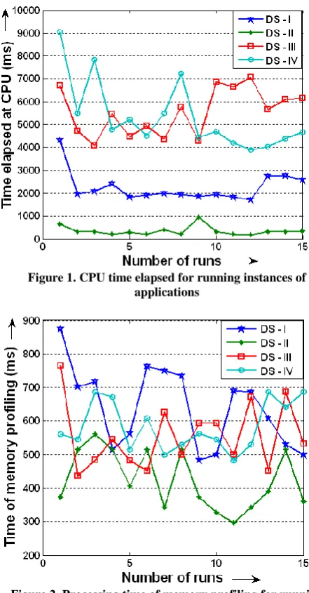
By observing Table 1 and Table 2, processing time of memory profiling has more variation than CPU elapsed time. This variation is due to the memory management policy of the
at the time of independent application run is used to record FD time. On 15 running instances, its variation is recorded by comparing its current instance with the previous instance. These observations are used to compute delay factor as in (4), (5) and (6).
The plots of four data sets for CPU elapsed time and processing time of memory profiling are presented in Fig. 1 and Fig. 2.
Figure 1. CPU time elapsed for running instances of applications
Figure 2. Processing time of memory profiling for running instances of applications
[image:3.595.80.269.324.543.2]Table 3. Estimation of parameters for both elapsed time and processing time
B a
DS-I Telapsed 0.213 40944 0.6363
Tprocess 0.214 11636
DS-II Telapsed 0.221 6246 1.2952
Tprocess 0.215 7627
DS-III Telapsed 0.165 117800 0.7294
Tprocess 0.183 10951
DS-IV Telapsed 0.254 89488 0.6466
Tprocess 0.191 11223
3.
EXPERIMENT RESULTS
The selected SRGM is one of the fundamental time domain reliability models whose reliability grows as the test process progress. The selected SRGM (3) and its calibrated version (7) are incorporated with data sets DS-I, DS-II, DS-III and DS-IV for both Telapsed and Tprocess for fifteen number of running instances of windows applications. The MVF plot for Telapsed of both SRGMs (3) and (7) for each data set is presented in Fig. 3 to Fig. 6.
Similarly the MVF plot for Tprocess of SRGMs (3) and (7) for each data set is presented in Fig. 7 to Fig. 10. When comparing plots of each MVF from Fig. 3 to Fig. 10, the cumulative time estimate is lower in calibrated SRGM model than the estimation in
fundamental model. This variation illustrates the inabilities of SRGMs to incorporate environmental factors that are influence on the estimation of reliability.
[image:4.595.319.541.108.272.2]Figure 3. Comparative plots of MVF on time elapsed at CPU for DS – I
[image:4.595.324.542.288.495.2]Figure 4. Comparative plots of MVF on time elapsed at CPU for DS – II
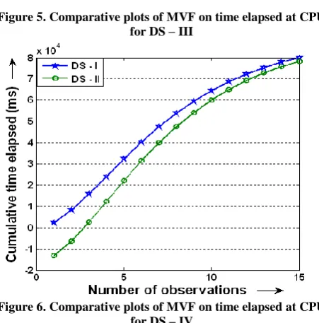
Figure 5. Comparative plots of MVF on time elapsed at CPU for DS – III
Figure 6. Comparative plots of MVF on time elapsed at CPU for DS – IV
[image:4.595.57.284.419.634.2] [image:4.595.323.549.500.729.2]Figure 7. Comparative plots of MVF on processing time of memory profiling for DS – I
[image:5.595.56.283.81.503.2]Figure 8. Comparative plots of MVF on processing time of memory profiling for DS – II
Figure 9. Comparative plots of MVF on processing time of memory profiling for DS – III
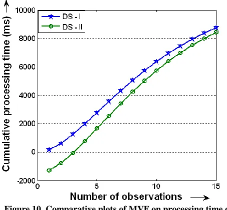
Figure 10. Comparative plots of MVF on processing time of memory profiling for DS – IV
The percentage of variation in cumulative estimate of CPU elapsed time and processing time is not more than 10% in all cases. This percentage of variation may be helpful in suggesting the fitness of software executables at the operational environment. From Table 4 and Table 5, DS-I have lowest percentage of variation and DS-II, have highest percentage. This is because of the complexity in the calling structure. It is observed that the software applications having less dependency to its running platform may have good level of fitness at the operational environment.
[image:5.595.57.282.81.289.2]Both Telapsed and Tprocess are affected by the calling structure of the specific application run. The variation is observed for all cases because of dynamic nature of calling structure of running applications at every instance. Without considering this variation, the SRGM may not estimate reliability of the application with respect to the practical environment. The difference in MVFs with and without delay factor is illustrated in Table 4 and Table 5.
Table 4. MVFs variation in CPU elapsed time estimate with θ m(t)
Without
fm(t) with
Percentage of variation
DS-I 33908 32887 3.01
DS-II 5267 4942 6.16
DS-III 83346 78940 5.29
DS-IV 79955 78253 2.13
Table 5. MVFs variation in processing time estimate with θ
m(t) Without
fm(t) with
Percentage of
variation
DS-I 9659 9371 2.98
DS-II 6346 5935 6.48
DS-III 8316 7940 4.52
DS-IV 8751 8426 3.71
[image:5.595.56.281.516.723.2]both FD time and ∆FD time have been set as in (5) and (6) to compute delay factor.
The delay factor is used to identify practical constraints on each instances of the independent application run. In practical situations, some of running instances of have maximum variation which is indicated by the threshold values. These variations are considered for achieving reliability so that an efficient calling structure can be created. This calling structure may be studied to suggest the fitness of applications within the specified operational environment.
4.
CONCLUSION
In this paper, a new method of analysis and measurement on performance of software executables was presented. Run time attributes of software executables were incorporated into SRGMs to estimate fitness of software executables within the specified operational environment. The time elapsed at CPU, processing time of memory profiling and function time, were employed as parameters of SRGMs instead of failure data as in the traditional reliability estimation. The fundamental SRGM is calibrated with a delay factor to extend practical applicability of the estimation process. The delay factor was computed by using the calling structure of executables which is obtained at the time of running instance. The MVF of selected SRGM was adjusted by means of delay factor into the exponential time scale parameter. Considerable variation was observed on both MVFs that were generated with and without delay factor. This level of variation can be used to identify the level of dependency of software executables to the running platform. The experiment results indicate that the variation between two MVFs is not more than ten percent and hence the selected executables are having 90% of fitness to the operational environment. By increasing the number of running instances of same application within same platform, the data may fit into more SRGMs and hence more dimensions may be suggested for the estimation of application fitness at the operational environment.
5.
REFERENCES
[1] P. K. Kapur, H. Pham, Sameer Anand, Kalpana Yadav, “A Unified Approach for developing Software Reliability Growth Models in the presence of Imperfect Debugging and Error Generation”, IEEE trans. on Reliability, Vol. 60, No. 1, 2011,pp:331-340
[2] Chin-Yu Huang, M.R. Lyu, Sy-yen Kuo, “A Unified Scheme of some NHPP models for Software Reliability Estimation”, IEEE trans. on Software Engineering, Vol. 29, No. 3, 2003, pp:261-269
[3] Razeef Mohd, Mohsin Nazir, “Software Reliability Growth Models: Overview and Applications”, Journal of Emerging Trends in Computing and Information Sciences, Vol. 3, No. 9, 2012, pp: 1309-1320
[4] Yonghee Shin, Robert M. Bell, Thomas J. Ostrand, and Elaine J. Weyuker, “On the Use of Calling Structure Information to improve Fault Prediction”, Emprical Software Engg., vol.17, 2012, pp.390-423
[5] Tacho kwon and Zhen dong Su, “Automatic Detection of Unsafe Dynamic Component Loadings”, IEEE trans. Software Engg., vol. 38, No.2, 2012, pp.293-313
[6] Chao Jung Hsu and Chin yu Huang, “An Adaptive Reliability Analysis using Path Testing for Complex Component based Software Systems”, IEEE trans. Reliability,Vol.60, No.1, 2011, pp.158-170
[7] Lance Fiondella, Sanguthevar Rajasekaran, and Swapna S. Gokhale, “Efficient Software Reliability Analysis with Correlated Component Failures”, IEEE trans. Reliability, vol.62, no.1, 2013, pp.244-255
[8] Roberto Natella, Domenico Cotrono, Joao A- Duraes, and Henrique S. Madeira, “On Fault Representativeness of Software Fault Injection”, IEEE trans. Software Engg., vol.39, no.1, 2013, pp. 80-96
[9] Brendan Murphy, “The Difficulties of Building Generic Reliability Models for Software”, Empirical Software Engg., vol.17, 2012, pp. 18-22
[10] Yonghee Shin, and Laurie Williams, “Can Traditional Fault Prediction Models be Used for Vulnerability Prediction?”, Empirical Software Engg., 2013, vol.18, pp.25-59
[11] Rational Suite Tutorial, IBM-Rational e-development company, April 2000, Part No: 800-023316-000, Product Version: Rational Suite 2000.02.10