Calibration of a crop model to irrigated water use using a genetic algorithm

www.hydrol-earth-syst-sci.net/13/1467/2009/ © Author(s) 2009. This work is distributed under the Creative Commons Attribution 3.0 License.

Earth System

Sciences

Calibration of a crop model to irrigated water use using

a genetic algorithm

T. Bulatewicz1, W. Jin2, S. Staggenborg2, S. Lauwo3, M. Miller1, S. Das4, D. Andresen1, J. Peterson5, D. R. Steward3, and S. M. Welch2

1_{Kansas State University, Department of Computing and Information Sciences, USA} 2_{Kansas State University, Department of Agronomy, USA}

3_{Kansas State University, Department of Civil Engineering, USA}

4_{Kansas State University, Department of Electrical and Computer Engineering, USA} 5_{Kansas State University, Department of Agricultural Economics, USA}

Received: 15 February 2009 – Published in Hydrol. Earth Syst. Sci. Discuss.: 16 March 2009 Revised: 21 July 2009 – Accepted: 3 August 2009 – Published: 14 August 2009

Abstract. Near-term consumption of groundwater for irri-gated agriculture in the High Plains Aquifer supports a dy-namic bio-socio-economic system, all parts of which will be impacted by a future transition to sustainable usage that matches natural recharge rates. Plants are the foundation of this system and so generic plant models suitable for coupling to representations of other component processes (hydrologic, economic, etc.) are key elements of needed stakeholder de-cision support systems. This study explores utilization of the Environmental Policy Integrated Climate (EPIC) model to serve in this role. Calibration required many facilities of a fully deployed decision support system: geo-referenced databases of crop (corn, sorghum, alfalfa, and soybean), soil, weather, and water-use data (4931 well-years), interfacing heterogeneous software components, and massively paral-lel processing (3.8×109model runs). Bootstrap probabil-ity distributions for ten model parameters were obtained for each crop by entropy maximization via the genetic algorithm. The relative errors in yield and water estimates based on the parameters are analyzed by crop, the level of aggregation (county- or well-level), and the degree of independence be-tween the data set used for estimation and the data being pre-dicted.

1 Introduction

Regionally, short-term consumption of groundwater in the High Plains Aquifer provides for a dynamic bio-socio-economic system through irrigated agriculture. In the long

Correspondence to: S. M. Welch ([email protected])

term, transition to sustainable usage that matches natural recharge rates will impact ecologies, economies, demograph-ics and the landscape. Recharge is that portion of precipita-tion not lost as evaporaprecipita-tion from foliage, run off (affected by ground cover), or root uptake. This problem is of global significance as National Geographic (Montaigne, 2002) de-clared the High Plains Aquifer to be one of 22 worldwide “critical areas” for “annual renewable water”.

This problem has been studied extensively from various disciplinary perspectives with disparate unaligned concepts, viewpoints, vocabulary, models and data. Stakeholder de-cision makers in this system are equally distributed across a mix of governmental agencies, administrative units, private sector enterprises, and farmers. Disjoint disciplinary science leaves these decision makers ill equipped to understand how consequences of management actions and policies impact and cascade through the integrated system. Thus, all stake-holders share a common need for integrated, science-based, quantitative informational tools that, collectively, target their differing individual responsibilities. Toward this end, re-searchers at Kansas State University, in conjunction with stakeholder groups, have begun to integrate economic, agro-nomic, and hydrologic models, supported by geodatabases, to aid in these diverse decision making processes (Steward et al., 2005, 2009a; Steward and Bernard, 2006a,b; Bernard et al., 2004, 2005; Yang et al., 2009).

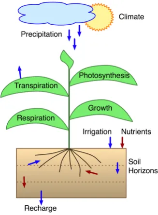
Fig. 1. Plants produce carbohydrates from carbon dioxide, water, and light energy. They grow and develop at rates that are nonlin-early dependent on resources and temperature. All but ca. one per-cent of water use is for transport or cooling and is transpired.

water fluxes and may not partition landscapes in ways di-rectly related to hydrological features or patterns of diver-sion. In contrast, physiological, parcel-based crop simula-tors, including the Environmental Policy Integrated Climate (EPIC) model1 (Sharpley and Williams, 1990; Williams et al., 1990), are well suited for linkage to other models and to Geographic Information Systems (Lal et al., 1993; Engel et al., 1997; Yang et al., 2003). Our specific objective is to es-timate irrigation needs for large numbers of representative, geo-referenced parcels. This flux couples directly to hydro-logical models. We have used Sheridan County, Kansas, as a study area to prototype this estimation process. This study evaluates the suitability of the EPIC model for providing crop simulation to decision support systems at the regional scale. In this work we chose a county size as this represents a stan-dard land unit size for aggregation of information reported about crop production (yields, etc.), information that was needed for this study. We are also evaluating extending these methods to larger scales such as the Ogallala Aquifer portion of Kansas.

The first step is to calibrate the EPIC model. Although basically a parameter estimation process, heavy computa-tional requirements mandate development of much of the infrastructure required by a fully deployed decision support system. This includes geo-referenced databases of crop, soil, weather, and water-use data, interfacing heterogeneous software components (i.e. model, optimizer, data retrieval), and, most importantly, distributed parallel processing. The

1_{Originally named the Erosion Productivity Impact Calculator.}

latter is required because benchmark runs indicated that ca-libration would require 4 to 14 d on a 40-CPU computing cluster (a significant underestimate as events later proved). On a computations-per-minute basis, this appeared represen-tative of the computing intensity required for multi-year, spa-tially distributed, water policy analyses. The following sec-tions present the elements of our calibration approach and the results obtained.

2 The EPIC model

Plant processes have been extensively modeled (Bowen, 1992; Bouman et al., 1996). The EPIC model simulates the physiology of all major forages and crops in the study area. Using a daily time step, three major processes are represented: (1) phenological development; (2) dry mat-ter production and partitioning to plant tissues, resulting in growth; and (3) economic yield. Outputs that are relevant to this study are crop yield and water use reported in t/ha and mm-ha, respectively. The model reproduces the results of irrigation, fertilization, tillage, variety selection, alternative production calendars, etc. EPIC also includes an economic component for evaluating and optimizing management out-comes. (In our research, however, a more robust economic forecasting submodel is being used (Peterson and Steward, 2006) to suggest crop management choices for EPIC to sim-ulate.) Because its original focus was erosion-related, EPIC can simulate decade-scale or longer intervals. These features have suited EPIC to a broad range of applications, including plant nutrition studies (Cole et al., 1987; Dautrebande et al., 1999); national and international assessments of agroecolog-ical change impact (Brown and Rosenberg, 1999; Brown et al., 2000; Bernardos et al., 2001), including the High Plains Aquifer (Easterling III et al., 1993); irrigation planning and water use (Bryant et al., 1992; Ellis et al., 1993; Evers et al., 1998; Guerra et al., 2005); and regional studies (Geleta et al., 1994; Cabelguenne et al., 1995; Fortin and Moon, 2000).

EPIC can be divided into nine subroutines of which hy-drology and plant growth were of interest for our simula-tions (Williams et al., 1990). The hydrology subroutine is composed of surface runoff, percolation, lateral sub-surface movement and evaporation. These processes in our simula-tions were controlled by the parameters used to describe the soil groups. Slope, and NRCS runoff curves, soil water con-tent and rainfall amounts determine runoff. Percolation and lateral sub-surface movement is controlled by the soil layer data. Potential evaporation was estimated using the Penman-Monteith method.

to as a harvest index. Species-specific parameters distinguish between crops.

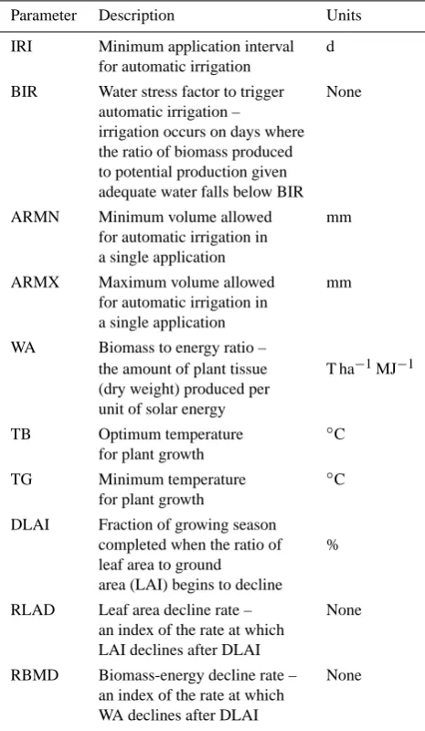
EPIC is able to simulate multiple crops because it embod-ies a generic plant model that can be re-parameterized to rep-resent different species. Table 1 describes the subset of these parameters that were estimated for four major regional crops: corn, grain sorghum, alfalfa, and soybean2. A priori param-eter value ranges are given in Table 2 – the first column con-tains values suggested in the EPIC Users Manual (Williams et al., 1990). The other columns are based on authors’ expe-rience within the study area. The former are wider because of the crop and geographic diversity of EPIC utilization. Al-though some of the chosen parameter ranges exceed the typ-ical ranges stated in the EPIC documentation, these typtyp-ical ranges do not reflect the limits that the model is capable of simulating.

Variables that control plant growth and canopy develop-ment (and subsequent water use) were selected for optimiza-tions. These were WA, TB, TG, DLAI, RLAD, and RBMD (Table 2). Variables that affect irrigation timing (IRI, BIR, ARMN, and ARMX) were also optimized. Other inputs that might affect hydrology (soil runoff curve and slope) were based on the soil groups. Growth-related parameters such as fertilizer uptake were not altered as plant nutrition was not of interest and simulations were managed in a manner such that nutrient stress did not affect plant growth and canopy development.

The irrigation-related parameters deserve special mention. The dates and amounts of individual irrigation applications are rarely available to modelers. Thus, most crop simula-tors include “automatic irrigation” options under which ir-rigations are simulated on dates when preset soil moisture or water stress levels are reached. We sought values for the parameters defining this option that reproduce annual water usage for wells in the study area – in effect attempting to solve for indexes of irrigator behavior.

3 Calibration data sets

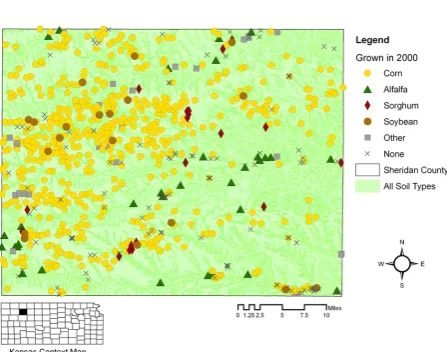
Data on all irrigated land parcels in Kansas are available in a unique database maintained by the Kansas Division of Wa-ter Resources (KDWR). Irrigators in Kansas are required to report their yearly water use by parcel to the KDWR. The an-nual report for each parcel also includes the type of irrigation system, the crop(s) grown, the number of acres irrigated, and the yearly irrigated water volume. These reports are com-piled and distributed via a publicly available GIS data pro-duct, the Water Information Management and Analysis Sys-tem (WIMAS, Fig. 2). Although WIMAS data are spatially comprehensive and detailed, they have some shortcomings.

2_{Estimation of wheat parameters was deferred because the}

ex-tra programming complexity required to split activities across two calendar years was not seen as necessary to evaluate the approach.

Table 1. EPIC parameters to be estimated.

Parameter Description Units

IRI Minimum application interval d for automatic irrigation

BIR Water stress factor to trigger None automatic irrigation –

irrigation occurs on days where the ratio of biomass produced to potential production given adequate water falls below BIR

ARMN Minimum volume allowed mm for automatic irrigation in

a single application

ARMX Maximum volume allowed mm for automatic irrigation in

a single application WA Biomass to energy ratio –

the amount of plant tissue T ha−1MJ−1 (dry weight) produced per

unit of solar energy

TB Optimum temperature ◦C for plant growth

TG Minimum temperature ◦C for plant growth

DLAI Fraction of growing season

completed when the ratio of % leaf area to ground

area (LAI) begins to decline

RLAD Leaf area decline rate – None an index of the rate at which

LAI declines after DLAI

RBMD Biomass-energy decline rate – None an index of the rate at which

WA declines after DLAI

First, several variables needed to identify production rela-tionships (crop yields and the levels of other inputs such as fertilizers and pesticides) are not included. Second, if mul-tiple crops are grown on a given parcel, the irrigator is not required to report the subdivision of acreage or water allo-cation. Third, although points of diversion are increasingly metered, water use reports from un-metered sites may have significant error. These limitations mean that estimation must be robust in the face of uncertain data (see Sect. 4).

Table 2. Parameter ranges used in the estimations.

Parameter Units EPIC Corn Alfalfa Sorghum Soybean

IRI d 1–200 3–14 3–14 3–14 3–14

BIR None 0.2–0.95 0.5–0.95 0.5–0.95 0.5–0.95 0.5–0.95

ARMN mm 1–100 7–14 7–14 7–14 7–14

ARMX mm 10–300 25–45 25–45 25–45 25–45

WA T ha−1MJ−1 10–50 40–60 20–50 10–50 10–40

TB ◦C 10–30 20–35 20–35 20–37 25–35

TG ◦C 0–12 5–15 0–12 0–15 5–15

DLAI % 0.4–0.99 0.75–0.95 0.75–0.95 0.75–0.95 0.75–0.95

RLAD None 0–10 0–10 0–10 0–10 0–10

RBMD None 0–10 0–10 0–10 0–10 0–10

Fig. 2. Well locations in Sheridan Co. KS. Wells are visually coded to show the crop grown in 2000. The most common crop is corn.

County soils were combined into two groups using data from the Soil Survey Geographic (SSURGO, http://soildatamart. nrcs.usda.gov) database maintained by the Natural Resources Conservation Service of the United States Department of Agriculture. Group I contains silt loam soils with slopes be-tween 1 and 3%. This group contains ca. 76% of the land area and 663 of 779 total wells in the county. The second group includes all soils with slopes greater than 5%. This group consists of loam, silt loam and silty clay loam soils and ac-counts for ca. 23% of the land and 93 wells. The remaining ca. 1% of the land and 23 wells were discarded. Thus, each simulation of the crop production associated with a well uti-lizes one of the five sources of weather data and one of the two soil groups. Of the possible 8316 well-years in the si-mulation period (756 wells over 11 years), 4931 of them were used in the calibration. The WIMAS data reported that the other 3385 well-years either did not grow a crop or grew a crop that was not one of the four included in the this study (or multiple crops were grown).

We ensured that each crop was represented by at least one well in each year. Table 3 shows the distribution of all

4931 well-year combinations and the corresponding break-down of total irrigation water usage. Irrigation accounted for 98.8% of all water pumped in Sheridan County during the study period and the well-years in this study totaled 81.3% of all irrigation usage.

Because policy analysis will ultimately entail large amounts of computing power (Steward et al., 2009a), it is desirable to understand the relationship between sample size and estimation outcomes. Thus, a ca. ten percent sub-sample of corn well-years was randomly selected from five clusters identified in each soil group via the Getis and Ord (1992)G∗_i

statistic. The well clusters were based on (1) maximum re-ported volumes of water pumped in any of the 11 years and (2) spatial propinquity (Fig. 3).

4 Maximum entropy estimation

Maximum entropy (ME) (Golan et al., 1996) estimation en-tails maximizing an information theoretic measure of uncer-tainty (entropy,H) subject to constraints imposed by data. The results are probabilistic estimates of parameter values that are as certain as the data allow, but no more so. ME equa-tions remain solvable even in cases where sparse data render the corresponding Least Squares (LS) and Maximum Likeli-hood (ML) equations indeterminate. ME estimation has be-come increasingly popular in many situations, particularly in models where the data are incomplete because the variables of interest are measured at high levels of aggregation. In the field of production economics, several researchers have invoked ME estimation to recover disaggregated production relationships (e.g., crop yield as a function of field-level in-puts) from aggregate data (Howitt and Msangi, 2002; Lence and Miller, 1998; Lansink et al., 2001; Golan et al., 1994, 1996). The parameter values obtained through the estima-tion procedure were not estimated for individual fields, as the values were assumed to be representative across the study re-gion, which is relatively homogeneous in terms of soils, wa-ter availability, farming practices/technology, etc.

Analytically, EPIC can be represented as a mapping from the combined spaces of model inputs and parameters to a space of outputs. More formally, if there are a total ofJ

input variables (soil characteristics, weather conditions, irri-gation amounts, etc.), and all inputs are real numbers, then EPIC inputs can be represented as a vector x∈<J. Simi-larly, if there areKparameters, each of which is known to lie in an interval with finite bounds, then the parameters are a vectorβ∈B, a hypervolume in<K. For simplicity, assume initially that the only model output of interest is crop yield,

y, which is always non-negative. EPIC is then a mapping

Fy : <J×B→<+, and a yield prediction for a given

situa-tion can be written asy=Fy(x;β).

The ME procedure estimates the probability distributions of the unknown parametersβ. Letzkbe anM-dimensional vector of support points along thekth dimension ofB, and let pk be the corresponding vector of probabilities; i.e.,

pmk=Prob[βk=zmk], m=1, . . . , M. For a givenpk, the es-timated value ofβk can be written aszT_kpk, wherezT_k is the transpose ofzk. The simplest specification is where there are two support points for each parameter, corresponding to upper and lower bounds of the known range. In this case, the estimate of thekth parameter isβk=pkz1k+(1−pk)z2k. In the general case, the entire parameter vector can be written compactly as β=Zp, where p=(p1, . . . ,pK) and Z=diag(zT₁, . . . ,zT_K).

If all input data,xij, and yield datayij=Fy(xij;β)were available for each of i=1, . . . , n years and ji=1, . . . , mi wells whereKP

imi, thenβcould be estimated via ME, LS or ML (see Welch et al. (2002) or Steward et al. (2008) for an LS example). However, in the current situation, only

Table 3. Distribution by crop of well-years by soil group and water use.

Crop Soil Group Irrigation I II Water (106m3)

Alfalfa 223 27 19.2

All Corn 3870 374 781.4 10 pct. Corn 521 56 108.9

Sorghum 285 27 30.6

Soybean 116 9 15.0

(a) Maximum water pumped by each well.

(b) Clustered wells. A banded northwest-to-southeast (greater to lesser) trend in pumping is evident.

Fig. 3. Wells in Sheridan Co. KS on a map of Group I (largely silt loam) soils.

the average yields,y_i, for the study area are known, ME still provides an estimate ofβ. One solves

H =max

p>0(

subject to:

y_i = m X

j=1

ωjFy(xij;Zp)

! _m X

j=1

ωj !

(2)

1=pT_k1M, k=1, . . . , K (3) whereH is entropy andωj is the area irrigated by wellj, and 1M is anM-dimensional vector of ones. This is solvable no matter how sparse the yield data because the constraint that probabilities sum to one is, alone, sufficient to determine ap(namely, the uniform distribution wherepmk=(MK)−1). The foundations of entropy estimation are described in detail in Golan et al. (1996). The ability to handle limited data differs drastically from LS and ML where the rank of the governing equations is determined by the number of observa-tions and must at least equal the dimensionality of the vector of unknown parameters.

The description just given readily generalizes to the case of multiple dependent variables (here, crop yield,y (t/ha), and water use,w(mm-ha)) or data statistics (e.g., one might also seek to mimic higher moments of inter-annual water use). Additional information is simply added as further optimiza-tion constraints. This flexibility to tailor the problem state-ment to the information available is another reason for ME’s increasing utilization.

5 Optimization methodology

The genetic algorithm (GA) (Goldberg, 1989), an optimiza-tion procedure based on Darwinian evoluoptimiza-tion, was applied to maximize H. GA possess a number of desirable fea-tures that make them an attractive optimization method for this study. They are quite robust in the presence of local op-tima and both theoretical studies as well as simulations with real-world problems suggest that they are quite effective in obtaining very good solutions. In addition, the vast existing literature on the topic allows one to choose from a variety of operators to suit the needs of a particular optimization prob-lem.

For these reasons, GA have been widely employed in the parameter estimation of models such as EPIC. Zhang et al. (2009) found GA to perform well compared to other opti-mization algorithms in the calibration of the SWAT model. Multi-objective GA have been used in the calibration of this model (Bekele and Nicklow, 2007; Whittaker et al., 2007) as well. GA have also been used to calibrate runoff models such as HBV (Seibert, 2000) and TOPSIS (Cheng et al., 2006) as well as crop (Dai et al., 2009) and crop-related models such as SWAP (He et al., 2007).

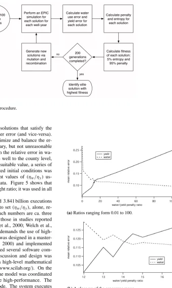
GA operates on a population of trial solutions (100 in this study), each of which is a vector of probabilities, p. The population was initially seeded with random vectors that were normalized to become probabilities summing to unity (Fig. 4). In each of 200 iterations (called generations) per

estimation run, the solutions were updated by means of two operators, mutation and recombination. Mutation was ac-complished by adding a small, random perturbation to each probability in the solution. The sum of all perturbations added to any vector was zero so mutated vectors still summed to one; appropriate limits kept probabilities between zero and one. During recombination, existing pairs of solutions (called parents) were used to create new ones (offspring) ac-cording to

1p0=(λ)1p+(1−λ)2p (4)

2p0=(1−λ)1p+(λ)2p (5)

In the above equation,1pand2pare the two parent vectors

and1p0, 2p0 the offspring. The quantity λ was randomly

distributed in the interval [0, 1].

The selection of parents during crossover was done in a manner motivated by Darwinian survival of the fittest. To obtain each parent, two candidate solutions were drawn ran-domly from the population and the fitter one chosen. The fitness of any solution,p, was

f (p)= −pT lnp−c(p), (6) where the first term is the entropy and c(p) was a func-tion that penalized solufunc-tions which violated any data con-straint. Although not uncommon in mathematical optimiza-tion, penalty functions must be carefully designed. Sub-stantial constraint violations may result when penalties are too mild. Excessively harsh penalties can prevent the com-puter from finding any solution, even when one exists. Additionally, (1) variation in the numerical magnitudes among model outputs will differentially affect the penalty and (2) the investigators may prefer to predict some variables more accurately than others.

To ameliorate differences in numerical magnitudes, the penalty function was defined as the weighted sum of the rel-ative absolute errors

c(p)=λH 

  

Pn i=1

yi−

Pm

j=1ωjFy(xij;Zp)

Pm

j=1ωj

Pn

i=1yi



  

+λH

_η w ηy

Pn i=1

Pm

j=1|wij−ωjFw(xij;Zp)|

Pn i=1

Pm j=1wij

Generate 100 random solutions

Perform an EPIC simulation for each solution for

each well-year

Calculate water use error and yield error for each solution

Calculate penalty and entropy for

each solution

Calculate fitness of each solution: 5% entropy and 95% penalty 200

generations completed?

no

Identify elite solution with highest fitness

yes

Generate new solutions via mutation and recombination

Fig. 4. Overview of the optimization procedure.

variables in opposite directions: solutions that satisfy the yield constraint result in high water error (and vice-versa). For this reason, we sought to minimize and balance the er-ror of both constraints. An arbitrary, but not unreasonable value for(ηw/ηy)is one for which the relative error in wa-ter use, when aggregated from the well to the county level, equals that of yield. To identify a suitable value, a series of 20 estimation runs with randomized initial conditions was performed for each of 14 different values of (ηw/ηy) us-ing the ten percent sample corn data. Figure 5 shows that

(ηw/ηy)=14 is an appropriate weight ratio; it was used in all subsequent runs.

The entire investigation entailed 3.841 billion executions of the EPIC odel; the pilot study to set(ηw/ηy), alone, re-quired 616 million simulations. Such numbers are ca. three orders of magnitude greater than those in studies reported just a few years ago (e.g., Irmak et al., 2000; Welch et al., 2002). Computation of this scale demands the use of high-performance computing. The GA was designed in a master-slave parallel fashion (Cantu-Paz, 2000) and implemented as a scalable system that hybridized several software com-ponents. The interdisciplinary discussion and design was facilitated by writing the GA in a high-level mathematical scripting language (Scilab, http://www.scilab.org/). On the other hand, parallel execution of the model was coordinated by a client written in C to achieve high-performance. The model itself is a legacy Fortran code. The system executes on both dedicated clusters via MPI (Graham et al., 2006) and in a loosely-coupled, distributed fashion via Condor (Thain et al., 2005). The simulations were performed on a 200 CPU Beowulf cluster at Kansas State University and a 200 node Condor pool at the University of Oklahoma. Software perfor-mance measures and scalability were reported in (Bulatewicz et al., 2007).

(a) Ratios ranging form 0.01 to 100.

(b) A close up of the crossover range.

6 Computations and discussion

There are several general questions to ask in a parameter es-timation study of this type. First, what are the resulting esti-mates and what can be said about their uncertainty? Second, how reasonable are the results in terms of both the individual estimates and their interrelationships? Third, ME integrates all sources of information in determining its results, includ-ing both the data as well as the prior information available to the investigators and expressed in the initial ranges set for the parameters. What has been the relative influence of these two factors on the outcome? Fourth, what level of predictability has been achieved?

6.1 Estimates and reasonableness

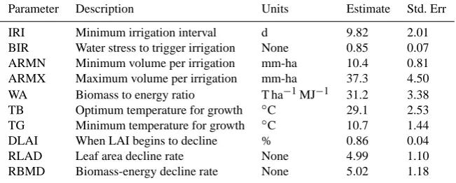
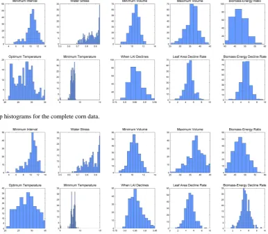
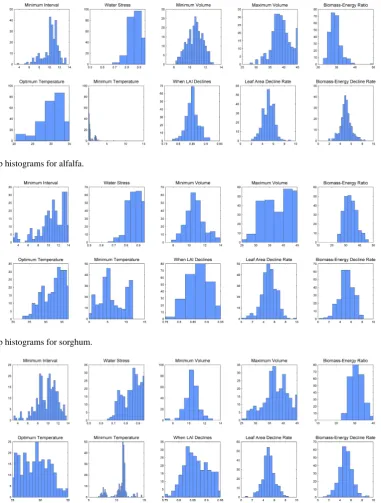
To address these issues in an integrated way, a bootstrap procedure was used (Efron and Tibshirani, 1993). For each of 250 replicates, a random sample of 11 years was selected with replacement from the data and a set of parameter es-timates obtained. On average, each replicate contained ca. seven unique years. To ensure that the variation within the resample structurally reflected that within the original data, the wells in each year were further re-sampled by soil type and weather station. This was done for all crops, including separate runs for the ten percent sample and complete corn data sets. Averaging the best estimates of the 250 replications gives the final estimates (Tables 4 to 7). The standard devia-tions of the 250 estimates are the bootstrap standard errors of the parameters. The shape of the probability distribution for each parameter can be approximately visualized by plotting a histogram of the estimates from the individual bootstrap replications. The histograms indicate the number of times that a parameter value was estimated to be in a given range out of 250 bootstrap replications for each crop (Figs. 6–10).

An immediate result is that the parameter values estimated using the complete corn data were found to closely match the values estimated using only the ten percent sample of corn data. The difference in each estimated value was less than 1% for most parameters, with the largest difference being 5% for the maximum volume per irrigation (ARMX) parameter. Optimization of the three variables that are associated with irrigation system management (IRI, ARMN, and ARMX, Ta-ble 1) resulted in similar values across the four crops (Ta-bles 4 to 7). The minimum application interval (IRI) for all crops was approximately 10.3 d (Tables 4 to 7) and is longer than typically experienced under current production and en-vironmental constraints. Given sufficient data, EPIC applies reasonable total amounts of water on a countywide basis (e.g. corn in Table 8), but appears to do so in fewer, larger, appli-cations. The average well capacity for all wells 45 ha. Us-ing these values, it is possible to apply an irrigation depth of 37 mm every 5.4 d. A common practice is for constant irri-gation during critical growth stages so as to maximize yields. Additional model runs indicate that EPIC outputs are not

par-ticularly sensitive to IRI in the range of 4 to 10 d, but sensi-tivity increases above this point (data not shown). A shal-low minimum in f (p)slightly above 10 d could therefore account for our results. To the best of our knowledge, no prior studies have calibrated IRI so this model feature has not previously been detected. It is potentially important in that it suggests that irrigation scheduling could possibly reduce water use while maintaining yields. The minimum and max-imum volumes for automatic irrigation (ARMN and ARMX, respectively) resulted in mean values across all four crops of 10.6 and 37.6 mm per application, respectively. While real-istic in terms of typical irrigation practices, these limits are broad enough to encompass a model shift from more numer-ous smaller applications to fewer, larger ones.

The physiologically-based variables followed trends pre-viously reported from field and greenhouse experiments as well as other crop modeling efforts. The water stress level to trigger irrigation (BIR) is specified in terms of biomass pro-duction: irrigation occurs on days where the ratio of biomass produced to potential production (given adequate water) falls below BIR. The BIR values for corn, grain sorghum, alfalfa, and soybean are 0.86, 0.87, 0.87, and 0.85, respectively – not unreasonable for irrigated cropping conditions where water stress is less likely to occur.

Optimized parameters that not unexpectedly had species-specific ranges are biomass to energy conversion ratio (WA), optimum temperature for growth (TB), and minimum tem-perature of growth (TG). Optimized values for WA were 47.0 for corn (complete data), 33.4 for grain sorghum, 29.2 for al-falfa, and 31.2 for soybean. Reported corn WA values ranged from 14.5 to 43.3 t ha−1_MJ−1_m−2 _{(Cantarero et al., 1999;}

Muchow, 1990; Hammer et al., 1998; Kiniry et al., 2004; Idi-noba et al., 2002; Sinclair and Muchow, 1999) with the range being attributed to differences in environmental conditions and calculation method. Reported WA specifically for use in crop models for corn have ranged from 43.3 in CERES-Maize (Yang et al., 2004), 39.8 for ALMANAC (Kiniry et al., 2004) and 35.0 to 40.0 t ha−1MJ−1m−2 for CropSyst (Stockle et al., 2003).

For grain sorghum, reported WA values have ranged from 16.0 to 28.0 t ha−1MJ−1m−2(Muchow, 1989; Sinclair and Muchow, 1999). However, values used in sorghum crop models range from 32.0 in SORKAM (Rosenthal et al., 1989) to 35.0 to 40.0 t ha−1MJ−1m−2in CropSyst (Stockle et al., 2003), which are very similar to those found here.

Table 4. Parameter estimates for corn.

Parameter Description Units All Data/10 pct. Sample Estimate Std. Err

IRI Minimum irrigation interval d 10.3/10.3 1.52/1.58 BIR Water stress to trigger irrigation None 0.86/0.85 0.07/0.08 ARMN Minimum volume per irrigation mm 10.5/10.4 0.75/0.87 ARMX Maximum volume per irrigation mm 35.9/37.6 2.99/3.87 WA Biomass to energy ratio T ha−1MJ−1 47.0/47.6 3.32/3.41 TB Optimum temperature for growth ◦C 27.2/28.1 3.38/3.47 TG Minimum temperature for growth ◦C 8.20/8.23 0.52/0.62 DLAI When LAI begins to decline % 0.86/0.86 0.03/0.03 RLAD Leaf area decline rate None 4.95/5.03 1.03/1.14 RBMD Biomass-energy decline rate None 5.17/5.14 1.11/1.10

Table 5. Parameter estimates for alfalfa.

Parameter Description Units Estimate Std. Err

IRI Minimum irrigation interval d 10.3 1.56 BIR Water stress to trigger irrigation None 0.87 0.05 ARMN Minimum volume per irrigation mm-ha 10.7 0.99 ARMX Maximum volume per irrigation mm-ha 39.1 3.34 WA Biomass to energy ratio T ha−1MJ−1 29.2 3.04 TB Optimum temperature for growth ◦C 30.4 3.06 TG Minimum temperature for growth ◦C 0.50 0.81 DLAI When LAI begins to decline % 0.85 0.02 RLAD Leaf area decline rate None 5.08 1.03 RBMD Biomass-energy decline rate None 5.01 0.98

Table 6. Parameter estimates for sorghum.

Parameter Description Units Estimate Std. Err

IRI Minimum irrigation interval d 10.8 2.59 BIR Water stress to trigger irrigation None 0.87 0.06 ARMN Minimum volume per irrigation mm-ha 10.8 1.14 ARMX Maximum volume per irrigation mm-ha 38.3 5.13 WA Biomass to energy ratio T ha−1MJ−1 33.4 4.39 TB Optimum temperature for growth ◦C 32.5 3.35 TG Minimum temperature for growth ◦C 6.19 3.36 DLAI When LAI begins to decline % 0.87 0.04 RLAD Leaf area decline rate None 4.99 1.39 RBMD Biomass-energy decline rate None 5.10 1.26

Table 7. Parameter estimates for soybean.

Parameter Description Units Estimate Std. Err

Table 8. Relative errors.

Crop Yield Water

Means Bootstrap Replicates Means Bootstrap Replicates

Fitted Fitted Predictive Fitted Fitted Fitted Predictive County County County County Well County Well County Well

10 pct. Corn 0.09 0.11 0.14 0.16 0.32 0.15 0.31 0.21 0.35

90 pct. Corn 0.09 a a 0.13 0.33 a a a a

All Corn 0.09 0.10 0.13 0.13 0.32 0.13 0.32 0.19 0.35 Alfalfa 0.16 0.17 0.20 0.21 0.43 0.22 0.43 0.27 0.46 Sorghum 0.10 0.10 0.13 0.25 0.46 0.24 0.44 0.31 0.49 Soybean 0.18 0.20 0.25 0.31 0.42 0.25 0.38 0.34 0.45

All Crops 0.09 b b 0.13 c d d d d

a_{Not separately bootstrapped.}b_{Different grains are not commensurate.}c_{Single wells are single crops.}d_{Analysis would require averaging}

(number of bootstrap reps)(number of crops)scenarios (ca. 3.9×109).

Fig. 6. Bootstrap histograms for the complete corn data.

Fig. 7. Bootstrap histograms for the ten percent corn data.

Soybean WA values from field experiments have been reported to be 20.0 (Sinclair and Muchow, 1999). CropSyst initial WA values are reported as 20.0 to 25.0 t ha−1MJ−1m−2 which is lower than the WA of 31.2 that resulted from the optimization process we used. The po-tential radiation use efficiency (WA) in EPIC is assumed to

Fig. 8. Bootstrap histograms for alfalfa.

Fig. 9. Bootstrap histograms for sorghum.

Fig. 10. Bootstrap histograms for soybean.

The estimated optimum temperatures for growth (TB) were 27.2◦_{C for corn (complete data), 32.5}◦_{C for grain}

sorghum, 30.4◦_{C for alfalfa and 29.1}◦_{C for soybean. Several}

researchers have reported optimum temperatures for growth in corn to be 22.5◦C (Wilhelm et al., 1999) and 25◦C (Grze-siak et al., 1981). CERES-Maize uses 26◦C as the optimum temperature for growth (Jones et al., 1986) while Yang et al. (2004) currently use 30◦C in the Hybrid Maize model for maximum growth and assimilation. Our optimized corn

temperature for optimum growth is within the range of the values used by other simulation models and slightly higher than those reported from research trials. Our estimated TB for grain sorghum (32.5◦_{C ) agrees with the results of Prasad}

The TB estimate of 30.4◦_{C for alfalfa is higher than the}

reported values of 20 to 27◦_{C cited by several others (Arbi}

et al., 1979; Fick, 1984; Bula, 1972; Ueno and Smith, 1970; Pearson and Hunt, 1972). However, our TB value is simi-lar to the 30◦C used by Confalonieri and Bechini (2004) in their optimization of CropSyst. Our estimate of 29.1◦C for soybean is higher than the 24 to 27.5◦C reported by Sed-digh and Jolliff (1984) and Ghazali and Cox (1981), but is in agreement with Gibson and Mullen (1996) and Grimm et al. (1994) who reported optimum temperatures for photosyn-thesis and growth to range from 29 to 35◦C. Our TB is less than that used in CROPGRO-Soybean, which uses 40◦C as an optimum temperature for photosynthesis (Pedersen et al., 2004).

The estimated minimum temperatures for growth (TG) were 8.2◦_{C for corn (complete data), 6.2}◦_{C for grain}

sorghum, 0.5◦C for alfalfa, and 10.7◦C for soybean. These estimates are similar to those reported by others from field or growth chamber research or currently being used in other crop simulation models. Reported corn TG values range from 7.2 to 8◦C (Hesketh and Warrington, 1989; Yang et al., 2004). For grain sorghum, a TG of 8.5◦C is reported by both Craufurd et al. (1998) and Hammer et al. (1989) while SORKAM (Rosenthal et al., 1989) uses 7◦C as a base tem-perature, all of which are marginally higher than the 6.2◦C estimated here.

Estimates of TG for alfalfa of 0.5◦_{C are lower than the}

5◦_{C used by Confalonieri and Bechini (2004) in calibrating}

CropSyst for simulating alfalfa in Italy. Our TG of 10.7◦C for soybean is greater than that used in CROPGRO-Soybean, which uses 8◦C as base temperature for photosynthesis (Ped-ersen et al., 2004).

Estimates of when leaf area begins to decline (DLAI), the rate of decline (RLAD) and the rate at which WA declines (RBMD) could be deemed reasonable based on typical pro-duction scenarios. For all four crops, the values for DLAI indicate that leaf area begins to decline after around 86% of the growing season has occurred. Leaf area typically begins a gradual decline in corn and grain sorghum within approxi-mately 1 week of anthesis, but this largely occurs in the lower canopy and the loss represents older leaves that will not con-tribute to final yields. However, more rapid leaf loss near physiological maturity typically happens in all three grain crops and appears to be captured appropriately in our results for these three variables. In alfalfa, it is difficult to determine how these values compare to reality since this perennial crop does not normally senesce as it is typically harvested at 10% bloom stage. The final harvest timing recommendation is af-ter cold temperatures induce dormancy in the crop.

6.2 Influence of prior information

Maximum entropy estimation makes use of the complete cor-pus of available information. Thus, the standard errors re-ported in Tables 4 to 7 reflect notonly the data but also the

prior information implicit in the selected probability sup-port points. As just documented, the optimizations resup-ported herein did produce reasonable output values. Even so, it is possible that the data do not constrain the estimates either because (1) they are too fragmentary or (2) the parameter’s influence on actual outcomes is too weak or indirect. It is therefore useful to ask (Q1) do the data detectably influence the outputs and (Q2) how strongly does prior information af-fect the estimates?

If a parameter has no influence on the model outputs then it cannot affect the penalty function values. In this situation

f (p)is optimized when H is maximized. In a two-point distribution this happens when the parameter estimate is the midpoint of the support interval no matter where the end-points are located. Based on this fact, metrics for Q1 and Q2 were developed and applied to the ten percent corn sam-ple. The Q1 metric calculates a two-tailed, binomial distri-bution p-value for the null hypothesis that the median of the 250 re-sampled parameter estimates is the midpoint of the support range. A p-value of less than 0.05 is interpreted as a significant data influence. The easiest way to measure de-pendence on the support point choice is to make a different choice. Thus, the Q2 metric is a finite difference estimate of the derivative of the parameter estimate with respect to the midpoint of the parameter range. Values close to unity are consistent with the estimate being completely dependent on prior information. Ten sets of 20 estimations were run with the range of a single parameter changed in each set. The ranges were shifted up or down depending on whether the majority of the original estimates did or did not exceed the midpoint. Range widths were preserved unless doing so re-sulted in an endpoint that was (1) outside the range suggested by EPIC, or (2) conflicted with the range of another parame-ter.

The results are in Table 9. All but three parameters (DLAI, RLAD and RBMD) are influenced by the data with more significant median departures from the support interval mid-points being generally associated with lower sensitivities to prior information. It is clear, however, that the Q1 and Q2 metrics measure different properties of the estimation pro-cess, as illustrated by ARMN which responds both to prior information and to data. TG shows a similar pattern but with a lower dependence on prior information. The unit sensitivity to prior information displayed by RLAD and RBMD coupled with their close adherence to the support interval midpoint, suggests that these parameters are poorly constrained by the data.

6.3 Model verification

Table 9. Analysis of the influence of prior information on corn parameters.

Parameter Units Ranges Estimates Metrics

Initial Alternate Initial Alternate Q1 Q2

IRI d 3–14 8.5–19.5 10.3 11.5 <10−5 0.22

BIR None 0.5–0.95 0.725–0.95 0.85 0.89 <10−5 0.38

ARMN mm 7–14 3.5–10.5 10.4 6.89 0.0497 1.00

ARMX mm 25–45 35–55 37.6 43.2 <10−5 0.56

WA T ha−1MJ−1 40–60 30–50 47.6 45.0 <10−5 0.25

TB ◦C 20–35 15–27.5 28.1 23.5 0.0191 0.74

TG ◦C 5–15 0–10 8.23 5.86 <10−5 0.47

DLAI % 0.75–0.95 0.65–0.85 0.86 0.81 0.3428 0.52

RLAD None 0–10 0–5 5.03 2.61 0.9496 0.97

RBMD None 0–10 0–5 5.14 2.55 0.2294 1.04

well they could predict the years that had been omitted in each replicate (“Fitted” and “Predictive”, respectively, in Ta-ble 8). Depending on the crop, the variaTa-ble (yield or wa-ter use) and, for wawa-ter, the level of aggregation (county- vs. well-level) attempting to predict independent, out-year data increased the error from 3 to 9% of full scale. The predic-tive water use errors were quite high at the well level ranging from 35% for the complete and ten percent corn sample to 49% for sorghum. However, for aquifer modeling, accuracy at this fine a geographic scale may not be needed. Predictive errors at the county level were smaller.

Second, we used the mean parameter estimates obtained from the ten percent corn sample to estimate the behavior of the remaining 90% of the data. The performance was es-sentially identical, confirming the ability of a small sample to enable accurate estimation of a much larger set from the same years. The selection procedure for the ten percent sam-ple was designed to achieve good representation. There are two ways this could have failed: the estimates might have deviated from those of the larger sample or the full data set might have had much greater variability. The latter would have resulted in larger relative errors even if the mean predic-tions were accurate. Clearly neither of these happened. How-ever, the bootstrap relative errors show that the inter-annual variability is such that samples of 7 out of 11 years can only capture it to the degree shown in the Predictive columns, at least at the single county scale. Of course, incorporating data from more than one county may serve to offset temporal vari-ation. Finally, the relative error in total county irrigation use for these four crops is 13%, which is the same as that for corn, due to its heavy preponderance in the county.

Third, the county-level yield and water use errors are within 5% of each other in all cases but sorghum, in which the error difference was 14%. This suggests that a penalty ratio of 14 was effective in balancing thecounty-level yield and water use error, but that crop-specific penalty ratios may give better results.

Table 10. Standard errors.

Crop

RMSE RMSEP

Yield Water Yield Water (t/ha) (mm-ha) (t/ha) (mm-ha)

10 pct. Corn 1.58 69.7 1.85 93.4 All Corn 1.44 59.8 1.71 82.5 Alfalfa 2.11 78.2 2.38 90.9 Sorghum 0.88 78.3 1.06 99.6 Soybean 0.83 102.8 0.93 130.1

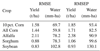
Finally, whereas relative errors are dimensionless frac-tions, Table 10 reports county-level yield and water use er-rors in physical units. The two left columns are the root mean square errors (RMSE) resulting from running simulations us-ing each of the 250 estimates against the complete data. The two right columns are the root mean square errors of predic-tion (RMSEP) and are calculated in the same way except that the 250 estimates were used to predict the years that had been omitted in each replicate. These latter numbers may be taken as an indication of expected model performance using data collected from a single county. These RMSE of water use and the well-level relative error (Table 8) both reflect the ac-curacy of the simulations at the field scale. When aggregated to the county scale, there is a significant reduction in the er-ror (compare well- and county-level relative erer-ror of water use in Table 8).

7 Conclusions

the integration of a range of methodologies whose cross-disciplinary fusion enables a much broader range of acti-vities. This integration reaches across diverse disciplines: agronomy, agricultural economics, civil engineering, com-puter science, and electrical engineering. The specific tech-nologies are correspondingly diverse: crop physiological simulation, maximum entropy estimation, genetic algorithm-based optimization, alternative parallel processing method-ologies, GIS databases, and cluster analysis, to name a few.

Through the integration of these technologies, a genetic algorithm that employed ME was able to identify realistic values for ten crop model parameters including both hydro-logical and physiohydro-logical inputs. The estimated parameter values were not only realistic, but they were able to repro-duce observed irrigation water use to within 13% with an estimated predictive accuracy of 19% (complete corn data) given sufficient data. In addition, several of these parameters represent irrigation practice, effectively recovering detailed irrigator behavior from annual water use reports. Knowl-edge of this kind is otherwise unavailable yet is essential for the prediction of water use in alternative scenarios as part of an investigation into effective water policy for sustain-able usage. Such a policy analysis would entail consider-able computational requirements. These demands could be mitigated through the use of carefully selected samples of data with only slight increases in error, as demonstrated in this work through the evaluation of the ten percent sample of corn data. The implementation of these techniques has provided a framework within which additional models and data will be integrated. The particular team assembled for this paper crosses the spectrum of hydrologists, agronomists, economists, and computer scientists, and the results are be-ing shared and translated by disciplinary specialists to inte-rested collaborators, stakeholders and agencies with which the team is working. Examples include applications of the calibrated model in both irrigation studies and in the assess-ment of the economic impacts of water policy on farmers in western Kansas as part of an integrated model.

Bordogna (2003) wrote: “The trick in evolving the capa-bility for providing emergent infrastructure is the selective use of established models and the rapid generation and test-ing of new models. This is a process of institutional and or-ganizational learning, and the ability to learn rapidly is itself a kind of social infrastructure that is required to pursue the cyberinfrastructure vision.” We believe that studies such as this one are important steps along that learning path.

Acknowledgements. This work was supported in part by the National Science Foundation (Projects EPS0553722, EIA0092839, #020313 and CCR-0082667), USDA/ARS (Cooperative Agree-ment 58-6209-3-018), the Kansas State University Provost’s Office Targeted Excellence Program, and Hatch Project 0311 through the Kansas Agricultural Experiment Station. Any findings, opinions, conclusions, or recommendations expressed herein are those of the authors and do not necessarily reflect the views of

any funding units. Assistance in using computing facilities at the University of Oklahoma was graciously provided by the Oklahoma Supercomputing Center for Education and Research. Guidance in the production of the figures included in this work was provided by E. A. Bernard, Landscape Architecture, Kansas State University.

Edited by: N. Verhoest

References

Aigner, D. J. and Goldfeld, S. M.: Estimation and prediction from aggregate data when aggregates are measured more accurately than their components, Econometrica, 42, 113–134, 1974. Arbi, N., Smith, D., and Bingham, E. T.: Dry matter and

morpho-logical responses to temperatures of alfalfa strains with differing ploidy levels, Agron. J., 71, 573–577, 1979.

Bekele, E. G. and Nicklow, J. W.: Multi-objective automatic cali-bration of SWAT using NSGA-II, J. Hydrol., 341(3–4), 165–176, 2007.

Berck, P. and Helfand, G.: Reconciling the von Liebig and differen-tiable crop production functions, Am. J. Agr. Econ., 72(4), 985– 996, 1990.

Bernard, E. A., Peterson, J. M., and Steward, D. R.: A cou-pled hydrologic-economic modeling tool to support groundwa-ter management decisions, in: Proceedings of the 2004 High Plains Groundwater Resources: Challenges and Opportunities, Lubbock, Texas, p. 82, 7–9 December 2004.

Bernard, E. A., Steward, D. R., and Le Grand, P.: A geodatabase for groundwater modeling in mlaem and modflow, in: Proceed-ings of the 2005 ESRI International User Conference, San Diego, California, Paper number 1633, 1–25, 25–29 July 2005. Bernardos, J. N., Viglizzo, E. F., Jouvet, V., Lertora, F. A.,

Por-domingo, A. J., and Cid, F. D.: The use of epic model to study the agroecological change during 93 years of farming transformation in the argentine pampas, Agr. Syst., 69(3), 215–234, 2001. Bordogna, J.: US engineering: Enabling the nation’s capacity to

perform, The Bent of Tau Beta Pi, 114(4), 28–32, 2003. Bouman, B. A. M., van Keulen, H., van Laar, H. H., and

Rab-binge, R.: The “school of de wit” crop growth simulation models: A pedigree and historical overview, Agr. Syst., 52(2–3), 171– 198, 1996.

Bowen, W.: Modeling plant and soil systems, in: Agronomy mono-graph no. 31, edited by: Hanks, R. J., and Ritchie, J. T., Agron-omy Society of America, Crop Science Society of America, and Soil Science Society of America, Agr. Syst., 41(4), 526–527, 1993.

Bryant, K. J., Benson, V. W., Kiniry, J. R., Williams, J. R., and Lacewell, R. D.: Simulating corn yield response to irrigation timings: Validation of the epic model, J. Prod. Agric., 5(2), 237– 242, 1992.

Brown, R. A., Rosenberg, N. J., Hays, C. J., Easterling, W. E., and Mearns, L. O.: Potential production and environmental effects of switchgrass and traditional crops under current and greenhouse-altered climate in the central united states: A simulation study, Agr. Ecosyst. Environ., 78(1), 31–47, 2000.

united states growing regions, Climatic Change, 41(1), 73–107, 1999.

Bula, R. J.: Morphological characteristics of alfalfa plants grown at several temperatures, Crop Sci., 12, 683–686, 1972.

Bulatewicz, T., Andresen, D., Welch, S. M., Jin, W., Das, S., and Miller, M.: A software system for scalable parameter estimation on clusters, in: Proceedings of the 8th LCI International Con-ference on High-Performance Clustered Computing, South Lake Tahoe, California, p. 7, 14–17 May 2007.

Cabelguenne, M., Jones, C. A., and Williams, J. R.: Strategies for limited irrigations of maize in southwestern france – a modeling approach, Transactions of the American Society of Agriciultural Engineers, 38(2), 507–511, 1995.

Cantarero, M. G., Cirilo, A. G., and Andrade, F. H.: Night tem-perature at silking affects kernel set in maize, Crop Sci., 39(3), 703–710, 1999.

Cantu-Paz, E.: Efficient and accurate parallel genetic algorithms, Kluwer Academic Publishers, Norwell, MA, USA, 2000. Cheng, C. T., Zhao, M. Y., Chau, K. W., and Wu, X. Y.: Using

ge-netic algorithm and topsis for xinanjiang model calibration with a single procedure, J. Hydrol., 316(1–4), 129–140, 2006. Chowdhury, S. I. and Wardlaw, I. F.: The effect of temperature on

kernel development in cereals, Aust. J. Agr. Res., 29(2), 205– 223, 1978.

Cole, C. V., Williams, J., Shaffer, M., and Hanson, J.: Nutrient and organic matter dynamics as components of agricultural produc-tion systems models, Soil Sci. Soc. Am. Special Publicaproduc-tion, 19, 147–166, 1987.

Collino, D. J., Dardanelli, J. L., De Luca, M. J., and Racca, R. W.: Temperature and water availability effects on radiation and water use efficiencies in alfalfa, Aust. J. Exp. Agr., 45(4), 383–390, 2005.

Confalonieri, R. and Bechini, L.: A preliminary evaluation of the simulation model cropsyst for alfalfa, Eur. J. Agron, 21(2), 223– 237, 2004.

Craufurd, P. Q., Qi, A., Ellis, R. H., Summerfield, R. J., Roberts, E. H., and Mahalakshmi, V.: Effect of temperature on time to panicle initiation and leaf appearance in sorghum, Crop Sci., 38, 942–947, 1998.

Dai, C., Yao, M., Xie, Z., Chen, C., and Liu, J.: Parameter op-timization for growth model of greenhouse crop using genetic algorithms, Appl. Soft Comput., 9(1), 13–19, 2009.

Dautrebande, S., Dewez, A., Casse, C., and Hennebert, P.: Ni-trate leaching at regional scale with epic: an implicit example of a hydrotope model concept, in: International Workshop of Eur. Ag. Engineeering Field of Interest on Soil and Water, Mod-elling of transport processes in soils at various scales in time and space, edited by: Feyen, J. and Wiyo, K., Leuven, Belgium, 765– 774, 24–26 November 1999.

Easterling III, W. E., Crosson, P. R., Rosenberg, N. J., McKen-ney, M. S., Katz, L. A., and Lemon, K. M.: Agricultural impacts of responses to climate change in the missouri-iowa-nebraska-kansas (mink) region, Climatic Change, 24(1–2), 23–61, 1993. Efron, B. and Tibshirani, R. J.: An introduction to the bootstrap,

Chapman and Hall/CRC, Boca Raton, FL, 1993.

Ellis, J. R., Lacewell, R. D., Moore, J., and Richardson, J. W.: Pre-ferred irrigation strategies in light of declining government sup-port, J. Prod. Agric., 6, 112–118, 1993.

Engel, T., Hoogenboom, G., Jones, J. W., and Wilkens, P. W.:

Aegis/win: a computer program for the application of crop sim-ulation models across geographic areas, Agron. J., 89, 919–928, 1997.

Evers, A. J. M., Elliott, R. L., and Stevens, E. W.: Integrated deci-sion making for reservoir, irrigation, and crop management, Agr. Syst., 58(4), 529–554, 1998.

Fick, G. W.: Simple simulation models for yield prediction applied to alfalfa in the northeast, Agron. J., 76, 235–239, 1984. Fortin, M. C. and Moon, D. E.: Errors associated with the use of

soil survey data for estimating plant-available water at a regional scale, Agron. J., 91(6), 984–990, 2000.

Frank, M. D., Beattie, B. R., and Embleton, M. E.: A comparison of alternative crop response models, Am. J. Agr. Econ., 72, 597– 603, 1990.

Geleta, S., Sabbagh, G. J., Stone, J. F., Elliott, R. L., Mapp, H. P., Bernardo, D. J., and Watkins, K. B.: Importance of soil and crop-ping systems in the development of regional water quality poli-cies, J. Environ. Qual., 23(1), 36–42, 1994.

Getis, A. and Ord, J. K.: The analysis of spatial association by use of distance statistics, Geogr. Anal., 24, 189–206, 1992.

Ghazali, N. J. and Cox, F. R.: Effect of temperature on soybean growth and manganese accumulation, Agron. J., 73, 363–367, 1981.

Gibson, L. R. and Mullen, R. E.: Influence of day and night tem-perature on soybean seed yield, Crop Sci., 36, 98–104, 1996. Golan, A., Judge, G., and Robinson, S.: Recovering information

from incomplete or partial multisectoral economic data, Rev. Econ. Stat., 76(3), 541–549, 1994.

Golan, A., Judge, G., and Perloff, J.: Estimating the size distribu-tion of firms using government summary statistics, J. Ind. Econ., 44(1), 69–80, 1996.

Goldberg, D. E.: Genetic algorithms in search, optimization, and machine learning. Addison Wesley, Reading, MA, 1989. Graham, R. L., Shipman, G. M., Barrett, B. W., Castain, R. H.,

Bosilca, G., and Lumsdaine, A.: Open mpi: A high-performance, heterogeneous mpi, in: Proceedings of the Fifth International Workshop on Algorithms, Models and Tools for Parallel Com-puting on Heterogeneous Networks, Barcelona, Spain, 25–28 September, 2006.

Grimm, S. S., Jones, J. W., Boote, K. J., and Herzog, D. C.: Model-ing the occurrence of reproductive stages after flowerModel-ing for four soybean cultivars, Agron. J., 86, 31–38, 1994.

Grunefeld, Y. and Griliches, Z.: Is aggregation necessarily bad?, Rev. Econ. Stat., 42, 1–13, 1960.

Grzesiak, S., Rood, S. B., Freyman, S., and Major, D. J.: Growth of corn seedlings: effects of night temperature under optimum soil moisture or under drought conditions, Can. J. Plant Sci., 61, 871–877, 1981.

Guerra, L. C., Hoogenboom, G., Hook, J. E., Thomas, D. L., Bo-ken, V. K., and Harrison, K. A.: Evaluation of on-farm irriga-tion applicairriga-tions using the simulairriga-tion model epic, Irrigairriga-tion Sci., 23(4), 171–181, 2005.

Hammer, G. L., Vanderlip, R. L., Gibson, G., Wade, L. J., Hen-zell, R. G., Younger, D. R., Warren, J., and Dale, A. B.: Genotype-by-environment interaction in grain sorghum ii effects of temperature and photoperiod on ontogeny, Crop Sci., 29, 376– 384, 1989.

(zea mays), Aust. J. Agr. Res., 49(2), 249–262, 1998.

He, K., Zheng, L., Dong, S., Tang, L., Wu, J., and Zheng, C.: PGO: a parallel computing platform for global optimization based on Genetic Algorithm, Comput. Geosci., 33(3), 357–366, 2007. Hesketh, J. D. and Warrington, I. J.: Corn growth response to

tem-perature: rate and duration of leaf emergence, Agron. J., 81(4), 696–701, 1989.

Howitt, R. E. and Msangi, S.: Reconstructing disaggregate produc-tion funcproduc-tions, in: Proceedings of the Xth Congress of the Euro-pean Association of Agricultural Economists, Zaragoza, Spain, 28–31 August, 2002.

Idinoba, M. E., Idinoba, P. A., and Gbadegesin, A. S.: Radia-tion intercepRadia-tion and its efficiency for dry matter producRadia-tion in three crop species in the transitional humid zone of nigeria, Agronomie, 22, 273–281, 2002.

Irmak, A., Jones, J. W., Mavromatis, T., Welch, S. M., Boote, K. J., and Wilkerson, G. G.: Evaluating methods for simulating soy-bean cultivar responses using cross validation, Agron. J., 92, 1140–1149, 2000.

Jones, C. A., Kiniry, J. R., and Dyke, P. T.: CERES-Maize: A sim-ulation model of maize growth and development, Texas A&M Univ. Press, College Stn., TX, 1986.

Kiniry, J. R., Bean, B., Xie, Y., and P. Chen: Maize yield potential: Critical processes and simulation modeling in a high yielding en-vironment, Agr. Syst., 82(1), 45–56, 2004.

Lal, H., Hoogenboom, G., Calixte, J. P., Jones, J. W., and Bein-roth, F. H.: Using crop simulation models and gis for regional productivity analysis, Transactions of the American Society of Agriciultural Engineers, 36(1), 175–184, 1993.

Lansink, A. O., Silva, E., and Stefanou, S.: Inter-firm and intra-firm efficiency measures, J. Prod. Anal., 15, 185–199, 2001. Lence, S. H. and Miller, D. J.: Recovering output-specific

in-puts from aggregate input data: A generalized cross-entropy ap-proach, Am. J. Agr. Econ., 80(4), 852–867, 1998.

Montaigne, F.: Water pressure, National Geographic, 2–33, September 2002.

Muchow, R. C.: Comparative productivity of maize, sorghum and pearl millet in a semi-arid tropical environment, Field Crop. Res., 20(3), 191–219, 1989.

Muchow, R. C.: Effect of high temperature on grain growth in field-grown maize, Field Crop. Res., 23(2), 145–158, 1990.

Paris, Q.: The von liebig hypothesis, Am. J. Agr. Econ., 74, 1019– 1028, 1992.

Pearson, C. J. and Hunt, L. A.: Effects of temperature of primary growth of alfalfa, Can. J. Plant Sci., 52, 1007–1015, 1972. Pedersen, P., Boote, K. J., Jones, J. W., and Lauer, J. G.: Modifying

the cropgro-soybean model to improve predictions for the upper midwest, Agron. J., 96, 556–564, 2004.

Pesaran, M. H., Peirse, R. G., and Kumar, M. S.: Econometric anal-ysis of aggregation in the context of linear prediction models, Econometrica, 57(4), 861–888, 1989.

Peterson, J. M. and Steward, D. R.: Groundwater economics: object oriented, integrated studies using the aem, in: Proceedings of the 5th International Conference on the Analytic Element Method, Manhattan, Kansas, 26–31, 14–17 May 2006.

Prasad, P. V. V., Boote, K. J., and Allen, L. H.: Adverse high tem-perature effects on pollen viability, seed-set, seed yield and har-vest index of grain-sorghum are more severe at elevated carbon dioxide due to higher tissue temperatures, Agr. Forest Meteorol.,

139(3–4), 237–251, 2006.

Rosenthal, W. D., Vanderlip, R. L., Jackson, B. S., and Arkin, G. F.: Sorkam: A grain sorghum growth model, TAES Computer Soft-ware Documentation Number MP-1669, Texas Agr. Exp. Stn., College Station, Texas, 1989.

Sasaki, K.: An empirical analysis of linear aggregation problems: The case of investment behavior in japanese firms, J. Economet-rics, 7(3), 313–331, 1978.

Seddigh, M. and Jolliff, G. D.: Effects of night temperature on dry matter partitioning and seed growth of indeterminate field-grown soybean, Crop Sci., 24, 704–710, 1984.

Seibert, J.: Multi-criteria calibration of a conceptual runoff model using a genetic algorithm, Hydrol. Earth Syst. Sci., 4, 215–224, 2000,

http://www.hydrol-earth-syst-sci.net/4/215/2000/.

Sharpley, A. N. and Williams, J. R.: Epic – erosion/productivity im-pact calculator: 1 model documentation, USDA Technical Bul-letin, No. 1768, 1990.

Sinclair, T. R. and Muchow, R. C.: Radiation use efficiency, Adv. Agron, 65, 215–265, 1999.

Steward, D. R. and Bernard, E. A., Integrated engineering and land-scape architecture approaches to address groundwater declines in the High Plains Aquifer, Chapter 9 of Case studies in water re-sources, 121–134, edited by: Bhandari, A. and Butkus, M. A., Association of Environmental Engineering & Science Profes-sors, 2006a.

Steward, D. R. and Bernard, E. A.: The synergistic powers of aem and gis geodatabase models in water resources studies, Ground Water, 44(1), 56–61, 2006b.

Steward, D. R., Le Grand, P., and Bernard, E. A.: The analytic ele-ment method and supporting gis geodatabase model, in: Bound-ary Elements 27: Proc. 27th World Conference on BEM/MRM, Orlando, Florida, 187–196, 15–17 March 2005.

Steward, D. R.,Le Grand, P., Jankovic, I., and Strack, O. D. L.: Cauchy integrals for boundary segments with curvilinear geom-etry, Proc. R. Soc. Lon. Ser.-A., 464, 223–248, 2008.

Steward, D. R., Peterson, J. M., Yang, X., Bulatewicz, T., Herrera-Rodriguez, M., Mao, D., and Hendricks, N.: Groundwater eco-nomics: An object-oriented foundation for integrated studies of irrigated agricultural systems, Water Resour. Res., 45, W05430, doi: 10.1029/2008WR007149, 2009a.

Steward, D. R., Yang, X., and Chacon, S.: Groundwater response to changing water-use practices in sloping aquifers using convo-lution of transient response functions, Water Resour. Res., 45, 1–13, 2009b.

Stockle, C. O., Donatelli, M., and Nelson, R.: Cropsyst, a cropping systems simulation model, Eur. J. Agron., 18(3), 289–307, 2003. Thain, D., Tannenbaum, T., and Livny, M.: Distributed computing in practice: the condor experience, Concurrency and Computa-tion: Practice and Experience, 17(2–4), 323–356, 2005. Theil, H.: Linear aggregation of economic relations, North Holland,

Amsterdam, 1954.

Ueno, M. and Smith, D.: Influence of temperature on seedling growth and carbohydrate composition of three alfalfa cultivars, Agron. J., 62, 764–767, 1970.

45, 1163–1175, 2002.

Whitfield, D. M., Wright, G. C., Gyles, O. A., and Taylor, A. J.: Ef-fects of stage growth, irrigation frequency and gypsum treatment of CO2assimilation of lucerne (medicago sativa l.) grown on a heavy clay soil, Irrigation Sci., 7(3), 169–181, 1986.

Whittaker, G., Confessor Jr., R., Griffith, S. M., Fare, R., Grosskopf, S., Steiner, J. J., Mueller-Warrant, G. W., and Banowetz G. M.: A hybrid genetic algorithm for multiobjective problems with activity analysis-based local search, Eur. J. Oper. Res., 193(1), 195–203, 2007.

Wilhelm, E. P., Mullen, R. E., Keeling, P. L., and Singletary, G. W.: Heat stress during grain filling in maize: Effects on kernel growth and metabolism, Crop. Sci., 39, 1733–1741, 1999.

Williams, J. R., Dyke, P. T., Fuchs, W. W., Benson, V. M., Rice, O. W., and Taylor, E. D.: Epic – erosion/productivity impact calculator: 2 user manual, USDA Technical Bulletin, No. 1768, 1990.

Wilson, B. B., Schloss, J. A., and Buddemeier, R. W.: An atlas of the kansas high plains aquifer, Kansas Geological Society Edu-cational Series, 14, p. 92, 2000.

Yang, P., Tan, G. X., and Shibasaki, R.: Using spatial epic model to simulate corn and wheat productivity: The case of north china, in: Proceedings of the 24th Asian Conference on Remote Sens-ing, Busan, Korea, 2003.

Yang, H. S., Dobermann, A., Lindquist, J. L., Watlers, D. T., Arke-bauer, T. J., and Cassman, K. G.: Hybrid-maize – a maize simu-lation model that combines two crop modeling approaches, Field Crop. Res., 87, 131–154, 2004.

Yang, X., Steward, D. R., de Lange, W. J., Lauwo, S. Y., Chubb, R. M., and Bernard, E. A.: Data model for system conceptualization in groundwater studies, Int. J. Geogr. Inf. Sci., in press, 2009. Zellner, A.: On the aggregation problem: A new approach to a

trou-blesome problem, New York, Springer-Verlag, 365–374, 1969. Zhang, X., Srinivasan, R., Zhao, K., and Van Liew, M.: Evaluation