Estimating geostatistical parameters and spatially variable hydraulic conductivity within a catchment system using an ensemble smoother

Hydrol. Earth Syst. Sci., 16, 287–304, 2012 www.hydrol-earth-syst-sci.net/16/287/2012/ doi:10.5194/hess-16-287-2012

© Author(s) 2012. CC Attribution 3.0 License.

Hydrology and

Earth System

Sciences

Estimating geostatistical parameters and spatially-variable

hydraulic conductivity within a catchment system using an ensemble

smoother

R. T. Bailey and D. Ba `u

Department of Civil and Environmental Engineering, Colorado State University, USA Correspondence to: R. T. Bailey (rtbailey@engr.colostate.edu)

Received: 18 October 2011 – Published in Hydrol. Earth Syst. Sci. Discuss.: 31 October 2011 Revised: 23 January 2012 – Accepted: 24 January 2012 – Published: 2 February 2012

Abstract. Groundwater flow models are important tools in

assessing baseline conditions and investigating management alternatives in groundwater systems. The usefulness of these models, however, is often hindered by insufficient knowl-edge regarding the magnitude and spatial distribution of the spatially-distributed parameters, such as hydraulic conduc-tivity (K), that govern the response of these models. Pro-posed parameter estimation methods frequently are demon-strated using simplified aquifer representations, when in real-ity the groundwater regime in a given watershed is influenced by strongly-coupled surface-subsurface processes. Further-more, parameter estimation methodologies that rely on a geo-statistical structure ofKoften assume the parameter values of the geostatistical model as known or estimate these values from limited data.

In this study, we investigate the use of a data assimila-tion algorithm, the Ensemble Smoother, to provide enhanced estimates of K within a catchment system using the fully-coupled, surface-subsurface flow model CATHY. Both water table elevation and streamflow data are assimilated to con-dition the spatial distribution ofK. An iterative procedure using the ES update routine, in which geostatistical param-eter values defining the true spatial structure ofK are iden-tified, is also presented. In this procedure, parameter values are inferred from the updated ensemble ofKfields and used in the subsequent iteration to generate theKensemble, with the process proceeding until parameter values are converged upon. The parameter estimation scheme is demonstrated via

a synthetic three-dimensional tilted v-shaped catchment sys-tem incorporating stream flow and variably-saturated subsur-face flow, with spatio-temporal variability in forcing terms. Results indicate that the method is successful in providing improved estimates of the K field, and that the iterative scheme can be used to identify the geostatistical parameter values of the aquifer system. In general, water table data have a much greater ability than streamflow data to condi-tionK. Future research includes applying the methodology to an actual regional study site.

1 Introduction

1.1 Inverse modeling in groundwater applications

Hydrologic models are important tools in assessing baseline conditions and investigating best-management practices in groundwater and catchment-scale systems. Before reliable hydrologic assessments can be made, however, parameter values that drive the response of the model must be appro-priately chosen for a specific aquifer or catchment. Direct measurements of hydrologic parameters, however, are scarce and fraught with uncertainty, and typically only apply locally due to the spatial variability of parameter values.

information from observations of system-response variables (Kitanidis and Vomvoris, 1983). The general approach con-sists of determining the set of parameter values that yields adequate matches between model results and observations from the true hydrologic system. The treatment of param-eter values as unknowns that need to be identified constitutes the inverse problem of groundwater modeling (Kitanidis and Vomvoris, 1983), and in most cases must be incorporated in the modeling process (Carrera et al., 2005).

In recent decades numerous methodologies have been proposed and applied to the inverse modeling problem in groundwater modeling, with the general aim to estimate the spatial distribution of hydraulic conductivity (K)or trans-missivity (T ) in an aquifer system. An excellent review of early inverse methods is provided by Carrera and Neu-man (1986). A review of more recently-proposed methods is given by Carrera et al. (2005). Broadly, parameter estimation is accomplished either through (i) optimization procedures, in which an objective function is defined (typically mini-mizing the error between model results and measurements) and minimized in a least-squares approach, and (ii) statistical conditioning, in which covariance between the parameters and system-response variables is utilized to condition the pa-rameter values using measurement information. It should be noted that conditioning methods also incorporate a sense of optimization, although the optimization occurs in the deriva-tion of the condideriva-tioning algorithm, e.g., through minimizing the trace of the a posteriori error estimate covariance matrix (e.g., Kalman, 1960).

For the optimization classification, methods include zona-tion, the pilot point method (e.g., RamaRao et al., 1995), the represent method (RM) (Bennett, 1992; Valstar et al., 2004), and the self-calibrated method (SCM) (Hendricks Franssen et al., 1999; G´omez-Hern´andez et al., 2003). For the statistical conditioning classification, methods include Cokriging (e.g., Ahmed and De Marsily, 1993; Li and Yeh, 1999) and data assimilation techniques, such as the family of Kalman Filter (Kalman, 1960) methods, including the Ex-tended Kalman Filter (EKF) (Evensen, 1992), the Ensemble Kalman Filter (EnKF) (Evensen, 1994, 2003), the Ensem-ble Kalman Smoother (EnKS) (Evensen and van Leeuwen, 2000), and the Ensemble Smoother (ES) (van Leeuwen and Evensen, 1996). The EnKF has particularly been used in recent years to estimate state parameters. Comparisons be-tween the RM and EnKF methods are given by Reichle et al. (2002) and Ngodock et al. (2006). A comparison be-tween the SCM and EnKF methods is provided by Hendricks Franssen and Kinzelbach (2009).

Proposed methodologies are demonstrated typically using simplified hydrologic systems. For applications to ground-water systems, the majority of methodologies are demon-strated using two-dimensional (2-D) confined groundwater flow models (e.g., Gailey et al., 1991; Hantush and Mari˜no, 1997; Hendricks Franssen et al., 1999; G´omez-Hern´andez et al., 2003; Dr´ecourt et al., 2006; Hendricks Franssen and

Kinzelbach, 2008; Fu and G´omez-Hern´andez, 2009; Bai-ley and Ba`u, 2010). Several studies have employed three-dimensional steady-state flow models (Chen and Zhang, 2006; Liu et al., 2008), and several have estimated hydraulic parameters in variably-saturated flow conditions (Yeh and Zhang, 1996; Zhang and Yeh, 1997; Li and Yeh, 1999), al-though for the latter applications were limited to small 2-D vertical-plane systems. In general, however, critical compo-nents of hydrology in watershed systems, e.g., infiltration and percolation in variably-saturated porous media, pond-ing and overland flow, and stream channel flow have been neglected. Catchment models such as CATHY (CATch-ment HYdrology), based on the 3-D Richards equation for variably-saturated porous media and a diffusion wave ap-proximation for overland and channel flow, have been used in data assimilation studies (Camporese et al., 2009, 2010), but not yet in parameter estimation. Estimation of parame-ters in land-surface models has been performed (e.g., Boulet et al., 2002; Xie and Zhang, 2010), although the models treat groundwater flow using simplified approaches.

In recognition that improved parameter estimation occurs when system-response data from more than one governing equation is used (Gailey et al., 1991), with the implication that each data type contains unique information regarding the parameter, numerous studies have employed two or more sets of dissimilar data to condition the parameter values. Such data sets typically include hydraulic head data as well as an-other data type such as solute concentration data (Gailey et al., 1991; Li and Yeh, 1999; Hendricks Franssen et al., 2003; G´omez-Hern´andez et al., 2003; Liu et al., 2008), groundwa-ter temperature (Woodbury and Smith, 1988), groundwagroundwa-ter travel time (Fu and G´omez-Hern´andez, 2009), groundwa-ter discharge to surface wagroundwa-ter (Bailey and Ba`u, 2010), and tracer breakthrough data at observation wells (Wen et al., 2002). Streamflow data, which carries information regarding the spatial structure of aquiferKdue to groundwater-surface water interactions, has been used in data assimilation to im-prove model performance (Schreider et al., 2001; Aubert et al., 2003; Clark et al., 2008; Camporese et al., 2009, 2010), although as yet has not been used to conditionK.

1.2 Kalman Filter methods

In Kalman Filtering methods, a priori information, i.e., model parameters and associated model results, are merged with observation data from the true system to produce an a posteriori system estimate honoring the true system data at observation points, while still incorporating physically-based information from the numerical model. The resulting algo-rithm is used to merge model and measurement data when-ever measurement data become available during the course of the model simulation.

R. T. Bailey and D. Ba `u: Estimating geostatistical parameters 289

step. The EnKF, EnKS, and ES all use an ensemble of re-alizations to represent numerically the measurement error statistics (Evensen, 2003), and are designed for large, non-linear systems. The EKF, EnKF, EnKS, and ES have all been used in hydrologic modeling applications in both system-response updating (e.g., Schreider et al., 2001; Aubert et al., 2003; Dunne and Entakhabi, 2005; Clark et al., 2008; Du-rand et al., 2008; Camporese et al., 2009, 2010) and system parameter conditioning (Hantush and Mari˜no, 1997; Boulet et al., 2002; Chen and Zhang, 2006; Hendricks Franssen and Kinzelbach, 2008; Liu et al., 2008; Bailey and Ba`u, 2010; Xie and Zhang, 2010). Application of the EnKF and ES to highly nonlinear hydrologic systems such as a land surface model (Dunne and Entakhabi, 2005) and a coupled surface and variably-saturated subsurface flow model (Camporese et al., 2009) has proven successful.

1.3 Geostatistics in parameter estimation

Many parameter estimation studies employ geostatistical models (GMs) to define the a priori estimate of the spatial distribution of log-Kor log-T (e.g., Kitanidis and Vomvoris, 1983; Hantush and Mari˜no, 1997; Chen and Zhang, 2006; Hendricks Franssen and Kinzelbach, 2008), under the as-sumption that aquifer K in regional systems can generally be described using such models (Kitanidis and Vomvoris, 1983; Hoeksema and Kitanidis, 1985; Carrera et al., 2005). The values of the parameter (e.g., log-K mean, log-K vari-ance, correlation length) that characterize these GMs often have a strong influence on the response of a groundwater model and parameter estimation results (Jafarpour and Tar-rahi, 2011), and yet in practice are estimated from limited geologic information and hence are not known with a high degree of certainty (Gautier and Nœtinger, 2004; Jafarpour and Tarrahi, 2011).

As a consequence, several methodologies have aimed at estimating the values of GM parameters, with the general approach of (i) performing “structural analysis”, in which the form of the GM is selected, followed by (ii) an esti-mation of the values of the parameters defining the GM us-ing observation data from the aquifer system. For example, Kitanidis and Vomvoris (1983) and Hoeksema and Kitani-dis (1984) used maximum likelihood estimation to estimate values for a two-parameter GM using measurements of log-T and hydraulic head in 1-D and 2-D steady-state flow sys-tems, respectively, in their approach to estimating the spa-tial distribution of log-T. A more recent review of the tech-nique is given in Kitanidis (1996). More recent studies in the field of petroleum-reservoir engineering (e.g., Yortsos and Al-Afaleg, 1997; Gautier and Noetinger, 2004) have used well test data to estimate parameter values of the permeabil-ity variogram. For example, Gautier and Noetinger (2004) expanded on the work of Kitanidis and Vomvoris (1983) to develop a methodology for transient flow.

1.4 Objectives of this study

The objectives of this study are three-fold. The first objective is to apply the Kalman Filter parameter estimation method-ology within a fully-coupled surface and variably-saturated subsurface flow model to provide more realistic simulation of water table elevation, as well as allow for streamflow to be simulated. To accomplish this, the CATHY model is used in a tilted catchment setting, similar in design to the v-catchment used by Camporese et al. (2009), with uncertain initial conditions (i.e., water table elevation) and uncertain patterns of applied water at the ground surface in space and time in a 365-day simulation. An ES is used to assimilate wa-ter table elevation data from a reference system to provide an updated estimate of the spatial distribution of log-K. Using uncertain initial conditions and forcing terms provides a stiff test for estimatingK (Hendricks Franssen and Kinzelbach, 2008) since values of water table elevation and streamflow are not influenced solely byK. The second objective is to exploit the functionality of CATHY to explore the possibility of using streamflow measurements, solely and jointly with water table elevation data, to conditionK.

The third objective is to use the ES in an iterative scheme to identify the parameters of a geostatistical model through assimilation of water table elevation data, and hence provide a new methodology for estimating the value of these param-eters. In this study, the ability of the scheme to assess the log-mean and log-variance of a geostatistical model is inves-tigated. Uncertainty in correlation scales is not addressed in this study, but is left to future work. Assessment of the true correlation scale for a given aquifer will likely require the di-rect assimilation ofK measurements, whereas in this study only the model response variables are assimilated.

For the first and second objectives, the influence of the number of measurements and the uncertainty assigned the measurement data on the ability of the ES to pro-vide accurate updates is investigated. Overall, with uncer-tainty in initial conditions, forcing terms, and geostatisti-cal model parameters, the complexity of real-world systems is approached, providing a key liaison between theory and real-world application.

2 Methodology

2.1 Forecast of system state

Using an ensemble ofnMC system realizations to establish

the uncertainty in the system, the state of the system is estimated using the model forecast step:

Xf_t =8t(P;X0;q;b) (1)

wheref indicates forecast,Xf_t contains the ensemble of re-alizations of the forecasted estimate of the system at timet, 8t represents the solution to the numerical model, and P,

X0, q, and b represent the system parameters, initial

condi-tions, forcing terms, and boundary condicondi-tions, respectively. The numerical model employed in this study is the CATHY model, and is used to generate values ofW T andQas well as establish relationships between the system parameter (i.e., K)and the system response variables (i.e.,W T andQ).

CATHY simulates subsurface, overland, and channel flow by coupling the 3-D Richards equation for variably satu-rated porous media with a 1-D diffusion wave approxima-tion of the de Saint Venant equaapproxima-tion for surface flow (Bixio et al., 2000; Camporese et al., 2010). The groundwater flow equation is given by Camporese et al. (2010):

SwSs

∂ψ ∂t +ϕ

∂Sw

∂t = ∇ ·[KsKr(∇ψ+ηz)]+qss (2a) whereSw=θ/θs, withθandθsas volumetric water content

[-] and saturated water content (porosity) [-], respectively,SS

is the specific storage coefficient [L−1],ψ is pressure head [L],t is time [T],∇ is the spatial gradient operator [L−1],

Ksis the saturated hydraulic conductivity tensor [LT−1] with Ks treated as a scalar field when conditions of isotropy are

hypothesized,Kr(ψ ) is the relative hydraulic conductivity

function [-], ηz = (0, 0, 1), z is the vertical coordinate

di-rected upward [L], andqss represents distributed source or

sink terms [L3L−3T−1].

Using a 1-D coordinate systems[L] to describe the chan-nel network, the surface water flow equation is given by (Camporese et al., 2010):

∂Q ∂t +ck

∂Q ∂s =Dh

∂2Q

∂s2 +ckqs (2b)

whereQis the discharge along the stream channel [L3_T−1_],

ckis the kinematic celerity [LT−1],Dhis the hydraulic

diffu-sivity [L2T−1_{], andq}

s is the inflow or outflow rate from the

subsurface to the surface [L3L−1T−1].

In CATHY, Eq. (2a) is solved using Galerkin finite el-ements (FE), whereas Eq. (2b) is solved using an explicit time discretization based on the Muskingum-Cunge rout-ing scheme (Orlandini and Rosso, 1996). In this study, the Kr(ψ ) andSw(ψ )relationships are specified using the

for-mulation of van Genuchten and Nielsen (1985), although other capillary curves are available in CATHY (see Cam-porese et al., 2010). The channel network is identified us-ing the terrain topography from a digital elevation model

Fig. 1. Flow chart for the iterative approach using an Ensemble

Smoother to estimate geostatistical values.

(DEM) and the hydraulic geometry concept used by Orlan-dini and Rosso (1996). The DEM cells are then triangulated to generate a 2-D triangular FE mesh, which is replicated vertically to construct a 3-D tetrahedral FE mesh for the subsurface system. Interaction between surface water and groundwater modeled in CATHY is described by Putti and Paniconi (2004).

R. T. Bailey and D. Ba `u: Estimating geostatistical parameters 291

Fig. 2. Conceptual model of tilted v basin through the catchment outlet. The monthly depth of -shaped catchment, with groundwater feeding

the river flowing out of the net infiltration from precipitation is also shown.

direction, respectively, andgthe number of DEM cells along the stream channel, then the dimensiond of X is equal to [n+e+g]. The forcing terms q in Eq. (1) are represented byqss in Eq. (2a), and in this study correspond to rates of

applied water at the ground surface, with uncertainty estab-lished by sampling values from a prescribed frequency dis-tribution. Uncertainty in X0 is also included, as discussed

in Sect. 3.1.

The spatially-variable values ofYK= logKare generated

using SKSIM (Ba`u and Mayer, 2008), a sequential Gaussian simulation algorithm, where the spatial distribution and cor-relation is established by a normal distribution wherein the geostatistical model is a 2-D exponential covariance model in the logarithmic domain:

logK=YK=N µYK;σYK

covYK,YK(d)=σ 2

YK.exp 

 v u u t

2

X

i=1

d_i2 λ2_i



 (3)

where µYK andσYK, and σ 2

YK are the mean, standard de-viation, and variance of the logarithmic distribution of the parameters, respectively,dis are the components of the

dis-tance vectord, andλis are the spatial correlation scales in

the coordinate directions.

2.2 Update of system state

Fig. 3. Contour representation of (A) ground surface elevation and (B) aquifer thickness. Both datasets are used to create the

three-dimensional subsurface finite-element mesh.

uncertainty attached to the observed data, which is typically the case, then the model-calculated value at the observation location will be corrected to approach the observed value. Furthermore, model results can also receive correction from observed data if the model value is correlated with the model value at the observation location. In this way information from the true state at observation points can be “spread” to regions between observation locations, and hence throughout the model domain.

This correction procedure is carried out through the fol-lowing Kalman Filter update equation, with the forecasted ensemble Xf_t corrected, or updated, at a time t using m

Table 1. Frequency distribution of the ensemble of perturbed values

for the observedW Tvalue of 18.5 m collected on day 91 at location (X = 2500 m, Y = 3500 m) of the “true aquifer”, for CV values of 0.10 and 0.30.

DEM Attributes

Cells in x direction 81

Cells in y direction 81

Grid spacingm 50

Number of cells 6561

Mesh Attributes

Aquifer Thickness 7.5 to 15.5

Number of Layers 10

Number of Surface Nodes 6724

Number of 3-D Mesh Nodes 73 964

Number of Tetrahedral Elements 393 660

System Parameters

Saturated hydraulic conductivityKs GM: Eq. (3)

MeanµofKfields log 1.30 (m d−1)

Varianceσ2of K fields log 0.25 (m d−1)2

Correlation LengthλofKfields 1000 m

Specific storageSs 0.01 m−1

Porosityn 0.35

Residual moisture contentθr 0.061

van Genuchten parameters α= 0.43 m−1,n= 1.70

Simulation details

Monte Carlo Ensemble Size 100

Simulation period days 730.0

observed data stored in a vector Mt[m]:

Xu_t =Xf_t +κt

Dt−HXft

(4) where Xu_t[dxnMC] is the updated ensemble withudenoting

update; Dt [mxnMC] holds the ensemble of perturbed

val-ues of the measurement data, with the ensemble of valval-ues for each measurement value calculated by adding a Guas-sian perturbation (stored in the matrix E [mxnMC]) to each

of themobservations stored in Mt; H [mxd] contains binary

constants (0 or 1) resulting in the matrix product HXf_t that holds model results at measurement locations, andκt [dxm]

is the so-called “Kalman Gain” matrix. In this study, ob-servation data are sampled from a known reference state to enable assessment of the ES scheme.

In Eq. (4), the difference, or residual, between the model values and observed values is represented byDt−HXft

, with the weighting of the correction and the spatial spread of the information dictated byκt, which holds the ratio of

R. T. Bailey and D. Ba `u: Estimating geostatistical parameters 293

Fig. 4. (A) Cultivated (blue) and non-cultivated fields (white),

with cultivated fields receiving additional applied water during the months of April through October, and (B) Net infiltration in the month of July (of the second year) for the true system, with values ranging from 0.000355 m day−1to 0.006 m day−1(represented by white and black, respectively).

κtis:

κ=CfHTHCfHT+R

−1

(5)

where Cf [dxd] and R [mxm] are the forecast error and observation error covariance matrices, respectively, and are

Fig. 5. (A) Reference field of trueYKand (B) correspondingW T

field at time = 365 days as calculated by CATHY. In (B), red crosses indicate the location of 24 observation wells. The streamflow at the outlet cell during the 365-day simulation is shown in the subpanel.

defined as:

Cf=

Xf_t+1t−X Xf_t+1t−XT

R= EE

T

nmc−1 (6b)

where each column ofX[nxnMC] holds the average value

of the ensemble at each location in the domain.

In a straightforward application of data assimilation to a catchment system, Eq. (4) would correspond to merging ob-served values ofW T (orQ)with the model-calculatedW T field (orQalong a stream channel) in order to provide aW T field that honors the observedW T data. However, doing so only corrects the system response of the model – the struc-tural difference between the a priori model state and the true state that yields differences in the system response will per-sist indefinitely. To temper these structural differences, it is essential to correct the parameters that drive the system response. This can be accomplished by utilizing the rela-tionships between K and the resulting values of W T and Qas established through CATHY. For example, the cross-covariance submatrix betweenW T andYKis defined as:

Cf_t X(W T ),X(YK)

= h

Xf_t −X

W T

i

Xf_t −X

YK T

nMC−1

(7) By including the expression for Eq. (7) into Eq. (5), the val-ues ofYK in Xft can be corrected by observation data in Dt

through the spatial correlation betweenYK,W T, andQ.

2.3 Forecast-Update scheme for the ensemble smoother

Whereas Eqs. (1) and (4) are run in a sequential manner in the KF and EnKF schemes, with correction via Eq. (4) oc-curring whenever observation data are sampled from the true system, the ES algorithm includes all previous model state and observation data up to the final data sampling timetnF,

at which time the ES update routine is run to provide updated system states at all previous collection times. At timetnF,

the forecast matrixeX

f

tF and the observation matrixDetF hold the model state ensembles and the perturbed observation data from all data sampling times (t1,t2,. . . , tnF):

e

Xf_t F=

Xt1,Xt2,...,XtnF T

[(d) (nF )]xnMC (8a)

e

Dtf=

Dt1,Dt2,...,DtnF T

[(m)(nF )]xnMC (8b)

where nF is the number of times at which measurements are collected. Within the ES scheme, the forecast covariance ma-trixeC

f

tnF contains both spatial covariance terms and temporal covariance terms between cell values from different collec-tion times (Evensen, 2007). The measurement error covari-ance matrixRetnF also is established using the perturbations for each of the measurement values for each of the nF collec-tion times. By insertingeX

f

tnF andeDtnF into Eq. (4) andeC

f tnF

Fig. 6. Spatial distribution of the updatedYKensemble using data

from 24 observation wells sampled 4 times during the 365-day pe-riod, with the CV of observation data set to (A) 0.0 and (B) 0.3. Compare to the true state shown in Figure 5A.

andeRtnF into Eq. (5), the updated system state matrixeX

R. T. Bailey and D. Ba `u: Estimating geostatistical parameters 295

Table 2. The increase of AE (i.e., the decrease in conditioning to the true YK field) with increasing values of CV of theW T observation

data, for the cases when one, two, and four assimilation times are used.

Num Num

Scenario GageQ ATQ CVQ AEK % Reduct AEPK % Reduct

FORECAST – – – 0.619 – 0.388 –

UPDATE

1 4 4 0.00 0.512 17.3 % 0.305 21.3 %

2 4 4 0.10 0.574 7.3 % 0.368 5.0 %

3 4 4 0.30 0.607 2.0 % 0.384 1.0 %

4 4 4 0.50 0.614 0.9 % 0.386 0.4 %

5 4 4 0.70 0.616 0.5 % 0.387 0.2 %

6 4 4 1.00 0.617 0.3 % 0.387 0.1 %

Table 3. Spatial distribution of the mean of the updated YK ensemble using YQdata from four gaging stations along the stream channel

sampled four times during the 365-day period, with the CV of observation data set to 0.0. Compare to the true state shown in Fig. 5a.

Num Num Num Num

Assim Meas Gage AT AT CV CV AE % AEP %

Scenario Var W T Q W T Q W T Q YK Reduct YK Reduct

FORECAST 0.619 – 0.388 –

UPDATE

1

W T

24 0 4 – 0.00 – 0.380 38.6 % 0.203 47.7 %

2 8 0 4 – 0.00 – 0.447 27.8 % 0.261 32.6 %

3 4 0 4 – 0.00 – 0.455 26.4 % 0.297 23.3 %

4 2 0 4 – 0.00 – 0.545 11.9 % 0.334 13.9 %

5

W T,Q

24 4 4 4 0.00 0.00 0.380 38.6 % 0.203 47.7 %

6 8 4 4 4 0.00 0.00 0.440 29.0 % 0.252 35.0 %

7 4 4 4 4 0.00 0.00 0.434 29.9 % 0.284 26.9 %

8 2 4 4 4 0.00 0.00 0.482 22.1 % 0.301 22.3 %

2.4 Evaluating the updated system state

The ability of the ES algorithm to bring the forecasted en-semble into conformity with the true system state is quanti-fied through two location-specific parameters EE (ensemble error) and EP (ensemble precision) and two global parame-ters AE (absolute error ) and AEP (average ensemble preci-sion) (Hendricks Franssen and Kinzelbach, 2008; Bailey and Ba`u, 2011):

EEi=

Xi−Xi,t rue

(i=1,...,n) (9a)

EPi=

1 nmc

nmc

X

j=1

Xi,j−Xi

(i=1,...,n) (9b)

AE(X)= 1 (nmc)(n)

nmc

X

j=1

n

X

i=1

Xi,j−Xi,true

(9c)

AEP (X)= 1 (nmc)(n)

nmc

X

j=1

n

X

i=1

Xi,j−Xi

(9d)

whereXi is the ensemble mean of theith location (node in

a FE discretization of the domain or cell of the surface DEM grid),Xi,trueis the reference “true” value of theith location,

andXi,j is the variable value of the i location of the jth

ensemble realization. Equation (9a) and (c) provide a mea-sure of the deviation between the model state and the ref-erence state, and Eq. (9b) and (d) provide a measure of the spread of the values around the ensemble mean of the model state. The performance of the update routine is measured by calculating the difference between performance parameters of the forecasted and updated ensembles. As a second type of performance measure, the ensemble of CATHY simula-tions can be rerun using the updated ensemble ofYK fields

Fig. 7. Spatial distribution of EP for the updatedYKensemble using

data from 24 observation wells sampled 4 times during the 365-day period, with the CV of observation data set to 0.0.

1

Figure 7. Spatial distribution of EP for the updated

2

times during the 365-day period, with the CV of observation data set to 0.0.

3

4

Figure 8. Frequency distribution of the ensemble of perturbed values for the observed

5

collected on day 91 at location (X=2500 m, Y = 3500 m) of the “true aquifer”, for CV values of 0.10 and 0.30.

6

7

8

. Spatial distribution of EP for the updated YK ensemble using data from 24 observation wells sampled 4

day period, with the CV of observation data set to 0.0.

Frequency distribution of the ensemble of perturbed values for the observed WT value of 18.5 m

collected on day 91 at location (X=2500 m, Y = 3500 m) of the “true aquifer”, for CV values of 0.10 and 0.30.

36

ensemble using data from 24 observation wells sampled 4

value of 18.5 m

collected on day 91 at location (X=2500 m, Y = 3500 m) of the “true aquifer”, for CV values of 0.10 and 0.30.

Fig. 8. Frequency distribution of the ensemble of perturbed values

for the observedW Tvalue of 18.5 m collected on day 91 at location (X = 2500 m, Y = 3500 m) of the “true aquifer”, for CV values of 0.10 and 0.30.

results that match the observed data, i.e., to see if the model has been “calibrated” adequately. This latter method will be demonstrated in Sect. 3.3.2.

2.5 Iterative method to estimate geostatistical

parameters

In the forecast step of Sect. 2.1, it is assumed that the param-eters defining the GM of Eq. (3) are known, i.e., that the pa-rameter values used to generate the ensemble ofYKfields for

the forecast simulations are the same as the reference system from which the observation data is sampled. In recognition

1

Figure 9. The increase of AE (i.e., the decrease in conditioning to the true

2

of the WT observation data, for the cases when one, two, and four assimilation times are used.

3

4

5

Figure 10. Spatial distribution of the mean of the updated

6

along the stream channel sampled four times during the 365

7

0.0. Compare to the true state shown in Figure 5A.

8

9 10 11 12

e of AE (i.e., the decrease in conditioning to the true YK field) with increasing values of CV

observation data, for the cases when one, two, and four assimilation times are used.

mean of the updated YK ensemble using YQ data from four gaging stations

along the stream channel sampled four times during the 365-day period, with the CV of observation data set to

0.0. Compare to the true state shown in Figure 5A.

37

field) with increasing values of CV

data from four gaging stations

day period, with the CV of observation data set to

Fig. 9. The increase of AE (i.e., the decrease in conditioning to the

trueYKfield) with increasing values of CV of theW T observation

data, for the cases when one, two, and four assimilation times are used.

Fig. 10. Spatial distribution of the mean of the updated YK

en-semble using YQdata from four gaging stations along the stream

channel sampled four times during the 365-day period, with the CV of observation data set to 0.0. Compare to the true state shown in Fig. 5a.

that this is generally not the case, the ES scheme decribed in Sect. 2.1 through Sect. 2.3 is employed in an iterative scheme to discover the geostatistical parameter values of the true sys-tem, as shown in Fig. 1. Beginning with a set of estimated GM parameter values, an ensemble ofYKfields is generated

using SKSIM and the corresponding ensemble of CATHY flow simulations is run. Upon assimilating observation data from the reference system and conditioning theYK

ensem-ble, the GM parameter values of the updatedYK ensemble

R. T. Bailey and D. Ba `u: Estimating geostatistical parameters 297

process proceeds until GM parameter values are converged upon. At each iteration the model-calculated values ofW T can also be compared to the observedW T data from the true aquifer system, to verify that the estimated GM parameter values from the previous iteration yield a spatial structure ofYKthat furnishes the system response of the true system.

It should be noted that estimation of the correlation scaleλ was not pursued extensively in this study, as it became evi-dent during initial uses of the iterative approach thatλcould not be estimated using only a model-response variable such as water table elevation. As discussed in Sect. 4, the di-rect assimilation ofYK values are likely required to provide

information regardingλ, and will be pursued in future work.

3 Parameter Estimation of Spatially-VariableK

3.1 Forecast ensemble ofK,W T, andQ

The catchment system used for the numerical experiment in this study is a 4.05 km by 4.05 km tilted v-shaped catchment, as shown in Fig. 2, with a stream flowing north to south along the central depression of the catchment. The DEM of the surface terrain, discretized using 50 m by 50 m grid cells for a total ofe= 81×81 = 6561 grid cells, is shown in Fig. 3a with a contour plot of the ground surface elevation. Aquifer thickness varies between 7.5 m and 15.5 m, with the thickest portion under the central depression, as shown in Figs. 2 and 3b. The subsurface is discretized bynL=10 layers of

vary-ing thickness, with thicknesses rangvary-ing from 0.375 m near the ground surface to 3.0 m near the aquifer base.

The characteristics of the DEM, the 3-D mesh, and the parameters of the model are summarized in Table 1. The number of nodes in the 2-D surface FE mesh is n= 82×82 = 6724. The 3-D mesh is obtained from replicat-ing the 2-D FE mesh through the vertical extent of the sub-surface and contains 3×nL×2e= 393 660 tetrahedral

ele-ments andn×(nL+ 1) = 73 964 nodes. Lateral spatial

dis-tribution ofYK for the forecast ensemble is generated

us-ing meanµYK= 1.301 log m day

−1_{(K= 20 m day}−1_),

stan-dard deviationσ_Y2

K= (0.250 log m day

−1₎2_{, and correlation}

length (λx=λy)= 1000 m, resulting inKvalues ranging from

approximately 0.2 m day−1to 1500 m day−1. In this study, nMC= 100 realizations are used for the ensemble. Values of

YK are calculated for each DEM cell, resulting in a value of

YK assigned to each 3-D FE under the cell. In other words,

the spatial distribution ofYK is the same for each of the 10

layers in the 3-D mesh. Vertical hydraulic conductivity,Kv,

is set equal to one-third the value of horizontalK.

The simulation period is one year, from January to De-cember. No-flow boundaries are assigned for every edge of the aquifer (see Fig. 2). Forcing terms qss consist of

uniformly-distributed net infiltration from precipitation dur-ing the months of January through March and November through December, and spatially-varying rates of net

infiltra-tion from applied water (e.g., irrigainfiltra-tion water) in addiinfiltra-tion to net infiltration from precipitation during the months of April through October. For the latter, rates are applied according to the cultivation pattern depicted in Fig. 4a, with cells shown in blue receiving monthly values randomly sampled from an ex-ponential distribution (rate parameterγ= 0.75). The pattern of cultivation shown in Fig. 4a is the same for each realiza-tion, but monthly rates vary across the realizations. The re-sulting rates are not intended to represent particular irrigation practices, but rather to provide a spatio-temporal variation in the forcing terms of the catchment system. As an exam-ple, the rates of net infiltration from combined precipitation and applied water for the month of July for one realization are shown in Fig. 4b, with values ranging from 0.000355 m day−1to 0.006 m day−1(represented by white and black, re-spectively). The depth of monthly net infiltration is presented in Fig. 2.

Initial conditions for each simulation are achieved as fol-lows. First, a 10 000-day spin-up simulation with a uni-form net infiltration rate of 0.0012 m day−1 and isotropic, homogeneous aquifer withK= 30 m day−1 is run in order to achieve steady-state conditions in the catchment as deter-mined by water table elevation and streamflow rate. Second, each realization of the ensemble is run for 365 days using a different anisotropicYKfield and infiltration pattern to

elim-inate the bias due to the initial conditions. The results of this 365-day simulation are then used as initial conditions for the final 365-day simulation period for each realization, with time steps ranging between approximately 0.10 to 1.0 day. Stream inflow (Fig. 2) is set to 0.

An additional CATHY simulation representing the true catchment system is run, with the trueYK field and

result-ing true W T field (at 365 days) depicted in Fig. 5. The streamflow rate at the outlet cell of the catchment is shown in Fig. 5b, indicating the increased discharge during the months of April through October due to increased rates of net infil-tration from precipitation as well as applied water. In com-paring theYK forecast ensemble to the trueYK field using

Eq. (9c) and (d), the AE and AEP values are 0.619 and 0.388, respectively.

The GM parameter values used to generate theYKfield are

the same as used for the forecast ensemble. This assumption will be relaxed in Sect. 3.3.2, when the iterative approach presented in Sect. 2.5 is used to estimate the true GM pa-rameter values. The ability of the ES scheme to recover the spatial distribution of the trueYK field by assimilatingW T

andQ measurements into the forecast ensemble results is explored in Sect. 3.2.

Fig. 11. (A) TrueYKfield using µyK= 1.801 log m day

−1_{(K=63.2 m day-1), (B) TrueY}

Kfield using µyK= 0.801 log m day

−1_{(K= 6.3 m}

day-1), (C) mean distribution of the updatedYKensemble for the first scenario (µyK= 1.801), and (D) mean distribution of the updatedYK

ensemble for the second scenario (µyK= 0.801). For both scenarios scenario, 24W Tdata from four assimilation times are used.

3.2 Update of K ensemble

Observation data from the true catchment system are col-lected tri-monthly, resulting in four assimilation times during the year. As such, forecast ensemble model results are also saved every three months for use in the ES algorithm. The first set of update scenarios consists of conditioning the fore-castYK ensemble usingW T data from the 24 observation

wells shown in Fig. 5b, with variations on (i) the number of assimilation times and (ii) the error, defined using coefficient of variation (CV) ofW T data, assigned to the observedW T data. For these scenarios, the CPU run-time of the ES update routine is approximately 30 s.

For the scenario where four assimilation times are used and the observation data are assumed to be error-free, the ensemble mean at each computational point for the updated YK ensemble is shown in Fig. 6a. The AE value of the

up-datedYK ensemble, measuring the absolute error from the

trueYK field, is 0.380, a reduction of 38.6 % from the

fore-cast value of 0.619. In comparison with the trueYK field

shown in Fig. 5a, the mean of the updatedYK ensemble in

Fig. 6a captures the overall spatial pattern of the true field, with high values ofYK in the northwest and southeast

sec-tions of the aquifer and low values in the north-central and southwest portions. The updated AEP value, measuring the spread of the updatedYK ensemble, is 0.203, a reduction of

47.7 % from the forecast value of 0.388. The spatial distri-bution of EP for the updatedYK ensemble, as calculated by

Eq. (9b), is shown in Fig. 7. Notice that the spread of the ensemble values is lowest at and around the locations of the 24 observation wells.

When a CV value of 0.10 is assigned to theW T observa-tion data, the AE and AEP values of the updatedYK

R. T. Bailey and D. Ba `u: Estimating geostatistical parameters 299

Fig. 12. Comparison of reference and updated values ofYKalong

the Y=2000 m transect where the true is higher (1.801 log m day−1) and lower (0.801 log m day−1) than the of the forecast en-semble (1.301 log m day−1). The values from the reference state are shown in red, and the updated values are shown in blue. For both scenarios, 24W Tmeasurements are assimilated.

Fig. 13. ReferenceYK field with = 0.301 log m day−1 (2.0 m

day−1) and = 0.500 (log m day−1)2.

latter case, the ensemble mean of the updatedYK ensemble

is shown in Fig. 6b. In comparison to the case of CV = 0.00 (Fig. 6a), the spatial distribution ofYKdoes not resemble as

well the trueYK field shown in Fig. 5a.

When observation data from only one assimilation time (time = 365 days) is assimilated, the AE value of the updated YK ensemble is 0.408; when observation data from two

as-similation times are used (time = 181 days and 365 days), the AE value is 0.385. In comparison to the AE value of 0.380, when four assimilation times are used, the improvement of the updatedYK ensemble with respect to the trueYK field is

not considerable. The usefulness of additional assimilation

Fig. 14. Progression of the estimated GM parameters and ,

demon-strating the convergence of the parameter values to∼0.300 log m day−1and 0.580 (log m day−1)2, respectively.

times, however, is seen in the context of observation data er-ror. Figure 9 shows the increase of AE (i.e., the increase in deviation from the trueYKfield) with increasing values of

CV of theW T observation data, for the cases when one, two, and four assimilation times are used. Notice that the increase of AE is lessened when observation data from multiple times are assimilated, with the best results occurring when 4 as-similation times are used. The use of additional asas-similation times yielded no improvement. For the case of CV = 0.50, the AE value using one, two, and four assimilation times is 0.594, 0.563, and 0.471, respectively.

The second set of update scenarios consists of assimilating observed values ofQfrom the reference system. The ensem-ble of values ofQfor a given surface grid cell are found to be close to lognormally-distributed (Clark et al., 2008), with the coefficient of determinationr2= 0.702 and the Kolmogorov-Smirnov statistics KS = 0.270 for a lognormal fit. This re-quires both theQobservation data andQforecast ensemble to be log-transformed before use in the ES update routine.

WhenYQ= logQdata from 4 gaging stations along stream

channel from the four measurement times are assimilated into the forecast ensembles ofYQandYK, the resulting AE

and AEP values of the updatedYK ensemble are 0.512 and

0.305, providing reductions of 17.3 % and 21.3 % from the forecast values. The ensemble mean for the updatedYK

en-semble for this scenario is shown in Fig. 10. When compared with the updatedYK ensemble in Fig. 6a, it is clear that

ob-servation data from the 24 wells provide an updatedYK

en-semble that fits more closely with the trueYK field than

us-ingYQdata. Still, theYK ensemble mean in Fig. 10 captures

the principal features of the spatial pattern of the true field. However, when error is assigned to the observedYQ data,

the ability of the YQ data to condition theYK ensemble is

reduced dramatically. Table 2 shows the values of AE and AEP of the updatedYKensemble for scenarios in which the

Fig. 15. Ensemble mean of updatedYKensemble for the (A) 1st iteration, (B) 2nd iteration, (C) 3rd iteration, and (D) 4th iteration, for the

case where the true values of and are 0.301 log m day−1and 0.500(log m day−1)2, respectively. Compare to the true state in Fig. 13. The forecast AE values was 1.106.

1

Figure 16. Value of YK along the Y = 2000 m transect for the reference state (red), the foreacast

2

(dotted black line) and the update ensemble mean for the 1

3

for the case where the true values of µ

K

Y

4

5 6 7 8 9 10 11 12 13 14 15 16

along the Y = 2000 m transect for the reference state (red), the foreacast

(dotted black line) and the update ensemble mean for the 1st

(solid black line) and 2nd

(solid blue line) iteration,

K

Y and σ 2

K

Y are 0.301 log m day

-1

and 0.500 (log m day-1

)2

, respectively. along the Y = 2000 m transect for the reference state (red), the foreacast ensemble mean

(solid blue line) iteration,

, respectively.

Fig. 16. Value ofYK along theY=2000 m transect for the

ref-erence state (red), the foreacast ensemble mean (dotted black line) and the update ensemble mean for the 1st (solid black line) and 2nd (solid blue line) iteration, for the case where the true values of and are 0.301 log m day−1and 0.500 (log m day−1)2, respectively.

the reduction in the AE value from the forecast ensemble is 7.3 %; for CV = 0.30, the reduction is only 2.0 %.

Table 3 presents results of scenarios whereinW T andYQ

data are jointly assimilated, with the number of observation wells ranging from 2 to 24. In each case, the observation wells are positioned in a grid network. In order to assess the influence of assimilating YQ data, four scenarios (1–4) are

run with onlyW T observation data, with the same four sce-narios rerun (scesce-narios 5–8) with the inclusion of assimilat-ingYQdata from 4 gaging stations. Results indicate that the

inclusion of YQ data only provides enhanced conditioning

of theYK ensemble when the number of observation wells

used is less than 8. For example, when 4 observation wells are used, the AE value for the scenarios with and without YQdata is 0.455 and 0.434, respectively; when two wells are

used, the AE value with and withoutYQ data is 0.545 and

0.482, respectively. Hence, when sparseW T data are avail-able, the additionalYQdata are able to provide information

regarding the spatial distribution ofYK and hence partially

maintain the value of AE.

R. T. Bailey and D. Ba `u: Estimating geostatistical parameters 301

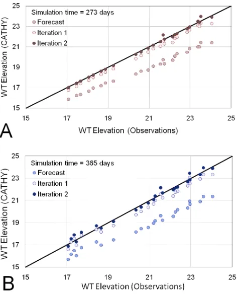
Fig. 17. Comparison between model-calculatedW Tvalues and ob-servedW Tdata from the true system for the forecastW Tensemble, theW T ensemble generated using the updated GM parameter val-ues from the 1st iteration, and theW T ensemble using the updated GM parameters from the 2nd iteration. Comparison are made for

(A) time = 273 days and (B) time = 365 days.

3.3 Case of uncertain geostatistical parameter values

3.3.1 Log-Mean of true YKfield is uncertain

In this section, the ability of the ES update routine to con-dition the ensemble ofYK usingW T observation data

sam-pled from a catchment system whereµYK is different from the one used in generating the forecast ensemble is explored. In the first scenario, µYK of the trueYK field is 1.801 log m day−1 (K= 63.2 m day−1, one-half order of magnitude higher than the forecast value of 20 m day−1); for the sec-ond scenario,µYK of the trueYK field is 0.801 log m day

−1

(K= 6.3 m day−1, one-half order of magnitude lower than the forecast value of 20 m day−1_{). The value ofσ}2

YK in the true systems and the forecast ensemble is the same [(0.250 log m day−1₎2_{]. In Sect. 3.3.2, a more severe test is used to}

demonstrate the iterative approach described in Sect. 2.5. The true YK field for the first and second scenarios are

shown in Fig. 11a and b, respectively. For the two scenar-ios, the AE of the forecastYKensemble is 0.690 and 0.692,

respectively. By assimilatingW T data from 24 observation wells for four assimilation times, the AE of the updatedYK

ensemble for the two scenario is 0.365 and 0.395, respec-tively, resulting in reductions of 47.1 % and 43.0 % from the forecast AE values. The spatial distribution of the up-datedYK ensemble mean for the two scenarios is shown in

Fig. 11c and d. For both scenarios, the updated ensembles capture the general magnitude and spatial distribution of the trueYK field.

For the first scenario, the initially too-low (compared to the true system) values ofYK are conditioned to the higher

values present in the true system; for the second scenario, the initially too-high values are conditioned to the lower values. The same effect is observed through a comparison between the reference, forecast, and updated values ofYK across a

west-east transect located at Y = 2000 m, as shown in Fig. 12. In both scenarios, the forecastYK values along the transect

are approximately equal to the forecastµYK value of 1.301, whereas the updated YK values have been conditioned to

resemble the true profiles.

3.3.2 Iterative approach to discover geostatistical

parameter values

To demonstrate the iterative approach, the true aquifer sys-tem hasµYKandσ

2

YKvalues of 0.301 log m day

−1_{(K= 2.0 m}

day−1_{)and 0.500 (log m day}−1₎2_{. The resulting true Y}

K

field is shown in Fig. 13. For each iteration, observation data from 24 observation wells and four assimilations are used to condition the YK ensemble. Beginning with a forecast

YK ensemble generated usingµYK= 1.301 log m day −1_and

σ_Y2

K= 0.250 (log m day

−1₎2_{, eight iterations are performed,}

with the µYK andσ 2

YK values of the updated YK ensemble after each iteration shown in Fig. 14. As seen in Fig. 14, the value ofµYK reaches the parameter value from the true sys-tem within three iterations, but eight iterations are required to determine if convergence has been achieved. Forσ_Y2

K, the value from the updated YK decreases during the first

sev-eral iterations, but eventually converges upon a value (0.580) slightly higher than the true value of 0.500 (log m day−1)2. If the GM parameter values of the true system were unknown, then it would be assumed thatµYK is just under 0.300 log m day−1andσ_Y2

K is equal to 0.580 (log m day −1₎2_.

Besides the convergence to the true GM parameter values, the approach of the updatedYK ensemble to the spatial

dis-tribution of the trueYKfield is demonstrated in Figs. 15 and

16. The ensemble mean of the updatedYKensemble for

iter-ations 1 through 4 is shown in Fig. 15a–d, with the AE value generally decreasing from the forecast value of 1.106 (0.755, 0.565, 0.507, and 0.518, respectively), although a slight in-crease occurs between iterations 3 and 4. The structure of the YK spatial distribution, however, progressively approaches

the pattern of the trueYK field shown in Fig. 13 with each

successive iteration.

Figure 16 shows the trueYK values, forecastYK values,

and the updated values ofYK for the 1st and 3rd iterations

in the updatedYK values in relation to the trueYK values

occurs from the forecast to the first iteration, and from the first iteration to the third iteration.

Finally, comparisons are made between observedW Tdata from the true system and model-calculatedW T values gen-erated by CATHY using the updated values ofµYK andσ

2

YK from the previous iteration. This is especially important since such a comparison, i.e., re-running the numerical model us-ing the estimated parameter values and comparus-ing model re-sults with observed data at observation locations, is generally the only means by which the parameter estimation method can be verified. Figure 17 shows the comparison between observedW T data and model-calculatedW T values from the forecast ensemble, theW T ensemble generated using the updated GM parameter values from the first iteration, and the W T ensemble using the updated GM parameters from the second iteration. Comparisons for times = 273 days and 365 days are shown in Fig. 17a and b, respectively.

The match between the forecast values and the true value is much improved upon using the results from the first iteration, and an excellent match occurs using the results from the sec-ond iteration. Quantitatively, the sum of squared differences between the model results and true system values is 95.32, 4.29, and 0.59, respectively for time = 273 days, and 99.16, 4.98, and 1.83, respectively for time = 365 days. Notice that the forecastedW T values are lower than the observed W T values from the true aquifer system, since the forecastYK

values are generated using a higher value ofµYK. However, using the lower updated value ofµYK from the first and sec-ond iterations, the W T values become higher and more in accordance with the observedW T values.

4 Conclusions

The ES update routine, a derivative of the Kalman Fil-ter approach, has been evaluated for the estimation of spatially-variableK in a catchment system using the fully-coupled, surface-subsurface flow model CATHY. A 4.05 km by 4.05 km tilted v-catchment was used in demonstration, with spatio-temporal variability in forcing terms to provide increased uncertainty in the system and to strive to mimic real-world conditions.

BothW T data andQ data were collected from a refer-ence catchment system and assimilated into the ensemble of model results to condition the spatial distribution ofKto ap-proach the referenceKfield. AssimilatingW T from a net-work of observation wells provided a distinct improvement in theKensemble in relation to the trueKfield, with sets of data from multiple collection times tempering the decrease in improvement when error was assigned to the observed W T data. AssimilatingQdata only slightly improved the Kensemble in relation to the trueKfield. Jointly assimilat-ingQandW T data only improved the estimate ofK when data from a small number (2,4) of observation wells were

assimilated. This is due to the region of influence ofQ, i.e., the regions of the aquifer where theKvalues directly influ-enceQand hence can be conditioned by observed values of Q, being small compared to the collective region of influence ofW T values at the observation wells.

For cases in which the parameter values defining the geo-statistical structure of the aquifer system are uncertain to a small degree (i.e., mean of trueKfield is one-half order of magnitude different than the assumed mean), the methodol-ogy is still able to condition adequately the forecastK en-semble to approach the magnitude and spatial structure of the true aquifer system. For more severe cases, i.e., the true and assumed means are different by an order of magnitude and the true and assumed variance of theKfield is different, an iterative process using the ES is used to converge upon the true geostatistical parameter values. Results indicate that the process is successful in approximating the true values.

For the present study uncertainty in the correlation length of theKfield is not investigated, and an amendment to the it-erative scheme to converge upon unknown correlation length is left to future research, with assimilation of measurements ofKlikely necessary. Future studies also include an appli-cation of the methodology to an actual catchment system in order to estimate the geostatistical parameter values as well as the spatial distribution ofK.

Acknowledgements. The majority of this work has been made

possible by a Colorado Agricultural Experiment Station (CAES) grant (Project No. COL00690). We kindly thank Gaisheng Liu and an anonymous reviewer for for their helpful comments and suggestions in improving the content of this paper.

Edited by: H. Cloke

References

Ahmed, S. and de Marsily, G.: Cokriged Estimation of Aquifer Transmissivity as an Indirect Solution of the Inverse Problem: A Practial Approach, Water Resour. Res., 29, 521–530, 1993. Aubert, D., Loumagne, C., and Oudin, L.: Sequential assimilation

of soil moisture and streamflow data in a conceptual rainfall-runoff model. J. Hydrol., 280, 145–161, 2003.

Bailey, R. T. and Ba`u, D. A.: Ensemble Smoother assimi-lation of hydraulic head and return flow data to estimate hydraulic conductivity, Water Resour. Res., 46, W12543, doi:10.1029/2010WR009147, 2010.

Bailey, R. T. and Ba`u, D. A.: Estimating spatially-variable first-order rate constants in groundwater reactive transport systems, J. Cont. Hydrol., 122, 104–121, 2011.

Ba´u, D. A. and Mayer, A. S.: Optimal design of pump-and-treat systems under uncertain hydraulic conductivity and plume dis-tribution, J. Cont. Hydrol., 100, 30–46, 2008.

Bennett, A. F.: Inverse Methods in Physical Oceanography, Cam-bridge Univ. Press, New York, 1992.

R. T. Bailey and D. Ba `u: Estimating geostatistical parameters 303

Methods in Water Resources, vol. 2, Computational Methods, Surface Water systems and Hydrology, edited by: Bentley, L. R., Sykes, J. F., Brebbia, C. A., Gray, W. G., and Pinder, G. F., 1115–1122, Balkema, Rotterdam, The Netherlands, 2000. Boulet, G., Kerr, Y., and Chehbouni, A.: Deriving catchment-scale

water and energy balance parameters using data assimilation based on extended Kalman filtering, Hydrol. Sci., 47, 449–467, 2002.

Camporese, M., Paniconi, C., Putti, M., and Salandin, P. :Ensem-ble Kalman filter data assimilation for a process-based catchment scale model of surface and subsurface flow, Water Resour. Res., 45, W10421, doi:10.1029/2008WR007031, 2009.

Camporese, M., Paniconi, C., Putti, M., and Orlandini, S.: Surface-subsurface flow modeling with path-based runoff rout-ing, boundary condition-based couplrout-ing, and assimilation of multisource observation data, Water Resour. Res., 46, W02512, doi:10.1029/2008WR007536, 2010.

Carrera, J. and Neuman, S. P.: Estimation of aquifer parameters un-der transient and steady-state conditions: 1. Maximum likelihood method incorporating prior information, Water Resour. Res., 22, 199–210, 1986.

Carrera, J., Alcolea, A., Medina, A., Hidalgo, J., and Slooten, L. J.: Inverse problem in hydrogeology, Hydrogeol. J., 13, 206–222, 2005.

Chen, Y. and Zhang, D.: Data assimilation for transient flow in ge-ologic formations via Ensemble Kalman Filter, Adv. Water Re-sour., 29, 1107–1122, 2006.

Clark, M. P., Rupp, D. E., Woods, R. A., Zheng, X., Ibbitt, R. P., Slater, A. G., Schmidt, J., and Uddstrom, M. J.: Hydrolog-ical data assimilation with the ensemble Kalman filter: Use of streamflow observations to update states in a distributed hydro-logical model, Adv. Water Resour., 31, 1309–1324, 2008. Dr´ecourt, J.-P., Madsen, H., and Rosbjerg, D.: Calibration

frame-work for a Kalman filter applied to a groundwater model. Adv. Water Resour., 29, 719–734, 2006.

Dunne, S. and Entekhabi, D.: An ensemble-based reanalysis approach to land data assimilation, Water Resour. Res., 41, W02013, doi:10.1029/2004WR003449, 2005.

Durand, M., Molotch, N. P., and Margulis, S. A.: A Bayesian approach to snow water equivalent reconstruction, J. Geophys. Res., 113, D20117, doi:10.1029/2008JD009894, 2008.

Evensen, G.: Using the extended Kalman filter with a multilayer quasi-geostrophic ocean model, J. Geophys. Res., 97, 17905– 17924, 1992.

Evensen, G.: Sequential data assimilation with a nonlinear quasi-geostrophic model using Monte Carlo methods to forecast error statistics, J. Geophys. Res., 99, 10143–10162, 1994.

Evensen, G.: The ensemble Kalman filter: theoretical formula-tion and practical implementaformula-tion, Ocean Dynam., 53, 343–367, 2003.

Evensen, G.: Data assimilation. The Ensemble Kalman Filter, Springer-Verlag Berlin Heidelberg, 2007.

Evensen, G. and van Leeuwen, P. J., An ensemble Kalman smoother for nonlinear dynamics, Mon. Weather Rev., 128, 1852–1867, 2000.

Fu, J. and G´omez-Hern´andez, J. J.: Uncertainty assessment and data worth in groundwater flow and mass transport modeling using a blocking Markov chain Monte Carlo method, J. Hydrol., 364, 328–341, 2009.

Gailey, R. M., Crowe, A. S., and Gorelick, S. M.: Coupled process parameter estimation and prediction uncertainty using hydraulic head and concentration data, Adv. Water Resour., 14, 301–314, 1991.

Gautier, Y. and Nœtinger, B.: Geostatistical parameters estimation using well test data, Oil Gas Sci. Technol., 59, 167–183, 2004. G´omez-Hern´andez, J. J., Hendricks Franssen, H.-J., and Sahuquillo,

A.: Stochastic conditional inverse modeling of subsurface mass transport: A brief review and the self-calibrating method, Stoch. Environ. Res. Risk A., 17, 319–328, 2003.

Hantush, M. M. and Mari˜no, M. A.: Estimation of spatially variable aquifer hydraulic properties using Kalman filtering, J. Hydraul. Engrg. ASCE, 123, 1027–1035, 1997.

Hendricks Franssen, H. J. and Kinzelbach, W.: Real-time groundwater flow modeling with the Ensemble Kalman Fil-ter: Joint estimation of states and parameters and the fil-ter inbreeding problem, Wafil-ter Resour. Res., 44, W09408, doi:10.1029/2007WR006505, 2008.

Hendricks Franssen, H. J. and Kinzelbach, W.: Ensemble Kalman filtering versus sequential self-calibration for inverse modeling of dynamic groundwater flow systems, J. Hydrol., 365, 261–274, 2009.

Hendricks Franssen, H. J., G´omez-Hern´andez, J. J., Capilla, J. E., and Sahuquillo, A.: Joint simulation of transmissivity and stora-tivity fields conditional to steady-state and transient hydraulic head data, Adv. Water Resour., 23, 1–13, 1999.

Hendricks Franssen, H. J., G´omez-Hern´andez, J. J., and Sahuquillo, A.: Coupled inverse modeling of groundwater flow and mass transport and the worth of concentration data, J. Hydrol., 281, 281–295, 2003.

Hoeksema, R. J. and Kitanidis, P. K.: An application of the geo-statistical approach to the inverse problem in two-dimensional groundwater modeling, Water Resour. Res., 20, 1003–1020, 1984.

Hoeksema, R. J. and Kitanidis, P. K.: Analysis of the spatial struc-ture of properties of selected aquifers, Water Resour. Res., 21, 563–572, 1985.

Jafarpour, B. and Tarrahi, M.: Assessing the performance of the ensemble Kalman filter for subsurface flow data integration un-der variogram uncertainty, Water Resour. Res., 47, W05537, doi:10.1029/2010WR009090, 2011.

Kalman, R. E.: A new approach to linear filtering and prediction problems, J. Basic Eng., 82, 35–45, 1960.

Keppenne, C.: Data assimilation into a primitive-equation model with a parallel ensemble Kalman filter, Mon. Weather Rev., 128, 1971–1981, 2000.

Kitanidis, P. K.: On the geostatistical approach to the inverse prob-lem, Adv. Water Resour., 19, 333–342, 1996.

Kitanidis, P. K. and Vomvoris, E. G.: A geostatistical approach to the inverse problem in groundwater modeling (steady state) and one-dimensional simulations, Water Resour. Res., 19, 677–690, 1983.

Li, B. and Yeh, T.-C. J.: Cokriging estimation of the conductiv-ity field under variably saturated flow conditions, Water Resour. Res., 35, 3663–3674, 1999.

Liu, G., Chen, Y., and Zhang, D.: Investigation of flow and transport processes at the MADE site using ensemble Kalman filter, Adv. Water Resour., 31, 975–986, 2008.

method, the ensemble Kalman filter and the ensemble Kalman smoother: A comparison study using a nonlinear reduced gravity ocean model, Ocean Modell., 12, 378–400, 2006.

Orlandini, S. and Rosso, R.: Diffusion wave modeling of distributed catchment dynamics, J. Hydraul. Eng. ASCE, 1, 103–113, 1996. Putti, M. and Paniconi, C.: Time step and stability control for a coupled model of surface and subsurface flow, in Proceedings of the XV International Conference on Computational Methods in Water Resources (CMWR XV), vol. 2, 1391–1402, Elsevier, New York, 2004.

RamaRao, B. S., LaVenue, A. M., de Marsily, G., and Marietta, M. G.: Pilot point methodology for automated calibration of an en-semble of conditionally simulated transmissivity field 1. Theory and computational experiments, Water Resour. Res., 31, 475– 493, 1995.

Reichle, R. H., McLaughlin, D. B., and Entekhabi, D.: Hydrologic data assimilation with the ensemble Kalman filter, Mon. Weather Rev., 130, 103–114, 2002.

Schreider, S. Y., Young, P. C., and Jakeman, A. J.: An application of the Kalman filtering technique for streamflow forecasting in the Upper Murray Basin, Math. Computer Model., 33, 733–743, 2001.

Valstar, J. R., McLaughlin, D. B., te Stroet, C. B. M., and van Geer, F. C.: A representer-based inverse method for groundwater flow and transport application, Water Resour. Res., 40, W05116, doi:10.1029/2003WR002922, 2004.

van Genuchten, M. T. and Nielsen, D. R.: On describing and pre-dicting the hydraulic properties of unsaturated soils, Ann. Geo-phy., 3, 615–628, 1985.

van Leeuwen, P. J. and Evensen, G.: Data assimilation and inverse methods in terms of probabilistic formulation, Mon. Weather Rev., 124, 2898–2913, 1996.

Wen, W.-H., Deutsch, C. V., and Cullick, A. S.: Construction of geostatistical aquifer models integrating dynamic flow and tracer data using inverse technique, J. Hydrol., 255, 151–168, 2002. Woodbury, A. D. and Smith, L.: Simultaneous inversion of

hydro-geologic and thermal data 2. Incorporation of thermal data, Water Resour. Res., 24, 356–372, 1988.

Xie, X. and Zhang, D.: Data assimilation for distributed hydrologi-cal catchment modeling via ensemble Kalman filter, Adv. Water Resour., 33, 678–690, 2010.

Yeh, T.-C. J. and Zhang, J.: A geostatistical inverse method for variably saturated flow in the vadose zone, Water Resour. Res., 32, 2757–2766, 1996.

Yortsos, Y. C. and Al-Afaleg, N.: The permeability variogram from pressure transients of multiple wells: Theory and 1-D applica-tion, Soc. Petrol. Eng. J., 2, 328–337, 1997