www.hydrol-earth-syst-sci.net/14/2559/2010/ doi:10.5194/hess-14-2559-2010
© Author(s) 2010. CC Attribution 3.0 License.
Earth System
Sciences
A multiple threshold method for fitting the generalized Pareto
distribution to rainfall time series
R. Deidda
Dipartimento di Ingegneria del Territorio, Universit`a di Cagliari, Cagliari, Italy Received: 29 June 2010 – Published in Hydrol. Earth Syst. Sci. Discuss.: 23 July 2010 Revised: 31 October 2010 – Accepted: 23 November 2010 – Published: 14 December 2010
Abstract. Previous studies indicate the generalized Pareto
distribution (GPD) as a suitable distribution function to reli-ably describe the exceedances of daily rainfall records above a proper optimum threshold, which should be selected as small as possible to retain the largest sample while assur-ing an acceptable fittassur-ing. Such an optimum threshold may differ from site to site, affecting consequently not only the GPD scale parameter, but also the probability of threshold exceedance.
Thus a first objective of this paper is to derive some ex-pressions to parameterize a simple threshold-invariant three-parameter distribution function which assures a perfect over-lapping with the GPD fitted on the exceedances over any threshold larger than the optimum one. Since the proposed distribution does not depend on the local thresholds adopted for fitting the GPD, it is expected to reflect the on-site cli-matic signature and thus appears particularly suitable for hy-drological applications and regional analyses.
A second objective is to develop and test the Multiple Threshold Method (MTM) to infer the parameters of interest by using exceedances over a wide range of thresholds apply-ing again the concept of parameters threshold-invariance. We show the ability of the MTM in fitting historical daily rainfall time series recorded with different resolutions and with a sig-nificative percentage of heavily quantized data. Finally, we prove the supremacy of the MTM fit against the standard sin-gle threshold fit, often adopted for partial duration series, by evaluating and comparing the performances on Monte Carlo samples drawn by GPDs with different shape and scale pa-rameters and different discretizations.
Correspondence to: R. Deidda ([email protected])
1 Introduction
Several rainfall modelling approaches for hydrological ap-plications use a simple representation of the rainfall process and assume that the marginal distribution of rainy and non-rainy valuesx at daily or any other fixed time scale can be described by the following Cumulative Distribution Func-tion (CDF):
F (x) = Pr{X ≤ x|X ≥ 0} = (1−ζ0) +ζ0F0(x) (1)
x ≥ 0
whereζ0=Pr{X>0|X≥0}represents the probability of
oc-currence of rainy days, whileF0(x)=Pr{X≤x|X>0}is the
CDF of only rainy values.
Commonly used distribution functions F0(x) of strictly
positive rainfall records include the exponential, Gamma (Pearson III), log-Gamma (log-Pearson III), skewed normal (i.e. a normal distribution fitted to the Box-Cox transformed data), and lognormal (e.g., Swift and Schreuder, 1981; Ke-dem et al., 1990a,b, 1997; Shimizu, 1993; Katz, 1999; Cheng and Qi, 2002; Cho et al., 2004; Shoji and Kitaura, 2006; Lan-gousis and Veneziano, 2007; LanLan-gousis et al., 2009; Suhaila and Jemain, 2007).
is fitted on all strictly positive rainfall records and then used to fill in the records of rainy days in the Markov chain (e.g., Nicks, 1974; Nicks et al., 1995; Williams, 1995).
The simple form of Eq. (1) suggests fittingF0(x)on all
strictly positive rainy observations, but particular care should be taken in this (seemingly very simple) approach. Indeed, the distribution of very small values may not be clearly def-inite and may depart from the distribution of the bulk of higher records for several reasons, including: (i) small val-ues may be due to dew processes rather than being the result of true rainfall events; (ii) measurements of very small rain-fall values may be seriously affected by local atmospheric interactions (e.g. evaporation and wind); (iii) small rainfall amounts manually collected by non-recording rain gauges may be sometimes classified as rainy or non-rainy records de-pending on the subjective judgment of the person in charge of the observation. Moreover, whatever the cause may be, there is empirical evidence that small values often depart from the distribution of the bulk of rainfall observations. Thus, what-ever distributionF0(x)is candidate to describe daily rainfall
records, a robust criterion is needed to infer parameter val-ues only on records exceeding a proper optimum threshold, in order to be confident that all the censored values belong to the same distribution.
We also want to highlight that fitting a distribution func-tion Fu(x)=Pr{X≤x|X>u} on the records above a given
thresholduleads in general to parameter estimates that differ from those ofF0(x), even ifF0(x)andFu(x)belong to the
same family. For practical applications it is thus particularly useful to derive relationships to parameterize Eq. (1) with threshold-invariant parameters by assuring a perfect overlap-ping with the distributionFu(x)for anyx>u, regardless the
value of the thresholdu.
The first objective of our work is thus the derivation of such relations. Although some developments presented in this paper hold for any distribution function Fu(x),
we specifically focus on the generalized Pareto distribu-tion (GPD) (Pickands, 1975) for the following reasons.
First, under certain conditions, the GPD family has impor-tant connections with the generalized extreme value distri-bution (GEV) family (e.g. the shape parameter is expected to be the same asymptotically as the thresholdu→ ∞, while the other parameters are linked through theoretical relations), thus fitting GPD can give us a more accurate insight into the maxima. Referring the reader to Gumbel (1958), Castillo (1988), and Coles (2001) for a review of the GEV and GPD properties and derivations, we just remark that if there exists a limiting distribution of the block-maxima extracted from our samples (usually yearly maxima in Earth sciences), this distribution belongs to the domain of attraction of the GEV family (Fisher and Tippett, 1928; Gnedenko, 1943). In ad-dition, under these conditions, the Balkema – De Haan – Pickands theorem (Balkema and de Haan, 1974; Pickands, 1975) states that the limit distribution of scaled excesses over high enough thresholds has a corresponding approximate
distribution within the GPD family. For hydrological ex-treme events modelling, Madsen et al. (1997a,b) general-ized previous findings by Cunnane (1973) and showed that fitting a GPD on a reasonable number of exceedances over a proper threshold leads to more accurate extreme quantile estimates than fitting a GEV on annual maxima. We re-mark also that it would be desiderable to select as low an optimum threshold as possible in order to minimize the es-timation variance when fitting the GPD on observed sam-ples (Coles, 2001). With this aim, graphical and numerical methods have been proposed and applied by several authors (e.g., Davison and Smith, 1990; Smith, 1994; Lang et al., 1999; Dupuis, 1998; Choulakian and Stephens, 2001; Guil-lou and Hall, 2001; Peng and Qi, 2004), but what can be assumed as an optimal threshold for rainfall observations is still an open question without a definitive answer. In a recent study, under the hypothesis that the rainfall process can be described by multiplicative models, Veneziano et al. (2009) highlighted some convergence problems for the GPD shape parameter when fitting the distribution function on records above a finite threshold. Finally, the detection of an optimum threshold becomes even more difficult, if not impossible us-ing available methods, on heavily quantized records (Deidda and Puliga, 2006). In this framework, the GPD fitting ap-proach proposed in this paper makes it possible to overcome some of these problems, such as the estimation bias related to heavily quantized records and to non asymptotic thresholds (Veneziano et al., 2009).
A second reason for the adoption of the GPD is that its mathematical form leads to very simple equations for the pa-rameterization of Eq. (1) using results of inference on records censored with any threshold. Indeed, for thresholds larger than the optimum, the shape parameter of the GPD is ex-pected to be constant, while the scale parameter should lin-early depend on the threshold value. Thus simple linear equations for reparameterization of the scale parameter have been proposed (see e.g., Madsen et al., 1997b; Coles, 2001). Beguer´ıa (2005) analyzed several daily time series in Spain and used these expressions to estimate the scale parameters corresponding to the on-site optimum thresholds by averag-ing the reparameterized scale values obtained for a range of thresholds. Nevertheless, a drawback of this approach is that the final scale parameter estimates depend not only on the local climatic conditions but also on the on-site optimum threshold. In this paper we generalize these concepts in or-der to eliminate the dependence of the scale parameter on the threshold and we also provide a threshold-invariant pa-rameterization for theζ0parameter. Specifically, we rewrite
As the last but not least reason, there is much published evidence of the good capability of the GPD in describing rainfall exceedances (see e.g., Cameron et al., 2000; Coles et al., 2003; De Michele and Salvadori, 2005; Fitzgerald, 1989; Madsen et al., 2002; Salvadori and De Michele, 2001; Van Montfort and Witter, 1986). Moreover, recent studies by Beguer´ıa (2005), Deidda and Puliga (2006), and Beguer´ıa et al. (2009) gave evidence, using L-moment ratio diagram (Hosking, 1990), that GPD is the best candidate to be the parent distribution of daily rainfall time series.
The second objective of this paper is to propose and test the Multiple Threshold Method (MTM) which is based on the threshold-invariant GPD parameterization of Eq. (1) and provides a fitting to Eq. (1) on the excesses above a proper range of thresholds. Although the motivation for the de-velopment of the MTM comes from the need to improve the fitting on irregularly discretized records, as is often the case for manually collected rainfall measurements, we show that its performances are superior anyway to standard single-threshold fitting on regularly discretized data. The need of such a technique is motivated by the discretization usually adopted for rainfall records, which can be the common stan-dard resolution of 0.2 mm for tipping-bucket rain gauges in Europe (or 0.254 mm in the US), but can also become higher for records manually collected by non-recording rain gauges. For example, Deidda (2007) highlighted that many time series collected by the Sardinian Hydrological Survey (Italy) contain anomalous quantities of daily rainfall records rounded off at unexpected resolutions of 0.5, 1 and 5 mm/d. Recently, Deidda and Puliga (2009) evaluated and compared the performances of several estimators of the GPD param-eters on discretized samples. Specifically, they considered some widely used estimators such as those based on maxi-mum likelihood, simple moments and probability weighted moments (Hosking and Wallis, 1987), as well as other re-cently proposed GPD estimators such as those based on the maximum penalized likelihood (Coles and Dixon, 1999), the minimum density power divergence (Ju´arez and Schucany, 2004), the likelihood moment estimator (Zhang, 2007), the median estimator (Peng and Welsh, 2001). Nevertheless, Deidda and Puliga (2009) concluded that none of the con-sidered methods provides acceptable estimates when records are discretized at a resolution of 1 mm or larger. Indeed bias and root mean square errors of parameter estimates are often of the same magnitude as the site-to-site variability of the pa-rameter values to be estimated. In this paper we show, using observed as well as synthetic time series, how the Multiple Threshold Method is able to overcome these fitting problems even on roughly rounded-off and heavily quantized records.
The paper is organized as follows. Section 2 briefly describes the database. In Sect. 3, we derive some rela-tions between Eq. (1) and distribution funcrela-tions fitted on the exceedances above any threshold, then we provide spe-cific equations to reparameterize the GPD and finally rewrite Eq. (1) with only three threshold-invariant parameters. In
Sect. 4, we introduce the MTM and present some examples of application on daily rainfall time series. In Sect. 5, the per-formances of the MTM are evaluated on Monte Carlo sam-ples drawn by GPD, while Sect. 6 is devoted to the conclu-sions.
2 Database
Some of the analyses and figures presented in the follow-ing sections were performed on daily rainfall time series collected by the Sardinian Hydrological Survey (Italy) from 1922 to 1996: specifically, we used 217 time series with more than 40 complete years of records. Most of the se-ries were collected by non-recording standard rain gauges and discretized with resolutions up to 1 and 5 mm (Deidda, 2007), while only a subset was obtained by tipping-bucket rain gauges and was correctly discretized at 0.2 mm. Time series are used with a twofold objective: to show the MTM working on historical records and to select representative GPD parameters for evaluation of MTM performances on synthetic samples.
3 Some basic relationships
We derive here some general relationships among the marginal distributionF (x)in Eq. (1) and distribution func-tions Fu(x) of the exceedances over any threshold u≥0
(Sect. 3.1). Results are then applied to parameterize Eq. (1) using GPD parameter estimates on left-censored records in order to obtain a three-parameter distribution which de-scribes rainy and non-rainy values (Sect. 3.2). A reader who is not interested in the details of derivation of such relation-ships may skip Sect. 3, just keeping in mind Eqs. (8) and (9), which are needed to reparameterize the GPD in Eq. (10) us-ing estimates obtained with any thresholdu.
3.1 Some relations among uncensored and left-censored
distribution functions
We want first to derive some relationships amongF (x)= Pr{X≤x|X≥0}, F0(x)=Pr{X≤x|X>0}, and Fu(x)=
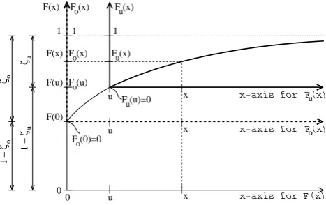
Pr{X≤x|X>u}, in order to obtain a perfect overlapping among these Cumulative Distribution Functions (CDFs) for anyx>uas sketched in Fig. 1.
Using simple arguments of probability we can write Fu(x)=1−Pr{X>x|X>u} =1−PrPr{{X>xX>u||XX≥≥00}}=1−11−−F (x)F (u)
forx>u. These equalities lead to the following relationship betweenF (x)andFu(x)for anyx>u:
F (x) = (1 −ζu) +ζuFu(x) x > u (2)
whereζu=Pr{X>u|X≥0}=1−F (u) represents the survival
F (x)u
F (u) o F (x)o
F (u)=0u
o
ζ
o
1 − ζ
u
ζ
u
1 − ζ
F (x)u F (x)o
F (0)=0o F(x)
0 F(u)
F(0)
0
1 1 1
F(x)
u
u
u
x−axis for
x−axis for F(x) x−axis for x
x
x
F(x)u
[image:4.595.50.284.63.210.2]F(x)o
Fig. 1. The sketch depicts some relations among the cu-mulative distribution functions (CDFs) F (x)=Pr{X≤x|X≥0},
F0(x)=Pr{X≤x|X>0}, and Fu(x)=Pr{X≤x|X>u}, which are
used in the text to determine the constraints for overlapping of all the CDFs for anyxabove the thresholdu. Cartesian axes ofF (x)
are drawn with a thin line and characteristic values are reported on the left side, while the axes ofF0(x)and Fu(x)are drawn with
dashed and solid thick lines, respectively, with values reported on the right side.
Fu(u)=limx→u+Fu(x)=0, Eq. (2) becomes valid for any x≥uand thus includes also Eq. (1) as a special case foru=0.
Using similar arguments we can write Fu(x)=1−Pr
{X>x|X>0}
Pr{X>u|X>0}=1−
1−F0(x)
1−F0(u) to obtain a relationship
betweenF0(x)andFu(x):
F0(x)= F0(u) + [1 −F0(u)]Fu(x) x ≥ u (3)
Finally, computing Eqs. (1) and (2) for x=u, eliminating F (u)among the equations, and puttingFu(u)=0 we obtain:
ζu = ζ0[1 −F0(u)] (4)
We highlight that all the above equations hold for any distri-bution functionFu(x)adopted to fit the exceedances above a
thresholdu. The same equations can be derived by the fol-lowing proportions in Fig. 1:
1−F (x) 1−F (u) =
1 −F0(x)
1 −F0(u)
= 1 −Fu(x) 1 −Fu(u)
x > u (5)
3.2 GPD reparameterization
Now let us assume that for a given threshold u the ex-ceedances of our sample could be reliably described by a generalized Pareto distribution (GPD):
Fu(x) = Fu (x;αu, ξ ) = (6)
=
1 −
1 +ξ xα−u
u −1/ξ
ξ 6= 0 1 − exp −x−u
αu
ξ = 0
whereξ is the shape parameter,αuthe scale parameter, while
uis the threshold value.
Theξ parameter controls the tail behaviour of the distri-bution and the attitude to originate heavy extremes. Forξ=0 the distribution has the ordinary exponential form. Forξ >0 the distribution has a long right tail, thus it is often referred to as “heavy tailed distribution”: in this case it is worth noticing that simple moments of order greater than or equal to 1/ξare degenerate, thus estimators based on ordinary moments can be applied to fit Eq. (6) only forξ1/2 to prevent degenera-tion of the first two moments and consequent parameter esti-mation biases (Hosking and Wallis, 1987). Forξ <0 the dis-tribution is short tailed with an upper bound value(u−αu/ξ ).
For a givenξ, the scale parameterαucontrols the mean of the
exceedances above the thresholdu. Finally, the thresholdu cannot be considered a true distribution parameter: indeed, the value ofumust be specified (and used for left-censoring the sample) before fitting Eq. (6) since the GPD is a distribu-tion of threshold excesses.
As discussed in the Introduction, in literature several meth-ods have been proposed to infer the shapeξ and the scaleαu
parameters of the GPD once the threshold u has been set. Concerning the probabilityζu to observe an exceedance of
the thresholdu, since the number of exceedances follows a binomial distribution, the same following estimator can be derived by the maximum likelihood, the simple moments, and the probability weighted moments methods:
ζu =
Nu
N (7)
whereNuis the number of records above the thresholduand
Nis the sample size (including the zeros).
The generalized Pareto distribution has an important prop-erty. If a sample can be reasonably considered drawn by a GPD with thresholdu∗and shape parameterξ, then the ex-cesses of any other thresholdu>u∗should also follow a GPD with the same shape parameterξ and a scale parameterαu
which will linearly change with the thresholdu.
Now, let us assume that GPD in Eq. (6) is a reasonable model for the exceedances over a given threshold u and that parametersξ,αu andζuhave been estimated using
ex-ceedances over this threshold. Our objective is to parame-terize equationsF (x)andF0(x)by imposing a perfect
over-lapping withFu(x)for anyx>u, as depicted in Fig. 1 and
formalized by the equations derived in Sect. 3.1. In doing so let us assume that alsoF0(x)is a GPD with thresholdu=0
and parameters α0 andξ, and that it can be expressed by
Eq. (6) withu=0.
SubstitutingF0(x)andFu(x)from Eq. (6) into Eq. (3) we
can easily obtain:
α0 = αu −ξuu ∀ξu (8)
Thus, if a suitable threshold has been selected (so that the excesses can be reliably represented by a GPD), by virtue of Eq. (8) theα0reparameterization should be invariant for any
higher threshold (even ifαu changes withu). As discussed
in the introduction, similar equations have been proposed and used to reparameterize the scale parameterαu∗ correspond-ing to the optimum thresholdu∗ by usingαu estimates
ob-tained for thresholdsu>u∗(see e.g., Madsen et al., 1997b; Beguer´ıa, 2005). Nevertheless, in such approachesαu∗ esti-mates will depend not only on the local climatic conditions but also on the local optimum thresholdu∗, which may be different from site to site. In contrast, results from Eq. (8) do not depend on the on-site optimum threshold. Finally we highlight that Eq. (8) can also be derived by the linkage be-tween GPD and GEV distribution in the asymptotic limit (see e.g., Coles, 2001, p. 83), but here it was obtained more sim-ply without this assumption.
Computing nowF0(u)from Eq. (6), i.e. putting firstu=0
and then computing forx=u, substituting F0(u)in Eq. (4),
and (optionally) using Eq. (8) we obtain:
ζ0 =
ζu
1+ ξuαu0
1/ξ
= ζu
1−ξuαuu
−1/ξ
ξu 6=0
ζuexpαu0 =ζuexp αuu ξu = 0
(9)
As Eq. (8), this last equation states that theζ0
reparameter-ization is threshold-invariant, although the probabilityζu of
exceedinguobviously decreases asuincreases.
Finally, a threshold-invariant GPD parameterization is ob-tained by substitutingF0(x)from Eq. (6) into Eq. (1), and
usingα0andζ0values calculated from Eqs. (8) and (9):
F (x) =
1 −ζ0
1 +ξ αx
0
−1/ξ
ξ 6= 0 1 −ζ0exp
−x
α0
ξ = 0
x ≥ 0 (10)
Assuming x as an i.i.d. random variable, the distri-bution function of annual maxima G(x) is related to F (x) and the yearly return period T by the relation G(x)=F (x)n=1−1/T, where n=365.25 is the average number of days in a year. Thus obtaining an expression for theT-year return period quantile is straightforward:
xT =
α0
ξ
"
1−
1−T1
1/n
ζ0
#−ξ
−1
ξ 6= 0
−α0ln
"
1−
1−T1
1/n
ζ0
#
ξ = 0
(11)
We highlight two important properties of Eq. (10). Firstly, it perfectly overlaps any GPD fitted on the exceedances over thresholds larger than the optimum oneu∗: the only minor drawback is that there can be small departures from records smaller than u∗, but this does not affect extreme quantile estimations by Eq. (11). Secondly, the three parameters in
Eq. (10) do not depend on the threshold used for GPD fit-ting, but only on the local climatic features: this property is particularly helpful to investigate the spatial pattern of rain-fall signature in regional analyses.
4 The multiple threshold method
By virtue of the GPD properties and of the derivations pre-sented in Sect. 3, if a sample can be reasonably considered drawn from a GPD with threshold u∗ and shape parame-tersξ, then for any other thresholdu>u∗we should expect threshold-invariance not only for the estimates of the shape parameterξ, but also for the reparameterizationsα0andζ0
provided by Eqs. (8) and (9). This concept is used in the de-velopment of the Multiple Threshold Method (MTM) which is based on the parameter estimates within a range of thresh-oldsu>u∗and provides robust GPD fitting regardless of the data resolution or rounding off. Concerning the choice of the optimum thresholdu∗we remark that it should be selected large enough to reliably consider the distribution of the ex-ceedances closely approximated by a GPD, but low enough to keep small the estimation variance.
For the sake of clarity, we first present in Sect. 4.1 the MTM with an application on a time series in our database which was recorded at 0.2 mm resolution, deferring the prob-lems related to data discretization and MTM application on roughly rounded-off records to Sect. 4.2.
4.1 MTM rationale
To show how the threshold-invariant properties of the param-eterizations derived in Sect. 3 hold for rainfall time series and to convey better the MTM rationale, in Figs. 2 and 3 we present the results obtained on a 58-yr long time series recorded by a tipping-bucket rain gauge at a 0.2 mm resolu-tion.
We first obtained theξandαuestimates on the excesses of
a range of thresholdsuby maximizing the likelihood func-tion in Grimshaw (1993), and the ζu estimates by Eq. (7).
Then we used Eqs. (8) and (9) to calculate the parametersα0
andζ0for each thresholdu. The first three plots from the top
of Fig. 2 show these estimatesξ,α0andζ0as a function of
thresholdsuranging from 0 to 20 mm. We can clearly ob-serve a stabilization of theξ estimates for thresholds larger thanu∗≈3 mm, indicating that the tail behaviour becomes stable and thusu∗can be considered an optimal threshold. A similar behaviour can be observed for the estimates ofα0and
ζ0which become stable foru>u∗, as expected by the
theo-retical derivations presented in previous Sect. 3. Finally, for thresholds larger than about 10 mm, we can observe all the estimates starting to visibly fluctuate, and moreover the devi-ations of theξ parameter seem to be amplified in theα0and
ζ0estimates. We also remark that the increasing variability
0 5 10 15 20 0
0.2 0.4
ξ
(u)
ML−MTM−GPD fit st074−58y ξM = 0.15 − α 0
M = 4.95 − ζ 0 M = 0.20
0 5 10 15 20
0 5 10 15
α0
(u)
0 5 10 15 20
0 0.5
ζ0
(u)
0 5 10 15 20
0 5 10 15
α 0
C(u)
0 5 10 15 20
0 0.5
ζ0 C (u)
0 5 10 15 20
0 2 4 6
N(x>u) / 1000
[image:6.595.314.545.68.448.2]u [mm]
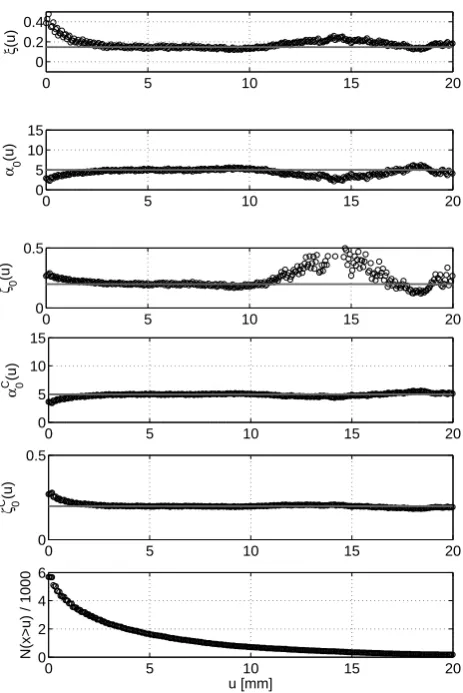
Fig. 2. Example of MTM application on a daily rainfall time series
collected by a tipping-bucket rain gauge with a 0.2 mm resolution. The first plot from the top displays theξestimates as the thresholdu
ranges from 0 to 20 mm: theξMMTM estimate is the median value (horizontal line) within the range of thresholds between 2.5 and 12.5 mm suggested for practical applications. Similarly, the sec-ond and third plots display the uncsec-onditionedα0andζ0estimates
provided by Eqs. (8) and (9) as a function ofu. In the fourth plot the
α0MMTM estimate is obtained as the median value of the reparam-eterizedαC0 estimates conditioned to theξMMTM estimate, while in the fifth plot theζ0MMTM estimate is obtained by theζ0C esti-mates conditioned to bothξMandαM0 MTM estimates. The sixth plot shows the sizes of the records exceeding the thresholdsu. The starting point of stabilization of all estimates suggestsu∗≈3 mm as an optimum threshold.
that thresholds between 10 and 20 mm may be considered modest, the corresponding number of exceedances becomes very small, as shown in the last plot of Fig. 2.
Although the rigorous assessment of the optimum thresh-oldu∗ goes beyond the main scope of this paper, we per-formed the same analysis on the other time series that were
0 20 40 60 80 100
10−5 10−4 10−3 10−2 10−1 100
x [mm] − daily rainfall
log
10
[1−F(x)]
ML−MTM−GPD fit st074−58y ξM = 0.15 − α0M = 4.95 − ζ0M = 0.20
sample
ML−MTM−GPD fit
0 5 10 15 20 25 30
0.7 0.75 0.8 0.85 0.9 0.95 1
x [mm] − daily rainfall
F(x)
ML−MTM−GPD fit st074−58y ξM = 0.15 − α 0
M = 4.95 − ζ 0 M = 0.20
sample
ML−MTM−GPD fit
Fig. 3. These figures display the good GPD fitting obtained by MTM application showed in Fig. 2. The top plot shows the em-pirical survival function (circles) and Eq. (10) parameterized with MTM estimates (line): we can observe how the fitting can reliably capture the highest records, despite the fact that the MTM was ap-plied with a moderate range of thresholds up to 12.5 mm. The bot-tom plot shows a zoom of the empirical CDF and the MTM-GPD fit with the same symbols: we can observe again a good fitting, ex-cept for very small records below the optimum thresholdu∗≈3 mm detected in previous Fig. 2.
recorded with a 0.2 mm discretization. The results were very similar to those presented in Fig. 2, revealing the the optimal thresholdu∗in our dataset is always smaller than 5 mm and generally around 3–4 mm.
Starting from these observations and from the results on roughly discretized time series presented in Fig. 4 and discussed later, the main idea of the Multiple Threshold Method (MTM) is to estimate theξ, α0 andζ0 parameters
[image:6.595.51.283.87.434.2]0 5 10 15 20 0 0.2 0.4 ξ (u)
ML−MTM−GPD fit st007−56y ξM = 0.03 − α 0 M = 8.51 − ζ
0 M = 0.21
0 5 10 15 20
0 5 10 15 α0 (u)
0 5 10 15 20
0 0.5
ζ0
(u)
0 5 10 15 20
0 0.2 0.4
ξ
(u)
ML−MTM−GPD fit st285−60y ξM = 0.25 − α 0 M = 7.92 − ζ
0 M = 0.25
0 5 10 15 20
0 5 10 15 α0 (u)
0 5 10 15 20
0 0.5
ζ0
(u)
0 5 10 15 20
0 0.2 0.4
ξ
(u)
ML−MTM−GPD fit st368−57y ξM = 0.36 − α 0 M = 6.49 − ζ
0 M = 0.20
0 5 10 15 20
0 5 10 15 α0 (u)
0 5 10 15 20
0 0.5
ζ0
(u)
0 5 10 15 20
0 5 10 15 α0 C(u)
0 5 10 15 20
0 0.5
ζ0 C(u)
0 5 10 15 20
0 2 4 6
N(x>u) / 1000
u [mm]
0 5 10 15 20
0 5 10 15 α0 C(u)
0 5 10 15 20
0 0.5
ζ0 C(u)
0 5 10 15 20
0 2 4 6
N(x>u) / 1000
u [mm]
0 5 10 15 20
0 5 10 15 α0 C(u)
0 5 10 15 20
0 0.5
ζ0 C(u)
0 5 10 15 20
0 2 4 6
N(x>u) / 1000
u [mm]
0 20 40 60 80 100 120
10−5 10−4 10−3 10−2 10−1 100
x [mm] − daily rainfall
log
10
[1−F(x)]
ML−MTM−GPD fit st007−56y ξM = 0.03 − α 0 M = 8.51 − ζ
0 M = 0.21
sample ML−MTM−GPD fit
0 50 100 150 200 250
10−5 10−4 10−3 10−2 10−1 100
x [mm] − daily rainfall
log
10
[1−F(x)]
ML−MTM−GPD fit st285−60y ξM = 0.25 − α 0 M = 7.92 − ζ
0 M = 0.25
sample ML−MTM−GPD fit
0 50 100 150 200 250 300 350
10−5 10−4 10−3 10−2 10−1 100
x [mm] − daily rainfall
log
10
[1−F(x)]
ML−MTM−GPD fit st368−57y ξM = 0.36 − α 0 M = 6.49 − ζ
0 M = 0.20
[image:7.595.59.538.62.441.2]sample ML−MTM−GPD fit
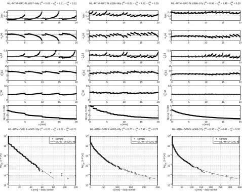
Fig. 4. Other examples of application of the MTM estimator as in Fig. 2, but here columns show the results on time series containing anomalous percentages of roughly rounded-off records. The selection of the time series was made to give examples of MTM working with different roundings (the left column shows results for a sample with many records discretized at 5 mm, the other ones for samples containing many roundings at 1 mm) and different values of the shape parameter (from left to rightξ≈0, 0.25, 0.35). Again, comparing the fourth row of subplots against the second one, and the fifth one against the third one we can observe the benefit of hierarchical MTM application. Finally the last row compares the empirical survival function (circles) with Eq. (10) parameterized withξM,α0Mandζ0MMTM estimates (line) for each time series.
we suggest the adoption of the median value since it is quite robust to the asymmetric distribution of the estimates ob-tained for different thresholds on discretized samples (see e.g., Fig. 4). Concerning the range of thresholds to be adopted, we calculate the median of the estimates obtained for thresholds ranging from 2.5 to 12.5 mm: for our time se-ries this represents a trade-off among the need to (i) have a range large enough to filter out and smooth the departures ar-tificially driven by large roundings (as those shown in the left column of Fig. 4), (ii) hold enough exceedances in order to keep small the estimation variance, and (iii) perform almost all the estimates using thresholdsu>u∗.
The horizontal lines of the first three plots in Fig. 2 show preliminary MTM results, i.e. the median of theξ,α0andζ0
estimates on a range of thresholdsufrom 2.5 to 12.5 mm. We can observe how the parameter estimates within the adopted range of thresholds are very close to the lines representing the MTM estimates. The departures on the left hand side indi-cate that the exceedances over thresholds smaller than 3 mm are not fitted by a GPD, while the departures observed for the larger thresholds are due, as already discussed, to the increas-ing estimation variance associated with the small number of exceedances.
the following hierarchical steps, where the final MTM esti-mates will be denoted asξM,α0M, andζ0Mand will be used to parameterize Eq. (10).
– Step 1:ξMestimate. We first obtain the MTM estimate
ξMof the shape parameter as the median of theξ esti-mates on the suggested range of thresholds as shown in first plot of Fig. 2.
– Step 2:α0Mestimate. In order to filter out the variability
of theα0 estimates driven by the fluctuations ofξ we
estimate again theαuvalues conditioned toξMestimate
obtained at step 1 (i.e. we maximize the likelihood func-tion withξ=ξMknown) and use again the reparameter-ization in Eq. (8) with the newαuestimates andξ=ξM
constant. Results from Eq. (8) are now denoted asα0Cto remark that they are conditioned toξMand are shown in the fourth plot of Fig. 2: comparing with the second plot of the same figure we can observe a minor dispersion of the newαC0 estimates. Finally, the MTM estimateαM0 of the scale parameter is the median of the newα0C esti-mates within the range of thresholds.
– Step 3: ζ0M estimate. In a similar way we can reduce
the variability ofζ0by introducing theζuestimates
pro-vided by Eq. (7) together with the MTM estimatesξM andα0M(obtained at step 1 and 2) into Eq. (9). Results from Eq. (9) are now denoted asζ0Cto remark again that they are conditioned toξMandαM0 and are shown in the fifth plot of Fig. 2 which again displays a reduction of variability with respect to the unconditioned estimates in the third plot of the same figure. Finally, the MTM es-timateζ0Mis the median of the newζ0Cestimates within the range of thresholds.
The described procedure provides the MTM estimates ξM=0.15, α0M=4.95 mm, and ζ0M=0.20 that are used to parameterize Eq. (10) for the analyzed time series. Fig-ure 3 (top) shows the excellent fitting of Eq. (10) to our sample from moderate to the highest rainfall values, while Fig. 3 (bottom) provides a zoom of the empirical CDF to show departures from very small rainfall values, consistently with results of parameter estimates presented in previous Fig. 2. However, adopting the optimal thresholdu∗≈3 mm, with the exception of the recordsx∈(0,u∗), Eq. (10) allows modelling in a simple way (i.e. with only three threshold-invariant parameters) the whole rainfall marginal distribution and gives a very good representation of the higher records providing a reliable insight on the extreme behaviour.
4.2 MTM on roughly rounded-off records
We want now to discuss the MTM application on time se-ries with significant percentages of records rounded off at large discretizations. Deidda (2007) analyzed the database described in Sect. 2 and found that many daily rainfall time
series collected by non-recording rain gauges contain anoma-lous percentages of records discretized at multiples of 0.1, 0.2, 0.5, 1 and 5 mm. Columns from left to right in Fig. 4 show the results of the MTM on three of these time series with different discretizations and shape parameter values: the first time series contains more than 30% of records anoma-lously discretized at multiples of 5 mm and is characterized byξ≈0; the second one has about 70% of records discretized at 1 mm andξ≈0.25; the third one counts about 35% of val-ues at 1 mm resolution andξ≈0.35.
As in Fig. 2, the first three rows of subplots in Fig. 4 show theξ,α0, andζ0estimates as a function of the thresholdu.
If we compare these results with those presented in Fig. 2 we can observe an increased dispersion and a wide spread of all the estimates, and we can also observe the repetition of some patterns at multiple intervals of the discretizations of the records. The fourth and fifth rows show the condi-tioned estimatesαC0 andζ0C: we can observe a stabilization of these estimates, although the signatures of roundings are still present. As previously described, the MTM estimates ξM,α0M, andζ0M are obtained as the median ofξ,αC0, and ζ0C values (displayed in the first, fourth and fifth rows of subplots in Fig. 4) within the range of thresholds between 2.5 and 12.5 mm.
Analyzing the results of Fig. 4, it should now be clearer the rationale of our suggestion to apply the MTM in a range of thresholds between 2.5 and 12.5 mm. Indeed, since we often observed an anomalous percentage of roundings with 5 mm resolution, the adopted range corresponds to joining two in-tervals of thresholds of 5 mm in size and centered on 5 mm and 10 mm, where we observe the jumps of the estimates. At the same time applying the median operator to the estimates on the proposed range of thresholds should guarantee that the MTM estimates are not affected by errors due to an impre-cise location of the optimal thresholdu∗. Indeed, we can also notice how determining the optimal thresholdu∗by looking for the starting point of constant parameter estimates is quite difficult, if not impossible here.
Finally the last row of Fig. 4 compares the empirical sur-vival functions of the three time series with Eq. (10) param-eterized by the MTM estimatesξM,α0M, andζ0M. As already noticed for Fig. 3 we can observe again the good perfor-mances of the MTM in capturing the tail of the empirical distributions, despite the roundings. Thus, regardless of the exponential or heavy tailed shape behaviour, the proposed approach is robust also when fitting time series with signif-icant percentages of roughly rounded-off and heavily quan-tized records.
5 MTM performances
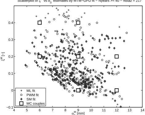
results with those of a standard fit with a single threshold. In order to evaluate the performances on synthetic samples that can be considered representative of our daily rainfall records, we preliminarily evaluated the GPD parameters on the longest time series belonging to the dataset described in Sect. 2: namely, 217 time series with more than 40 com-plete years of records. With this aim, the MTM presented in Sect. 4 was first applied on these time series with a range of thresholds between 2.5 and 12.5 mm and using three differ-ent GPD parameters estimators: the Simple Momdiffer-ents (SM), the Probability Weighted Moments (PWM), and the Maxi-mum Likelihood (ML) methods based on the expression re-ported in Hosking and Wallis (1987), Stedinger et al. (1993), and Grimshaw (1993). The MTM estimates ofξM andαM0 parameters obtained for each station using the three estima-tors are shown in the scatterplot of Fig. 5. We can observe how theξMestimates derived from the SM method are never larger than 0.35: this can be explained by the bias of the estimator related to the divergence of ordinary moments on heavy tailed distributions (Hosking and Wallis, 1987), thus we discarded the SM approach for our analysis. We can also observe that theξMestimates by ML are slightly more spread than the PWM ones. We investigated the issue to some de-tail and the largest ML estimates should be due to the higher sensitivity of the ML method to the presence of outliers or to convergence problems as argued by Hosking and Wallis (1987). We also visually inspected the CDFs of the few time series with a negative shape parameter and found that they can be reliably described by exponential distributions (ξ=0). On the basis of this preliminary analysis, we decided to explore the MTM performances with the ML estimator on Monte Carlo samples generated by Eq. (10) with the follow-ing 7 couples (ξ,α0) of GPD parameters (displayed in Fig. 5
with square symbols): (0, 9), (0, 12), (0.2, 6), (0.2, 9), (0.2, 12), (0.4, 6), (0.4, 9).
90% of the MTMζ0M estimates resulted in a range be-tween 0.15 and 0.25 with a median value very close to 0.20, while the lengths of the considered time series range between 40 and 60 yr. Thus, for the sake of simplicity, we decided to generate all synthetic daily rainfall time series by Eq. (10) us-ing only the valueζ0=0.20 and a length of 50 yr, since
choos-ing different values has the only effect to slightly change the number of strictly positive records.
To evaluate the MTM performances on records with dif-ferent discretizations we considered the following groups of tests:
– Test A: all records are discretized with a 0.2 mm
reso-lution. This corresponds to the standard resolution of most tipping-bucket rain gauges in Europe.
– Test B: all records are discretized with a 1 mm
resolu-tion, as most time series in our database contain large amounts of records discretized at multiples of 1 mm.
4 5 6 7 8 9 10 11 12 13 14
−0.1 0 0.1 0.2 0.3 0.4
α0 M
[mm]
ξ
M [−]
Scatterplot of ξM
vs α0
M
estimates by MTM−GPD fit − Nyears >= 40 − Nstaz = 217
[image:9.595.310.546.67.254.2]ML fit PWM fit SM fit MC couples
Fig. 5. The scatterplot displays the couples of (ξM, α0M) MTM estimates of GPD parameters for the 217 daily rainfall time series (which are more than 40-yr long) collected by the Sardinian Hy-drological Survey (Italy). Parameters estimates were obtained by applying the MTM within a range of thresholds between 2.5 and 12.5 mm: plus signs, circles, and diamonds refer to estimates based on maximum likelihood (ML), probability weighted moments (PWM) and simple moments (SM), respectively. Finally the seven couples of GPD parameters used in Sect. 5 to explore the perfor-mances of the MTM on Monte Carlo samples are drawn with square symbols.
– Test C: 30% of records are discretized with a 5 mm
res-olution, 40% are discretized with a 1 mm resres-olution, while the remaining 30% are discretized at 0.2 mm. This is the case of a large number of time series in which we detected a mixture of discretizations up to 5 mm. In summary, we generated 5000 samples of 50-yr synthetic daily rainfall time series from Eq. (10) with a probability of rainfallζ0=0.20 and (ξ,α0) parameters taking the values of
the 7 couples reported above. Each sample was then dis-cretized according to the three group of tests.
On each sample we estimated theξ, α0, andζ0
parame-ters with two different approaches. In the first approach the ξ andα0values are simply estimated on all strictly positive
records, thus adopting a single thresholdu=0, whileζ0is
es-timated as the ratio between the number of all strictly positive records and the sample size: this will be referred to as “stan-dard fit”. In the second approach theξ,α0, andζ0parameters
are provided by the MTM on a range of thresholds between 2.5 and 12.5 mm as described in Sect. 4: this approach will be referred to as “MTM fit”. Finally, parameterizing Eq. (11) withξ,α0, andζ0parameters obtained by the two fitting
ap-proaches we estimated also the 50-yr return period quantile x50 from each sample. In both approaches estimates are
0 5 10 15 20 0 0.2 0.4 ξ (u)
Test A: samples rounded off with Δ = 0.2 mm
0 5 10 15 20
0 5 10 15 α0 (u)
0 5 10 15 20
0 0.5
ζ0
(u)
0 5 10 15 20
0 0.2 0.4
ξ
(u)
Test B: samples rounded off with Δ = 1 mm
0 5 10 15 20
0 5 10 15 α0 (u)
0 5 10 15 20
0 0.5
ζ0
(u)
0 5 10 15 20
0 0.2 0.4
ξ
(u)
Test C: samples rounded off with a mix of Δ
0 5 10 15 20
0 5 10 15 α0 (u)
0 5 10 15 20
0 0.5
ζ0
(u)
0 5 10 15 20
0 5 10 15 α0 C(u)
0 5 10 15 20
0 0.5
ζ0 C(u)
0 5 10 15 20
0 25 50 75 100 N(x>u)/N(x>0) % u [mm]
0 5 10 15 20
0 5 10 15 α0 C(u)
0 5 10 15 20
0 0.5
ζ0 C(u)
0 5 10 15 20
0 25 50 75 100 N(x>u)/N(x>0) % u [mm]
0 5 10 15 20
0 5 10 15 α0 C(u)
0 5 10 15 20
0 0.5
ζ0 C(u)
0 5 10 15 20
0 25 50 75 100 N(x>u)/N(x>0) % u [mm]
0 50 100 150 200 250
10−5 10−4 10−3 10−2 10−1 100
x [mm] − daily rainfall
log
10
[1−F(x)]
ML−MTM−GPD estimates: ξM = 0.21 − α 0 M = 9.57 − ζ
0 M
= 0.19
sample ML−MTM−GPD fit
0 50 100 150 200
10−5 10−4 10−3 10−2 10−1 100
x [mm] − daily rainfall
log
10
[1−F(x)]
ML−MTM−GPD estimates: ξM = 0.18 − α 0 M = 9.38 − ζ
0 M
= 0.19
sample ML−MTM−GPD fit
0 50 100 150 200 250
10−5 10−4 10−3 10−2 10−1 100
x [mm] − daily rainfall
log
10
[1−F(x)]
ML−MTM−GPD estimates: ξM = 0.17 − α 0 M = 9.42 − ζ
0 M
= 0.19
sample ML−MTM−GPD fit
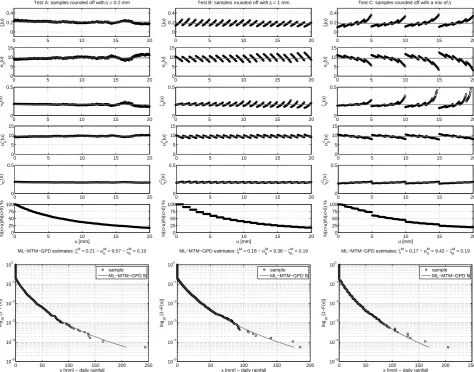
Fig. 6. Same as Fig. 4, but here the MTM is applied on three synthetic samples generated by Eq. (10) and discretized according to the
rounding rules of test A (0.2 mm resolution), B (1 mm resolution), and C (mixing of resolutions up to 5 mm): results of each test are shown in columns from left to right, respectively. The sixth row of subplots now shows the percentage of records exceeding each thresholduwith respect to the number of strictly positive records.
Examples of MTM application on 50-yr synthetic time se-ries generated by Eq. (10) with parametersξ=0.2,α0=9 mm,
andζ0=0.2 are shown in Fig. 6: each column reports the
re-sults for a sample extracted from one the groups of tests A, B, and C. As in previous Figs. 2 and 4, the first three rows of subplots show the unconditioned estimates ofξ,α0, andζ0
as a function of the threshold, while the fourth and fifth rows show the reduction of the spread for conditioned estimates α0C, andζ0C, but again the signature of the roundings is still visible. Comparing these results with those in the previous Fig. 4, we can observe a strong similarity with the patterns obtained for historical daily rainfall time series. Moreover, in the first column of subplots of Fig. 6 (time series discretized with 0.2 mm resolution) we can again observe the increasing dispersion of the unconditioned estimates ofξ,α0, andζ0for
thresholds larger than the MTM range. As already discussed for Fig. 2, this dispersion can be related to the increasing
estimation variance as the number of excesses decreases. It is worth noticing on the second and third columns of subplots of Fig. 6 how the increasing dispersion is hidden by the ef-fects of roundings. Finally, the last row of subplots in Fig. 6 shows a comparison between the empirical survival functions and Eq. (10) parameterized withξM,α0M, andζ0MMTM es-timates: again we can visually appreciate the good results of the proposed approach and the reliable fitting to the highest quantiles.
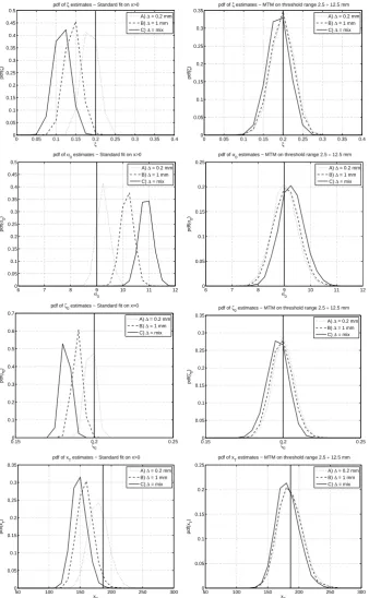
Figure 7 shows the relative frequency distributions of ξ, α0,ζ0, andx50estimates provided by the standard fit (left
col-umn) and the MTM fit (right colcol-umn) on 5000 Monte Carlo samples discretized according to tests A, B, and C. The ver-tical lines in each subplot show the parameter values used for generations (ξ=0.2,α0=9 mm, andζ0=0.2) and the
ex-pected 50-yr return period quantilex50=187 mm. A visual
[image:10.595.59.534.64.436.2]0 0.05 0.1 0.15 0.2 0.25 0.3 0.35 0.4 0
0.05 0.1 0.15 0.2 0.25 0.3 0.35 0.4 0.45 0.5
pdf of ξ estimates − Standard fit on x>0
ξ
pdf(
ξ
)
A) Δ = 0.2 mm
B) Δ = 1 mm
C) Δ = mix
0 0.05 0.1 0.15 0.2 0.25 0.3 0.35 0.4
0 0.05 0.1 0.15 0.2 0.25 0.3 0.35
pdf of ξ estimates − MTM on threshold range 2.5 ÷ 12.5 mm
ξ
pdf(
ξ
)
A) Δ = 0.2 mm
B) Δ = 1 mm
C) Δ = mix
6 7 8 9 10 11 12
0 0.05 0.1 0.15 0.2 0.25 0.3 0.35 0.4 0.45 0.5
pdf of α0 estimates − Standard fit on x>0
α0
pdf(
α0
)
A) Δ = 0.2 mm
B) Δ = 1 mm
C) Δ = mix
6 7 8 9 10 11 12
0 0.05 0.1 0.15 0.2 0.25
pdf of α0 estimates − MTM on threshold range 2.5 ÷ 12.5 mm
α0
pdf(
α0
)
A) Δ = 0.2 mm
B) Δ = 1 mm
C) Δ = mix
0.150 0.2 0.25
0.1 0.2 0.3 0.4 0.5 0.6 0.7
pdf of ζ0 estimates − Standard fit on x>0
ζ0
pdf(
ζ0
)
A) Δ = 0.2 mm
B) Δ = 1 mm
C) Δ = mix
0.150 0.2 0.25
0.05 0.1 0.15 0.2 0.25 0.3 0.35
pdf of ζ0 estimates − MTM on threshold range 2.5 ÷ 12.5 mm
ζ0
pdf(
ζ0
)
A) Δ = 0.2 mm
B) Δ = 1 mm
C) Δ = mix
50 100 150 200 250 300
0 0.05 0.1 0.15 0.2 0.25 0.3 0.35
pdf of x
T estimates − Standard fit on x>0
xT
pdf(x
T
)
A) Δ = 0.2 mm
B) Δ = 1 mm
C) Δ = mix
50 100 150 200 250 300
0 0.05 0.1 0.15 0.2 0.25
pdf of x
T estimates − MTM on threshold range 2.5 ÷ 12.5 mm
xT
pdf(x
T
)
A) Δ = 0.2 mm
B) Δ = 1 mm
[image:11.595.130.469.74.623.2]C) Δ = mix
Fig. 7. Relative frequency distributions ofξ, α0 andζ0and corresponding 50-yr quantiles on 5000 GPD random samples discretized
according to test A (resolution1=0.2 mm, dotted lines), B (1=1 mm, dashed lines), and C (mixing of resolutions up to1=5 mm, solid lines). Results from the standard fit method with a single thresholdu=0 (all strictly positive records are used) and from the MTM applied in a range of thresholds between 2.5 mm and 12.5 mm are shown in the left and right column, respectively. From top to bottom, the plots display results forξ,α,ζ0and 50-yr quantile estimates. Vertical thick solid lines show the parameters of Eq. (10) used for Monte Carlo
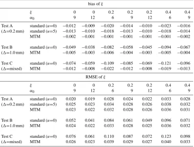
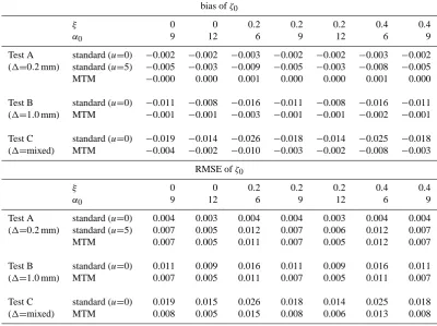
Table 1. Bias (top part of the table) and RMSE (bottom part) of MLξestimates obtained by the standard fit with a single thresholdu=0 and the MTM fit on a range of thresholds between 2.5 to 12.5 mm. Parameters are estimated from synthetic samples generated by Eq. (10) with different couples of shapeξand scaleα0GPD parameters andζ0=0.2. Each sample is 50-yr long and is discretized according to test A
(0.2 mm resolution), B (1 mm resolution), and C (mixing of resolutions up to 5 mm). For test A, results for the standard fit with a single thresholdu=5 mm are also presented.
bias ofξ
ξ 0 0 0.2 0.2 0.2 0.4 0.4
α0 9 12 6 9 12 6 9
Test A standard (u=0) −0.012 −0.009 −0.020 −0.014 −0.010 −0.023 −0.016 (1=0.2 mm) standard (u=5) −0.013 −0.010 −0.018 −0.013 −0.010 −0.018 −0.014 MTM −0.002 −0.001 −0.001 −0.001 −0.001 −0.001 −0.002 Test B standard (u=0) −0.049 −0.038 −0.082 −0.058 −0.045 −0.094 −0.067 (1=1.0 mm) MTM −0.005 −0.003 −0.006 −0.004 −0.003 −0.005 −0.004 Test C standard (u=0) −0.074 −0.059 −0.109 −0.085 −0.069 −0.121 −0.096 (1=mixed) MTM −0.012 −0.008 −0.022 −0.012 −0.008 −0.019 −0.013
RMSE ofξ
ξ 0 0 0.2 0.2 0.2 0.4 0.4
α0 9 12 6 9 12 6 9
Test A standard (u=0) 0.020 0.019 0.028 0.024 0.022 0.033 0.028 (1=0.2 mm) standard (u=5) 0.025 0.023 0.034 0.028 0.026 0.038 0.032 MTM 0.023 0.022 0.032 0.028 0.026 0.036 0.031 Test B standard (u=0) 0.052 0.041 0.084 0.061 0.049 0.096 0.071 (1=1.0 mm) MTM 0.024 0.022 0.033 0.028 0.025 0.036 0.032 Test C standard (u=0) 0.076 0.061 0.110 0.087 0.072 0.123 0.098 (1=mixed) MTM 0.026 0.023 0.039 0.029 0.027 0.040 0.033
a clear picture of the bias affecting the standard fit estimates: the larger the discretization, the higher the bias. On the other hand, looking at the corresponding subplots in the right col-umn we can observe how the MTM is not affected by these bias problems: the only visible drawback is a slight increase of the estimation variance related to the lower number of ex-ceedances used for MTM estimations.
Figures presented and discussed till now give us a qualita-tive but quite clear idea of MTM supremacy on the standard fit. Nevertheless, in order to provide an objective evalua-tion of the MTM performances, we evaluated bias and RMSE of the two fitting approaches for each group of rounding-off tests and GPD parameters:
biasθˆ = Ehθˆ −θi RMSEθˆ =
s
E
ˆ θ −θ2
(12)
where θˆ is an estimator (provided by the standard or the MTM approach) of the parameterθ. In our case the θ pa-rameter can beξ,α0,ζ0, or the 50-yr return period quantile
x50. For each parameter, results in term of bias and RMSE
are presented in Tables 1, 2, 3, and 4, respectively. We do not show results in terms of estimation variance, since it can be easily obtained as var(θ )ˆ =RMSE(θ )ˆ 2−bias(θ )ˆ 2. But we
would like to highlight that the estimation variance of the standard fit (on all strictly positive records) is expected to be lower than the one of the MTM fit, since var(θ )ˆ of ML esti-mators is asymptotically inversely proportional to the sample size: as shown in the sixth row of subplots in Fig. 6, the num-ber of exceedances of the MTM range of thresholds varies between about 75% and 25% of all strictly positive records.
An overall look at the tables clearly reveals how perfor-mances can drastically change depending on the resolution of the sample (test A, B, and C) and also on the shape and scale parameter values. However some general behaviours can be identified.
The top part of each table shows the bias for each param-eter: we can observe a clear supremacy of the MTM against the standard fit for all the considered discretizations and for all the couples (ξ,α0) of GPD parameters. The qualitative
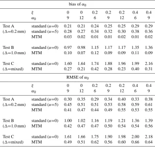
Table 2. Same as Table 1 but forα0estimates.
bias ofα0
ξ 0 0 0.2 0.2 0.2 0.4 0.4
α0 9 12 6 9 12 6 9
Test A standard (u=0) 0.21 0.21 0.24 0.25 0.25 0.29 0.29 (1=0.2 mm) standard (u=5) 0.28 0.27 0.34 0.32 0.30 0.38 0.36 MTM 0.03 0.02 0.01 0.01 0.02 0.01 0.02 Test B standard (u=0) 0.97 0.98 1.15 1.17 1.17 1.35 1.36 (1=1.0 mm) MTM 0.10 0.07 0.12 0.09 0.09 0.11 0.09 Test C standard (u=0) 1.60 1.64 1.74 1.88 1.96 1.99 2.16 (1=mixed) MTM 0.27 0.21 0.42 0.28 0.23 0.40 0.31
RMSE ofα0
ξ 0 0 0.2 0.2 0.2 0.4 0.4
α0 9 12 6 9 12 6 9
Test A standard (u=0) 0.30 0.35 0.29 0.34 0.40 0.33 0.38 (1=0.2 mm) standard (u=5) 0.45 0.51 0.51 0.53 0.58 0.59 0.61 MTM 0.41 0.47 0.44 0.49 0.55 0.53 0.55 Test B standard (u=0) 1.00 1.02 1.16 1.19 1.21 1.36 1.39 (1=1.0 mm) MTM 0.42 0.47 0.47 0.50 0.54 0.54 0.56 Test C standard (u=0) 1.61 1.66 1.75 1.90 1.98 2.00 2.18 (1=mixed) MTM 0.49 0.51 0.62 0.56 0.60 0.66 0.64
for the other couples of GDP parameters: the MTM is able to correct most of the bias affecting the standard fit.
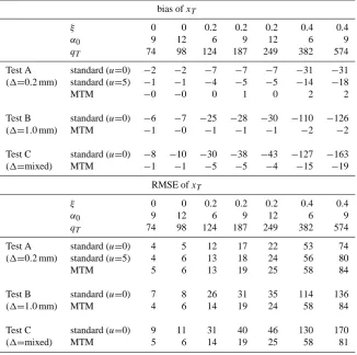
The bottom part of the tables reports the evaluation of per-formances in term of RMSE. We can still observe a clear supremacy of the MTM for samples discretized according to test B and C. For test B, where samples are rounded off at a 1 mm resolution, the RMSE for the standard fit is about 2– 3 times larger than the one for the MTM fit, while for test C (roundings up to 5 mm) the ratio of RMSEs of the two fitting approaches increases to about 3–4. Thus there is no doubt about the advantage of applying the MTM approach on sam-ples with records rounded off at 1 mm or higher resolutions. Moreover, it is worthwhile noticing that in the case of test C, where 30% of records were rounded off at a 5 mm resolution, the RMSE of the standard fit assumes unacceptable values if compared to the range of GPD parameters estimated on our database (Fig. 5): e.g. the RMSE(ξ) is of order 0.1 while the range of estimates in our database is between 0 and 0.4, simi-lar arguments hold also forα0since RMSE(α0)≈2 mm while
α0estimates range from 6 to 12 mm.
Now, let us draw some considerations on the RMSE for test A, where all records were discretized at a resolution 0.2 mm. Although this is the standard resolution of most tipping-bucket rain gauges in Europe, results for this test can
Table 3. Same as Table 1 but forζ0estimates.
bias ofζ0
ξ 0 0 0.2 0.2 0.2 0.4 0.4
α0 9 12 6 9 12 6 9
Test A standard (u=0) −0.002 −0.002 −0.003 −0.002 −0.002 −0.003 −0.002 (1=0.2 mm) standard (u=5) −0.005 −0.003 −0.009 −0.005 −0.003 −0.008 −0.005 MTM −0.000 0.000 0.001 0.000 0.000 0.001 0.000 Test B standard (u=0) −0.011 −0.008 −0.016 −0.011 −0.008 −0.016 −0.011 (1=1.0 mm) MTM −0.001 −0.001 −0.003 −0.001 −0.001 −0.002 −0.001 Test C standard (u=0) −0.019 −0.014 −0.026 −0.018 −0.014 −0.025 −0.018 (1=mixed) MTM −0.004 −0.002 −0.010 −0.003 −0.002 −0.008 −0.003
RMSE ofζ0
ξ 0 0 0.2 0.2 0.2 0.4 0.4
α0 9 12 6 9 12 6 9
Test A standard (u=0) 0.004 0.003 0.004 0.004 0.003 0.004 0.004 (1=0.2 mm) standard (u=5) 0.007 0.005 0.012 0.007 0.006 0.012 0.007 MTM 0.007 0.005 0.011 0.007 0.005 0.012 0.007 Test B standard (u=0) 0.011 0.009 0.016 0.011 0.009 0.016 0.011 (1=1.0 mm) MTM 0.007 0.005 0.011 0.007 0.005 0.011 0.007 Test C standard (u=0) 0.019 0.015 0.026 0.018 0.014 0.025 0.018 (1=mixed) MTM 0.008 0.005 0.015 0.008 0.006 0.013 0.008
In the light of these results we strongly suggest the use of the MTM not only on roughly rounded-off data, but also on correctly discretized records as in test A for the following reasons. Firstly, when we increase the threshold to a reliable valueu∗for the standard fit, the RMSEs become the same for the two approaches, but the MTM does not suffer from bias problems. Secondly, RMSE of MTM is acceptable anyway if compared to the range of GPD parameters values estimated on our database (Fig. 5). Thirdly, the MTM does not require an exact determination of the optimum threshold, but a vi-sual analysis like we made in our dataset can suffice: the median value on the wide range of thresholds is robust even in the case that a small number of estimates are obtained on thresholds smaller than the optimum one u∗ for each ana-lyzed station; on the other hand, applying the standard fit on the excesses of a wrong thresholdu<u∗will certainly lead to a higher bias and consequently a higher RMSE (see e.g. the estimates for thresholds lower than 3 mm in Fig. 2).
6 Final remarks and conclusions
Special caution should always be taken when representing the distribution of rainfall records collected at a daily or any other fixed time scale by dealing separately with the zero and non zero records and by fitting any distribution function on all strictly positive records: indeed the smallest values usu-ally depart from the distribution of the bulk of the records and can introduce a bias in the parameter estimates (as shown in Fig. 2). Thus, whatever distribution is candidate to describe daily rainfall, we need to choose a proper threshold to reli-ably describe our sample by the fitted distribution.
Theoretical arguments suggest modelling threshold ex-ceedances by the generalized Pareto distribution (GPD), moreover empirical evidences support this choice for rain-fall records. Thus derivations and applications presented in this paper are focused on the GPD, but many concepts are quite general and applicable to other distributions.
Table 4. Same as Table 1 but forx50extreme quantile estimates corresponding to a 50-yr return period.
bias ofxT
ξ 0 0 0.2 0.2 0.2 0.4 0.4
α0 9 12 6 9 12 6 9
qT 74 98 124 187 249 382 574
Test A standard (u=0) −2 −2 −7 −7 −7 −31 −31 (1=0.2 mm) standard (u=5) −1 −1 −4 −5 −5 −14 −18
MTM −0 −0 0 1 0 2 2
Test B standard (u=0) −6 −7 −25 −28 −30 −110 −126 (1=1.0 mm) MTM −1 −0 −1 −1 −1 −2 −2 Test C standard (u=0) −8 −10 −30 −38 −43 −127 −163 (1=mixed) MTM −1 −1 −5 −5 −4 −15 −19
RMSE ofxT
ξ 0 0 0.2 0.2 0.2 0.4 0.4
α0 9 12 6 9 12 6 9
qT 74 98 124 187 249 382 574
Test A standard (u=0) 4 5 12 17 22 53 74 (1=0.2 mm) standard (u=5) 4 6 13 18 24 56 80
MTM 5 6 13 19 25 58 84
Test B standard (u=0) 7 8 26 31 35 114 136 (1=1.0 mm) MTM 4 6 14 19 24 58 84 Test C standard (u=0) 9 11 31 40 46 130 170 (1=mixed) MTM 5 6 14 19 25 58 81
selecting only those time series that were discretized at a 0.2 mm resolution, we found a stabilization of the shape pa-rameter for thresholds larger than 3–4 mm. Thus, we as-sumed an optimum threshold located around these values. Nevertheless, should other values be more reliable in other regions, the methods proposed here can be applied anyhow on revised ranges of thresholds.
The GPD is usually fitted on rainfall time series (or other hydrological variables) through the following steps: (i) iden-tification of a single optimum threshold u∗ for each time series with any numerical or graphical method; (ii) estima-tion of the probability of threshold excesses, e.g. counting the number of exceedances; (iii) inference of GPD shape and scale parameters on the exceedances over the selected optimum threshold with any parameter estimator. In order to represent and reproduce a time series, or to estimate ex-treme quantiles, four parameters for each site should be de-termined: the shapeξ and scaleαu∗parameters of the fitted GPD, the thresholdu∗and the probabilityζ
u∗to observe ex-ceedances over the threshold. Nevertheless,αu∗andζu∗ es-timates are not the best indicators of climatological spatial patterns, because of their dependence on the thresholdu∗.
In this paper we provided equations to eliminate this de-pendence of parameters on the threshold and to describe the rainfall distribution with the simple representation in Eq. (10), where only the three threshold-invariant parame-tersξ,α0, andζ0 are used. In such a way, even if we are
analyzing different stations where we observe a good fit-ting of exceedances distributions with different values of the thresholds, once the fitting has been completed we can forget the threshold values, and use Eq. (10) without any explicit parameter dependence on the thresholds. This is a desired property for regional analyses since the three parametersξ, α0, andζ0reflect only the climatic signature.
Using this threshold-invariance property of the ξ, α0,
and ζ0 parameters we developed the Multiple Threshold
Method (MTM) which provides the three estimates as the median values of reparameterizations over a proper range of thresholds. We have also shown how the MTM is par-ticularly able to filter out the deviations from threshold-invariance which are artificially driven by the presence of roughly rounded-off records. Indeed, despite the fact that ξ, α0, and ζ0 reparameterizations are expected to be
expected values, but the median operator is robust even in case of asymmetric fluctuations of the estimates, as found on historical time series with roughly rounded-off records and on synthetic samples discretized at different resolutions. The range of thresholds adopted here for the MTM is between 2.5 and 12.5 mm: in our opinion this is the best trade-off be-tween the need to have a range wide enough to filter out fluc-tuations artificially driven by the roundings, but also small enough to have an acceptable estimation variance, and finally we are quite confident that most of the thresholds are larger than the optimum one, at least in the database analyzed here. However, as already remarked, if there is evidence of dif-ferent optimum threshold values in other regions, the MTM range of thresholds can be consequently revised.
The Monte Carlo method was systematically applied to evaluate and compare the performances of the MTM against the single-threshold standard fit in terms of bias and RMSE, considering different discretizations, as well as different shape and scale GPD parameters. Results of our analysis clearly prove the supremacy of the MTM with respect to the standard fit in case of roughly rounded-off records, while in the test devised for records discretized at a 0.2 mm resolution (like most EU tipping-bucket rain gauges) the RMSE for the MTM resulted about the same as the standard fit with a sin-gle threshold around u=5 mm, but MTM has the smallest bias. Thus in conclusion the MTM always performs better than the standard single-threshold fit regardless of the record discretizations. Moreover, we strongly recommend the MTM also because the results provided by the median operator over a wide range of thresholds should not be affected by small er-rors in the location of the optimum threshold, as conversely happens for the single-threshold standard fit.
All the analyses were performed with the ML, nevertheless the MTM can be applied anyhow on the estimates provided by any other estimator.
Acknowledgements. This research was funded by the Fulbright
Program. The author gratefully acknowledges the comments and suggestions made by Giuseppe Mascaro and Michelangelo Puliga, and the in-depth review by Andreas Langousis.
Edited by: A. Cancelliere
References
Balkema, A. A. and de Haan, L.: Residual lifetime at great age, Ann. Probab., 2, 792–804, 1974.
Beguer´ıa, S.: Uncertainties in partial duration series modelling of extremes related to the choice of the threshold value, J. Hydrol., 303, 215–230, 2005.
Beguer´ıa, S., Vicente-Serrano, S. M., L´opez-Moreno, J. I., and Garc´ıa-Ruiz, J. M.: Annual and seasonal mapping of peak in-tensity, magnitude and duration of extreme precipitation events across a climatic gradient, northeast Spain, Int. J. Climatol., 29, 1759–1779, doi:10.1002/joc.1808, 2009.
Cameron, D., Beven, K., and Tawn, J.: An evaluation of three stochastic rainfall models, J. Hydrol., 228, 130–149, 2000. Castillo, E.: Extreme values theory in engineering, Academic Press,
San Diego, 1988.
Cheng, M. and Qi, Y.: Frontal Rainfall-Rate Distribution and Some Conclusions on the Threshold Method, J. Appl. Meteorol., 41, 1128–1139, 2002.
Cho, H. K., Bowman, K. P., and North, G. R.: A Comparison of Gamma and Lognormal Distributions for Characterizing Satel-lite Rain Rates from the Tropical Rainfall Measuring Mission, J. Appl. Meteorol., 43, 1586–1597, 2004.
Choulakian, V. and Stephens, M. A.: Goodness-of-Fit Tests for the Generalized Pareto Distribution, Technometrics, 43, 478–484, 2001.
Coles, S.: An introduction to statistical modeling of extreme values, Springer-Verlag, London, 2001.
Coles, S. and Dixon, M.: Likelihood-Based Inference for Extreme Value Models, Extremes, 2, 5–23, 1999.
Coles, S., Pericchi, L. R., and Sisson, S.: A fully probabilistic approach to extreme rainfall modeling, J. Hydrol., 273, 35–50, 2003.
Cunnane, C.: A particular comparison of annual maxima and partial duration series methods of flood frequency prediction, J. Hydrol., 18, 257–271, 1973.
Davison, A. C. and Smith, R. L.: Models for exceedances over high thresholds, J. Roy. Stat. Soc. B Met., 52, 393–442, 1990. De Michele, C. and Salvadori, G.: Some hydrological applications
of small sample estimators of Generalized Pareto and Extreme Value distributions, J. Hydrol., 301, 37–53, 2005.
Deidda, R.: An efficient rounding-off rule estimator: Application to daily rainfall time series, Water Resour. Res., 43, W12405, doi:10.1029/2006WR005409, 2007.
Deidda, R. and Puliga, M.: Sensitivity of Goodness of Fit statistics to rainfall data rounding off, Phys. Chem. Earth, 31, 1240–1251, doi:10.1016/j.pce.2006.04.041, 2006.
Deidda, R. and Puliga, M.: Performances of some parameter esti-mators of the generalized Pareto distribution over rounded-off samples, Phys. Chem. Earth, 34, 626–634, doi:10.1016/j.pce. 2008.12.002, 2009.
Dupuis, D. J.: Exceedances over high thresholds: A guide to thresh-old selection, Extremes, 1, 251–261, 1998.
Fisher, R. A. and Tippett, L. H.: Limiting forms of the frequency distribution of the largest or smallest member of a sample, in: Mathematical Proceedings of the Cambridge Philosophical So-ciety, 24, 180–190, doi:10.1017/S0305004100015681, 1928. Fitzgerald, D. L.: Single station and regional analysis of daily
rain-fall extremes, Stoch. Hydrol. Hydraul., 3, 281–292, 1989. Gnedenko, B. V.: Sur la distribution limite du terme maximum
d’une s´erie al´eatoire, Ann. Math., 44, 423–453, 1943.
Grimshaw, S. D.: Computing Maximum Likelihood Estimates for the Generalized Pareto Distribution, Technometrics, 35, 185– 191, 1993.
Guillou, A. and Hall, P.: A Diagnostic for Selecting the Threshold in Extreme Value Analysis, J. Roy. Stat. Soc. B Met., 63, 293– 305, 2001.