www.hydrol-earth-syst-sci.net/16/3165/2012/ doi:10.5194/hess-16-3165-2012
© Author(s) 2012. CC Attribution 3.0 License.
Earth System
Sciences
A novel approach to analysing the regimes of temporary streams
in relation to their controls on the composition and structure
of aquatic biota
F. Gallart1, N. Prat2, E. M. Garc´ıa-Roger2,*, J. Latron1, M. Rieradevall2, P. Llorens1, G. G. Barber´a3, D. Brito4, A. M. De Girolamo5, A. Lo Porto5, A. Buffagni6, S. Erba6, R. Neves4, N. P. Nikolaidis7, J. L. Perrin8, E. P. Querner11, J. M. Qui ˜nonero3, M. G. Tournoud8, O. Tzoraki7, N. Skoulikidis9, R. G´omez10, M. M. S´anchez-Montoya10, and J. Froebrich11
1IDAEA, CSIC, Jordi Girona 18, 08034 Barcelona, Spain 2FEM, D. Ecologia, UB, 08028 Barcelona, Spain
3CEBAS, CSIC, 30100 Murcia, Spain 4IMAR, 3004-517 Coimbra, Portugal 5IRSA, CNR, 70132 Bari, Italy
6IRSA, CNR, 20861 Brugherio MB, Italy 7EED, TUC, 73100 Chania, Greece
8Universit´e Montpellier 2, 34095 Montpellier, France 9HCMR, 19013 Anavissos, Athens, Greece
10Dept. Ecolog´ıa e Hidrolog´ıa, UMU, 30100 Murcia, Spain 11Alterra, 6708 PB, Wageningen, The Netherlands
*present address: ICBIBE, UV, 46980 Paterna, Val`encia, Spain
Correspondence to: F. Gallart ([email protected])
Received: 14 October 2011 – Published in Hydrol. Earth Syst. Sci. Discuss.: 31 October 2011 Revised: 14 August 2012 – Accepted: 14 August 2012 – Published: 6 September 2012
Abstract. Temporary streams are those water courses that undergo the recurrent cessation of flow or the complete dry-ing of their channel. The structure and composition of biolog-ical communities in temporary stream reaches are strongly dependent on the temporal changes of the aquatic habitats determined by the hydrological conditions. Therefore, the structural and functional characteristics of aquatic fauna to assess the ecological quality of a temporary stream reach cannot be used without taking into account the controls im-posed by the hydrological regime. This paper develops meth-ods for analysing temporary streams’ aquatic regimes, based on the definition of six aquatic states that summarize the transient sets of mesohabitats occurring on a given reach at a particular moment, depending on the hydrological condi-tions: Hyperrheic, Eurheic, Oligorheic, Arheic, Hyporheic and Edaphic. When the hydrological conditions lead to a change in the aquatic state, the structure and composition of
determine the presence of different biotic assemblages. This novel concept links hydrological and ecological conditions in a unique way. All these methods were implemented with data from eight temporary streams around the Mediterranean within the MIRAGE project. Their application was a precon-dition to assessing the ecological quality of these streams.
1 Introduction
Temporary streams are water courses whose flow regime is characterized by the recurrent interruption of flow or even the complete drying of their channel. This type of water course is not only widespread in dry climate areas (e.g. Rossouw et al., 2005; Levick et al., 2008), but also constitutes the first-order stream network in many drainage basins in wetter climates (Fritz et al., 2006). The frequency of these streams is ex-pected to increase in the near future because of both climate warming and rising water consumption due to human activ-ities (Tooth, 2000; Larned et al., 2010). The interruption of the aquatic conditions in temporary streams plays a determi-nant role in their ecological communities (Boulton, 1989; Ar-scott et al., 2010), so much so that temporary streams should be considered a distinct class of ecosystems instead of sim-ply hydrologically challenged permanent streams (Larned et al., 2010). Indeed, the traditional perception among man-agers that a “healthy” stream must flow all year round can no longer be sustained (Boulton et al., 2000), though there are still severe gaps in our knowledge of these streams that affect their sound management.
As extreme states, large floods are considered to be short but important disturbance events on aquatic biota, as they imply an indiscriminate “washing” effect of most species (Boulton and Lake, 1992; pulse disturbances in Lake, 2003). Only the most resilient and resistant species are found just after a major flood event. This diminishes ecological qual-ity metrics if sampling is done soon after a flood. In the reverse situation, no aquatic invertebrates – except in re-sistant forms (e.g. cysts, cocoons, diapausing eggs) – are present when there is no surface water (Boulton, 1989). Even when only disconnected pools are present, biotic commu-nities are not representative of the actual ecological status of the stream, since conditions may vary among and within pools over time, even under reference conditions. These de-pend on many factors (e.g. pool size, pool water temperature and quality, stochastic assemblage of refugees, etc.) (Boul-ton, 1989; Buffagni, et al., 2009; press disturbance in Lake, 2003). Only when flow is present (in either the Eurheic or Oligorheic states defined below) are the diversity of habitats and the environmental conditions sufficient to sustain a bio-logical aquatic community representative of biobio-logical qual-ity. The current metrics used to establish ecological status in permanent streams can only be applied in these two cases (e.g. Munn´e and Prat, 2009, 2011).
Many hydrological and ecological studies, using diverse metrics, have been devoted to the hydrological characteriza-tion of temporary streams. The frequency of zero-flow peri-ods (or its complement, flow permanence) is the first crite-rion for most of them (e.g. Hedman and Osterkamp, 1982; Poff, 1996). The seasonality of these periods is also used in some classifications (Uys and O’Keeffe, 1997; Rossouw et al., 2005; Kennard et al., 2010). A few authors also take into account the occurrence of isolated pools during periods with-out flow (Uys and O’Keeffe, 1997; Boulton et al., 2000). In fact, in ecological terms, the more relevant characteristics of the water regime in temporary streams are not flow values, but the temporal and spatial patterns of occurrence or disap-pearance of the features of the aquatic habitats that depend on the presence and flow of water (hereafter called meso-habitats sensu Salo, 1990), such as riffles and pools as well as the connectivity of water flow between them (e.g. Lake, 2007; Bonada et al., 2007; Chaves et al., 2008). While the information recorded at network gauging stations consists of water discharges, the occurrence of the diverse habitats and particularly of pools above and below the station during peri-ods of zero discharge is not recorded, despite their prominent ecological role (e.g. Uys and O’Keeffe, 1997; Bond and Cot-tingham, 2008).
increases. This has been highlighted recently by Sheldon et al. (2010); in their Fig. 3 they depicted how the assemblage of organisms in a long-lasting disconnected pool is dominated by generalist species with lower diversity, a conclusion simi-lar to the results found formerly in Bonada et al. (2007). For this reason the ecological status of the streams should not be measured during the disconnected pools phase.
How biological metrics defining ES using macroinverte-brates may change from wet to dry periods was investigated recently by Munn´e and Prat (2011), who showed that in dry periods in Mediterranean streams there is always less rich-ness than in wet years, although in another study (Rose et al., 2008) the comparison of spring samples when riffles are present gave similar values between years despite the hydro-logical conditions of the year (dry or wet).
In temporary streams, only when the hydrological controls on aquatic life are completely understood, the impact of hu-man changes on biota and the ES can be appropriately as-sessed. For fish studies, pools should remain the entire year round if they are intended to be used for biomonitoring (not necessarily for macroinvertebrates and algae) and it is clear that the fish community would be very dependent on the changes of water quality of pools over time (Magalh¨aes et al., 2007; Benejam et al., 2010; Dewson et al., 2007; see also the review of Williams, 2006). In these cases (based on fish studies), the dependence of fish characteristics on the water quality of pools is clear. Thus, for temporary rivers, before the evaluation of the biological condition of streams for cal-culating ES, hydrological conditions (and their influence on mesohabitat composition) should be studied.
In this context, the present study puts forward a composite approach for analysing the hydrological conditions of tem-porary streams on the basis of their controls of the occur-rence of aquatic mesohabitats relevant to the development of aquatic life at the reach scale. This approach is designed for both research and management purposes and consists of four closely-related aspects:
The first aspect consists of the characterisation of the di-verse states of a stream aquatic system when the hydrologi-cal conditions change. Boulton (2003) outlined the existence of “critical stages” in macroinvertebrate aquatic systems, de-fined by critical thresholds of discharge or water level at which mesohabitats become isolated or dry during a drought. Later on, Fritz et al. (2006), in an outstanding field manual, defined five hydrologic conditions that describe the diverse levels of connectivity or fragmentation of the aquatic phase in headwater streams from “no surface water” (0) to “surface flow continuous” (4). Here, the concept of aquatic state (AS) is introduced; it summarizes the set of aquatic mesohabitats occurring on a given reach at a particular moment, depending on the hydrological conditions. Six ASs are defined: Hyper-rheic, EuHyper-rheic, OligoHyper-rheic, AHyper-rheic, Hyporheic and Edaphic (definitions provided below). The AS concept is consistent with the two earlier definitions and the relationships between them are analysed below along with their definition. The set
of aquatic mesohabitats that occurs on a temporary stream reach is known to be crucial for the presence and abun-dance of aquatic fauna. Pools act as refuges for fish, provid-ing places of survival durprovid-ing the absence of flow (Magoulick and Kobza, 2003) or influencing their vigour (Spranza and Stanley, 2000), while riffles are necessary for filter-feeder organisms that need the current for their nourishment. The effect of the mesohabitat conditions on the community of macroinvertebrates has been studied in some detail (Fem-inella, 1996; Bonada et al., 2006; Acu˜na et al., 2005), as well as the interactions between different trophic levels (Lundlam and Magoulick, 2009). Comparing communities before and following multi-year droughts (Magalh¨aes et al., 2007) or the comparison between communities in temporary and perma-nent streams (Rieradevall et al., 1999; Mas-Mart´ı et al., 2010) emphasized the importance of knowing both the present AS and its evolution over time. It is known that fauna in tempo-rary streams are more complex and taxa richness may even be higher than in permanent ones; the replacement of differ-ent ASs through the year gives opportunities to a succession of species typical of riffles and then of ponds, making their final richness greater than in many permanent streams (e.g. Bonada et al., 2006; Garc´ıa-Roger et al., 2011; Punt´ı et al., 2007). The EPT index (Number of taxa of Ephemeroptera, Plecoptera and Trichoptera) and EPT versus OCH (Taxa of Odonata, Coleoptera and Heteroptera) are good indicators of changes in mesohabitat conditions (Bonada et al., 2006). The importance of mesohabitats and the heterogeneity they give the river (microhabitat conditions) has been highlighted re-cently in temporary streams by Garc´ıa-Roger et al. (2011, 2012).
which shows the annual variation in the occurrence of the di-verse aquatic states. These graphic methods enable the tem-poral patterns of occurrence of the ASs of a temporary stream to be seen quickly, but do not allow the quantitative assess-ment of the stream regime that is necessary versus biological metrics and for comparisons between stream reaches.
Therefore, the third aspect of the approach develops some metrics for the efficient characterisation, ranking and com-parison of stream regimes, as well as for analysing the re-lationships with biological indices or metrics. In the present study, only metrics focusing on the analysis of the statistics of zero flow were considered, as cessation of flow is the only flow discharge feature directly linked to some major change in the ASs available from flow records, and it may be con-sidered the key feature defining the aquatic regime in a tem-porary stream (Boulton, 1989). Indeed, although many stud-ies are devoted to characterizing the flow regime of streams for ecological or management purposes with diverse metrics, most of these metrics are conceived for permanent flow. For example, the Richards-Baker flashiness index (Baker et al., 2004) assigns zero flashiness values during the periods with-out flow because there is no change in the discharge values within them; subsequently but inconsistently, the longer the annual period without flow in a stream, the lower the flashi-ness index is.
The fourth and last aspect addresses a classification of the aquatic regimes (ARs) of temporary streams, based on the existing ones. The AR refers here to the long-term aggre-gated temporal schedule of flow and no-flow periods, which characterizes the general hydrological conditions of a stream, but only indirectly its mesohabitat or microhabitat condi-tions. There is some agreement on the main terminology used for classifying temporary stream regimes, but the cri-teria used to establish the limits between the classes vary be-tween different authors (Uys and O’Keeffe, 1997; Boulton et al., 2000; Rossouw et al., 2005; Levick et al., 2008). We pro-pose a conceptual classification that tries to summarize the main types of temporal hydrological discontinuities relevant to the occurrence of aquatic mesohabitats, paying less atten-tion to the limits between the types. Nevertheless, to be op-erational, this classification needs to be applicable to streams using recorded or modelled hydrological data. For this pur-pose, the use of the metrics developed in the former aspect for classifying stream ARs is attempted.
Overall, this approach is intended to be used for three main purposes: (i) improved investigation of the hydrolog-ical restrictions on the development of aquatic life; (ii) the characterisation and classification of aquatic stream meso-habitat conditions (aquatic states), which helps managers to define the ES of streams; and (iii) the design of biologi-cal sampling biologi-calendars (i.e. scheduling biota sampling at the more ecologically significant moments: see Bond and Cot-tingham, 2008). The ultimate goal is the development of tools for characterising the hydrological controls on the develop-ment of aquatic life in stream reaches for both research and
management applications. In fact, this method is being devel-oped within the European MIRAGE project, which addresses the improvement of the WFD by regulating the inclusion of temporary streams.
2 Methodological approach
The approach developed consists of four steps, two on the definition and analysis of the ASs and two on the ARs, as in-troduced above. Though the data necessary for determining ASs and ARs are the same, they use different approaches and metrics. In the first step, the ASs, establishing the mesohabi-tat conditions relevant to the growth of aquatic life in tempo-rary streams, are defined. In the second step, the flow thresh-olds between ASs are assessed using field observations and the flow duration curve, allowing us to investigate the tem-poral patterns of occurrence for the 5 wetter ASs at the reach scale, using hydrographs and the ASFG. In the third step, as the periods with zero flow are the key identifiable hydrolog-ical driver of biologhydrolog-ical communities, the metrics that best characterize the frequency and predictability of these periods are developed and analysed. Finally, the fourth step consists of the updated classification of the ARs of temporary streams and its implementation using the metrics developed. The first and second steps are sequential; the third and fourth steps can follow in any order.
The data used here for implementing the AS and AR meth-ods come from the records from gauging stations at several sites around the European Mediterranean (Fig. 1). Table 1 shows the location and main hydrological characteristics of these sites. These gauging stations are located on streams with discharges that are not influenced by human activities, or only slightly, except for the V`ene S station where sum-mer flows are sustained by effluents from urban sewage sys-tems (David et al., 2011). The Vallcebre and V`ene streams are research basins where flow data were directly recorded by the teams involved in the MIRAGE project (Latron and Gallart, 2008; Perrin and Tournoud, 2009), whereas the flow data from the other stations were obtained from the respec-tive basin authorities.
The time scale used through the different steps is the month, although a daily scale was used for analysing the his-tory of the AS during the months before the sampling cam-paigns. The monthly scale was selected for long-term analy-ses because it is easier to manage and to obtain from records or models and it is usually sufficient for the development of the aquatic fauna. A finer temporal scale would result in too spiky data, because short occasional events would not be pooled unless the series lasted for many years.
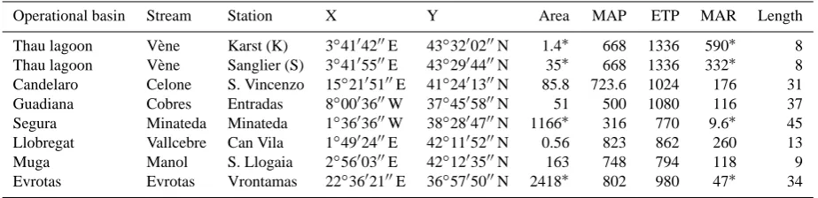
Table 1. Main characteristics of the studied basins. Catchment area in km2; MAP = mean annual precipitation (mm); ETP = mean annual reference evapotranspiration (mm); MAR = mean annual runoff (mm), Length = available record length in years.
Operational basin Stream Station X Y Area MAP ETP MAR Length Thau lagoon V`ene Karst (K) 3◦4104200E 43◦3200200N 1.4∗ 668 1336 590∗ 8 Thau lagoon V`ene Sanglier (S) 3◦4105500E 43◦2904400N 35∗ 668 1336 332∗ 8 Candelaro Celone S. Vincenzo 15◦2105100E 41◦2401300N 85.8 723.6 1024 176 31 Guadiana Cobres Entradas 8◦0003600W 37◦4505800N 51 500 1080 116 37 Segura Minateda Minateda 1◦3603600W 38◦2804700N 1166∗ 316 770 9.6∗ 45 Llobregat Vallcebre Can Vila 1◦4902400E 42◦1105200N 0.56 823 862 260 13 Muga Manol S. Llogaia 2◦5600300E 42◦1203500N 163 748 794 118 9 Evrotas Evrotas Vrontamas 22◦3602100E 36◦5705000N 2418∗ 802 980 47∗ 34
∗karstic areas with uncertain real groundwater recharge area.
zCandelaro
zVène
zEvrotas
zManol
zEnxoé zMinateda
zVallcebre
Fig. 1. Location of the main streams studied.
field observations or the simulations made with a model de-signed for this purpose (e.g. Arscott et al., 2010).
2.1 Defining the ecologically relevant aquatic states (AS)
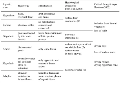
The ASs summarize the transient sets of aquatic mesohabi-tats occurring on a given stream reach at a particular moment, depending on the hydrological conditions. From a review of the literature (Hawkins et al., 1993; Gasith and Resh, 1999; Boulton, 2003; Fritz et al., 2006; Lake, 2007) and the ex-pertise of some of the authors (e.g. Rieradevall et al., 1999; Bonada et al., 2006, 2007; Garc´ıa-Roger et al., 2011), the following ASs may be defined as relevant in the ecology of temporary stream reaches, in a sequence from wetter to drier (see Table 2). The terms were selected in a way similar to the widely accepted grades in aquatic ecology for nutrient avail-ability (i.e. Eutrophic, Mesotrophic, Oligotrophic) or pollu-tion (i.e. Oligosaprobic, Mesosaprobic) that grade from the highest (hyper-) to the lowest condition (A-, Hypo-), using here the Greek suffix “-rheos” as indicating flowing water:
– Hyperrheic: infrequently high water (flood) causes ma-jor movement of stream bed alluvium and the drift of most of the aquatic fauna in the reach. In permanent streams, this state corresponds to flow above bankfull discharge, but temporary streams may not show dis-tinct channel banks. Observations of temporary streams
suggest that floods cause a strong but short-lived dis-turbance (pulse disdis-turbances in Lake, 2003) in aquatic communities (Boulton and Lake, 1992; Lake, 2000; Ar-scott et al., 2010), whereas their occurrence is consid-ered highly relevant to the health of river systems (Junk et al., 1989). In low gradient rivers of dry areas, over-bank floods may be the periods of the highest biological productivity due to the release of nutrients from sedi-ments and detritus in the alluvial plain (e.g. Walker et al., 1995). This state is not differentiated from the fol-lowing one in the schemes of both Fritz et al. (2006) and Boulton (2003).
– Eurheic: water discharge is high enough to allow the occurrence of all the available aquatic habitats in the reach, including the abundant presence of riffles, and to allow optimum hydraulic connectivity between the di-verse habitats. This is the habitual state in permanent streams and the one with the widest range of discharges in temporary streams; a succession of riffles and pools (macrohabitats) is the rule, with great variability in mi-crohabitat conditions (Garc´ıa-Roger et al., 2012). This state corresponds to the “surface flow continuous (4)” condition defined by Fritz et al. (2006), whereas Boul-ton (2003) differentiated two intermediate states above or below the critical step of the water body’s “isolation from the littoral vegetation”, suggesting the existence of a subsequent state that we could call Mesorheic. Nev-ertheless, we decided not to use this intermediate state here because, as already mentioned by this author, the associated loss of species is rather low and it might be relevant only for certain particular conditions, such as large rivers or wetlands in low-gradient areas.
[image:5.595.49.287.244.346.2]step of “loss of riffle”. When few riffles persist, the riffle macroinvertebrate community can be still effective for bio-monitoring, but it tends to resemble that of pools and edges, due to decreased flow and increased lentic habitats (e.g. Bonada et al., 2006; Rose et al., 2008). – Arheic: surface discharge is null or close to zero, but
a number of water pools remain in the stream bed. If this is alluvial, some sub-surface connectivity of wa-ter may occur, allowing the preservation of the physico-chemical quality of the water in the pools for some time at least. If the stream bed is impervious, the pool wa-ters are vulnerable to undergoing quality deterioration trends or cycles. The ecological importance of pools re-maining after the cessation of flow has been highlighted in many papers (e.g. Boulton, 1989), but when the connection lasts for many weeks, the pools tend to dis-appear (through evaporation) and water quality may de-teriorate rapidly. In large dryland rivers, persistent pools (usually named waterholes in Australia) play a primary role in river ecology as refugia of many species dur-ing the long periods between flow events (Sheldon et al., 2010). This state corresponds to both “surface water present but no visible flow (2)” and “surface water in pools only (1)” conditions defined by Fritz et al. (2006), whereas it is just mentioned but not differentiated in a critical step from the former state in Boulton (2003). – Hyporheic: most of the stream bed is devoid of surface
water in the reach, although alluvium may remain wet enough to allow hyporheic life (alluvium water content is higher than the field capacity point). Only terrestrial fauna may be observed on the surface of the stream bed, but since the hyporheic zone may be a refuge for many animals when surface water is absent (Boulton, 1989; Boulton et al., 1998), it should also be considered an aquatic mesohabitat. This state is included within the “no surface water (0)” condition defined by Fritz et al. (2006), and below the “loss of surface water” critical step defined by Boulton (2003).
– Edaphic: the entire stream bed is devoid of surface wa-ter in the reach and alluvium is dry enough to impede active hyporheic life (alluvium water content is lower than field capacity and similar to the surrounding soils in terrestrial locations). The active life in the alluvium is similar to the edaphic life in the interfluvial soils, but some invertebrates may survive in desiccation-resistant stages in dry substrata for some time (Boulton, 1989). This state is also included within the “no surface water (0)” condition of Fritz et al. (2006), and mentioned as “drying hyporheic zone” but not separated from the for-mer state by any critical step by Boulton (2003). Only terrestrial fauna exist on the surface and, if the state lasts for many weeks, the river bed may be invaded by terres-trial plants, creating a quite different ecosystem.
Most of these adjectives are already in use: Hyperrheic, Oligorheic and Arheic illustrate regional water drainage lev-els, so there is no possible confusion with the terms defined in this work. Hyporheic designs the ground zone below the stream bed saturated with some proportion of water coming from the stream and Edaphic is an adjective used for soil life and overall properties and processes; we used the same terms for the ASs when these environments are dominant, making it easier to understand them.
2.2 Time patterns of occurrence of aquatic states
Although temperature and electrical conductivity of either water or bed sediments may be used for recording the tim-ing of hydrological conditions in the absence of flow (Con-stantz et al., 2001; Blasch et al., 2003; Fritz et al., 2006), the only information currently available on stream water regimes is from flow discharge records, coming from either measure-ments at gauging stations or simulations using rainfall-runoff models. Flow records at gauging stations are the most com-monly obtained ones and are usually managed on a daily basis, but the monthly time scale is also commonly used to obtain estimates of flows from climatic data, particularly in scarce data conditions.
Flow data from a gauging station may be used to obtain the statistics of the occurrence of the wetter ASs (Hyper-rheic, Eu(Hyper-rheic, Oligorheic) following the procedure shown in Fig. 2, for which the ASFG.xls spreadsheet is available in the Supplement to assist readers. Alternatively, flow simula-tions obtained with a rainfall-runoff model may be used, but as most models cannot simulate zero water discharges, the identification of a discharge threshold equivalent to zero will be necessary. Once flow thresholds between the AS were as-sessed (as in Fig. 3), we used both daily values, to analyse the regime during a sampling season (Fig. 4), and monthly values to analyse long-term seasonal patterns of occurrence of ASs (Fig. 5).
The most demanding step in the procedure shown in Fig. 2 is the selection of the threshold flow values that separate the occurrence of the various ASs. This can be done with the help of the shape of the flow duration curve (distribution function of flow discharges, Fig. 3). To identify these thresholds cor-rectly, field observations on the ASs synchronous with dis-charge measurements are needed. However, in the absence of these observations, thresholds can be provisionally calcu-lated by taking into account the width and regularity of the stream bed reach near the gauging station. The limitations of this method will be analysed in the Discussion section.
Table 2. Characterisation of the aquatic states in terms of hydrological and ecological features and comparison with two former schemes.
Aquatic Hydrological Critical drought steps state Hydrology Mesohabitats conditions Boulton (2003)
Fritz et al. (2006)
Hyperrheic flood, drift of bedload
surface flow overbank flow and fauna
continuous (4) all mesohabitats
isolation from littoral Eurheic abundant riffles available and
vegetation connected
loss of riffle pools connected lentic fauna with most
flow only Oligorheic by thin water of lotic species
interstitial (3) threads present
surface water present but
drying pool Arheic disconnected only lentic fauna not visible flow (2)
pools surface water
loss of surface water in pools only (1)
no surface water
only hyporheic and
Hyporheic but alluvium terrestrial fauna drying refuges close to
active
no surface water (0)
drying hyporheic zone saturation
alluvium terrestrial fauna and Edaphic moisture as some resistant phases
in interfluves of aquatic fauna
Gauging station flow data
Model flow simulations
Flow thresholds
selection
zero flow threshold
Flow duration curve
Field observations
Aquatic states occurrence
tables months
years
0/1 Flow table months
years
Aquatic states frequency graph
Fig. 2. Schematic flow chart for the procedure developed to estimate
the temporal patterns of occurrence of the aquatic states from the available water flow data. The final products are the ASFGs (Fig. 4).
over impervious bedrock or alluvial ones with gauging sta-tions allowing the bypass of sub-surface flow, minimum recorded flow may be expected to represent the threshold be-tween Arheic and Oligorheic states. Consequently, discharge data cannot be used to derive information on the occurrence of the Edaphic AS in the first case and of the Hyporheic and Edaphic ASs in the second. Once the discharge thresholds between ASs are defined, they are used to convert the table of monthly discharges into the tables of occurrence of these ASs.
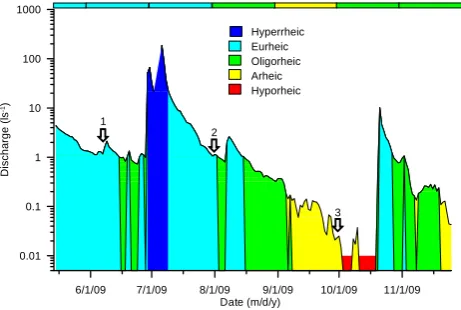
[image:7.595.51.292.125.649.2]When a biological sampling campaign of a stream reach was designed for determination of the ES (see Sect. 2.5 be-low) and the subsequent results were to be analysed in com-parison with the stream regime, the occurrence of the diverse ASs was calculated for the days before and during the sam-pling campaign. The flow hydrograph and the respective ASs corresponding to the sampling campaign held in 2009 at Can Vila (Vallcebre), using a daily temporal unit, is shown in Fig. 4. Note that the arrows indicate the dates when the sam-pling was done.
0 0.2 0.4 0.6 0.8 1
Exceedance frequency
1E-006 1E-005 0.0001 0.001 0.01 0.1
Me
an
mo
nt
h
ly
f
low
(m
3 s
-1
)
arheic oligorheic eurheic
[image:8.595.312.543.63.218.2]hyperrheic
Fig. 3. Flow duration curve for the Vallcebre stream at Can Vila
station, with identification of the minimum discharge thresholds that separate the diverse aquatic states.
the various study sites. The discharge threshold values be-tween ASs were assessed whenever possible with some field observations, using the expertise of the authors, and mini-mum measured flows were taken as the threshold between Hyporheic and Arheic states in the interim.
2.3 Metrics for characterizing the aquatic regime in temporary rivers
The ASFG method given above allows appraisal of the AR of the reach, as it describes the mean annual prevalence and timing of ASs for a stream reach by month. Nevertheless, the information shown is too complex to be synthesised in a few metrics and it depends on the somewhat subjective se-lection of flow thresholds. To circumvent these limitations, it may be hypothesized that the cessation of flow is the key fea-ture defining the AR in a temporary stream (Boulton, 1989) and, therefore, the statistics of its metrics will summarize the main characteristics of the regimes of its ASs, as seen in its ASFG. Therefore, we selected the metrics that synthesize the two main hydrological parameters that are relevant to river ecology: the duration and predictability of periods with and without flow.
The relative time with or without water flow is usually the metric used for identifying temporary streams (e.g. Hedman and Osterkamp, 1982; Hewlett, 1982). Among regional flow regime studies, Poff (1996), in a widely used approach, em-ployed only the mean number of days with zero flow per year; Kennard et al. (2010) used both the mean and the co-efficient of variation of the number of days with zero flow per year, although there are no studies analysing the ecolog-ical significance of this latter metric. In an ecologecolog-ical study of a single stream in New Zealand, Arscott et al. (2010) char-acterised the aquatic regime at several points by using flow permanence (long-term annual average of the percentage of time a given site had flowing water), flow duration (days of flow at a site prior to each sample date) and drying frequency
0.01 0.1 1 10 100 1000
Disc
ha
rge
(
ls
-1)
6/1/09 7/1/09 8/1/09 9/1/09 10/1/09 11/1/09
Date (m/d/y) Hyperrheic Eurheic Oligorheic Arheic Hyporheic
1
2
[image:8.595.51.285.63.209.2]3
Fig. 4. Hydrograph and aquatic states during the 2010 biological
sampling campaign at Vallcebre, Can Vila.
(average number of drying transitions per year). Arscott’s re-sults showed that flow permanence and duration correlated closely, with the former being well related to ecological fea-tures (see also Larned et al., 2010).
From these studies, it can be concluded that two metrics deserve to be retained for further investigation here: a mea-surement of flow permanence (a concept less ambiguous than flow duration), as the long-term mean annual relative number of months with flow, Mf (taking values between 0 and 1), and the drying frequency, Df, as in Arscott et al. (2010).
Besides these flow permanence and drying frequency met-rics, several authors point to the relevant ecological role of the predictability of wetting or drying periods, because this predictability allows the development of taxa special-ized in living in temporary conditions (e.g. Williams, 2006; Wissinger et al., 2008). As no suitable specific metrics were found in the literature, the predictability of the zero-flow pe-riods was analysed using theP,CandMpredictability met-rics of Colwell (1974), and a new measurement, seasonality of drying (Sd6), was developed below.
Colwell (1974), on the basis of Shannon’s entropy, defined three metrics adequate for analysing the periodicity of the qualitative states of a system. These metrics were first de-fined on the basis of monthly system states for analysing sea-sonal periodicity during the year, but other time scales may be used. Following this author, seasonal predictability (P) of the monthly states of a system may be attained by two sepa-rable additional components: constancy (C), a measurement of state permanence, and contingency (M), a measurement of the repeatability of the time pattern in successive years. Here, the two system states considered are zero and positive values of discharge in the records of the gauging stations.
In addition to these metrics, the six-month seasonal pre-dictability of dry periods (Sd6)defined in Eq. (1) is here
Sd6=1− X6
1Fdi/ X6
1Fdj
(1) where Fdi represents the multi-annual frequencies of 0-flow
months for the contiguous 6 wetter months of the year and Fdj represents the multi-annual frequencies of 0-flow
months for the remaining 6 drier months. Wet and dry 6-month periods mean here those with fewer and more zero-flow frequencies, respectively. The calculation of this met-ric is also made easier for the reader through use of the ASFG.xls spreadsheet available in the Supplement.
This variable is dimensionless and takes the value of 0 when zero flows occur equally throughout the year in the long run and 1 when all the zero flows occur in the same 6-month period every year. When the regime is fully perma-nent, this metric cannot be computed, so the value of 1 is set to indicate full predictability. It should be mentioned that Sd6
is defined at the 6-month scale, whereas the Colwell (1974) metrics were applied at the monthly scale. This was done to investigate the full capacity of these metrics, although the potential role of changing temporal scale was tested as stated below.
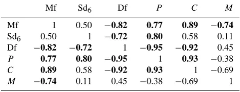
Redundancy between these six metrics (Mf, Sd6, Df,P,C
andM) was analysed by calculating the linear correlation co-efficients when applied to the eight basins studied here (Ta-ble 3). All three of Colwell’s (1974) predictability metrics (P,CandM) correlated significantly with flow permanence (Mf) and the first two correlated negatively with drying fre-quency (Df), whereas Sd6only correlated significantly with
predictability (P). The possible role of the time scale in the use ofP,CandMmetrics was analysed by calculating them on the same 6-month periods used for the Sd6 metric; the
resulting 6-month values had correlation coefficients higher than 0.98 of the monthly values, showing that negligible in-formation was added with this change of scale.
Given the high correlation coefficients between the other metrics, only flow permanence (Mf) and the seasonal pre-dictability of dry periods (Sd6)were selected for the
subse-quent analyses. The former (or its conversion into the number of days with zero-flows) has been widely used and found to be significant for explaining aquatic fauna, whereas the latter is the more orthogonal of the metrics tested and is easy to put into plain words in interviews when information from in-struments is not available. This does not mean that the other metrics tested might not be useful for other analyses or for the investigation of ARs in other types of climate.
2.4 Classifying temporary stream aquatic regimes
[image:9.595.310.545.105.195.2]Although the ASFG and regime metrics shown in the preced-ing sections are fully informative for analyspreced-ing and compar-ing temporary stream regimes, a classification of temporary streams within the perspective of the present paper is nec-essary for operational purposes, as different stream regimes will need different sampling strategies and standards for
Table 3. Linear correlation coefficients between the metrics tested
to analyse the statistics of zero flow periods in the basins studied. Values in bold are significant at thep <0.05 level.
Mf Sd6 Df P C M
Mf 1 0.50 −0.82 0.77 0.89 −0.74
Sd6 0.50 1 −0.72 0.80 0.58 0.11
Df −0.82 −0.72 1 −0.95 −0.92 0.45
P 0.77 0.80 −0.95 1 0.93 −0.38
C 0.89 0.58 −0.92 0.93 1 −0.69
M −0.74 0.11 0.45 −0.38 −0.69 1
defining the biological quality of stream waters (e.g. Bond and Cottingham, 2008), which is one of the most impor-tant objectives of the MIRAGE project. Although there is some agreement on the main terminology for classification of temporary stream regimes, the criteria used to establish the limits between regime classes vary between different au-thors (Rossouw et al., 2005; Levick et al., 2008). On the basis of the above considerations and the classifications proposed by Uys and O’Keeffe (1997) and Boulton et al. (2000), four main conceptual types of streams were defined by the MI-RAGE project in function of the controls imposed by the time patterns of occurrence of aquatic mesohabitats on biological communities and their relevance for monitoring purposes:
– P (permanent or perennial): no relevant recurrent con-trols imposed on biological communities by lack of flow. Monitoring methods have already been defined (e.g. Hering et al., 2006).
– IP (intermittent-pools): stream’s AR allows every year the development of biological communities similar to those in permanent streams, but afterwards the wet sea-son flow is discontinued and only pools with impover-ished communities remain. Ecological quality may be assessed as for permanent streams, though the biolog-ical sampling calendar may need adaptation to the hy-drological regime. Sampling has to be done during the period with the more persistent flow.
– ID (intermittent-dry): streams usually cease to flow and dry out in summer, but in the wet season biological com-munities similar to those of permanent streams can be found, even if these may vary from year to year. Biolog-ical quality assessment needs to be measured with spe-cific biological metrics somewhat different from those of permanent streams and (very important) a calendar adapted to the hydrological regime.
Hyporheic Arheic Oligorheic Eurheic Hyperrheic Hyporheic Arheic Oligorheic Eurheic Hyperrheic
Hyporheic Arheic Oligorheic Eurheic Hyperrheic
Hyporheic Arheic Oligorheic Eurheic Hyperrheic
Hyporheic Arheic Oligorheic Eurheic Hyperrheic Hyporheic Arheic Oligorheic Eurheic Hyperrheic
Hyporheic Arheic Oligorheic Eurheic Hyperrheic
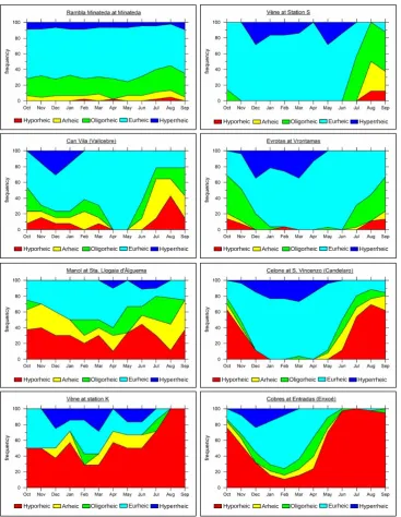
[image:10.595.115.483.61.536.2]Hyporheic Arheic Oligorheic Eurheic Hyperrheic
Fig. 5. Aquatic states frequency graphs for the eight main stream gauging stations in Fig. 1 and Table 1.
study of aquatic fauna (e.g. desiccation-resistant stages of aquatic fauna or terrestrial fauna).
The above classification does not permit any flow statis-tics for defining the boundaries between the classes for two reasons: usually there are no data on the occurrence of pools when flow is zero, and the values of flow statistics may vary between the different regime classes defined, depending on several other variables like temperature regime and charac-teristics of the stream bed. Nevertheless, in order to make the classification usable, we attempted to define the thresh-old values of the hydrological metrics defined in the former
2.5 Measuring the stream’s ecological status
Although the determination of ES is beyond the scope of this paper, some results are given below to show how the approach developed above can be applied.
The ESs of the streams in the MIRAGE project were measured by a standardized protocol (Garc´ıa-Roger et al., 2011, 2012) that provides the same information as the AQEM methodology (Buffagni et al., 2004) and thus the same met-rics for characterizing the ES with which this methodology may be used. As these streams are located in the Mediter-ranean Region, we used metrics designed for these kinds of streams (Munn´e and Prat, 2009). As both are multimetric indices and use the reference condition approach, the EQR value (the ratio between the site value and the value at the reference condition sites) was determined (values close to 1 are good quality; close to 0, bad quality).
The measurement of ecological status (ES) was completed in the MIRAGE streams in 2010 and in Vallcebre in 2009. In each geographical area several sites were studied. If possible, one permanent site was sampled together with an intermittent one during the Arheic state. In both cases, a reference station was selected to check whether there was a disturbed station. This was variable in each basin according to the availabil-ity of the reference/disturbed or the permanent/intermittent stream pairs.
3 Results
3.1 Defining the threshold flow values between aquatic states
Using a few direct observations in the field and the support of the flow duration curve, when available, the interim flow thresholds between ASs were defined for the sites sampled for biological analysis in the MIRAGE project, as shown in Table 4. The thresholds varied according to different river characteristics, especially the size of the basin and the char-acteristics of the stream bed (if it is more or less impervious). Small basins tend to have lower thresholds, which is coher-ent with that, for connecting pools or developing riffles, more flow is needed in a large stream than in a small one. Note also that threshold values were very high in relation to the basin area in one case (V`ene K), which is attributable to this site being a Karstic resurgence whose effective catchment area is much larger than the surface area of the topographic basin. The thresholds for the other stations shown in Fig. 5, not sam-pled for biological analysis, were assessed only from the flow duration curve without field observations.
Of course, differences along the river may be observed in AS occurrence: while upstream the river may be in Eurheic state, downstream it may be in Oligorheic or Arheic states. However, the idea is not to describe in detail the AS of the stream but the conditions at the site that will be sampled for
biological analysis. In the case of MIRAGE data from Ta-ble 4, these were in the vicinity of the gauging stations, be-cause they are relevant for the assemblage of macroinverte-brates that were to be sampled.
3.2 Temporal patterns of occurrence of the aquatic states
Once the water discharge threshold values between the ASs were assessed, the statistics of their occurrence were used for two main purposes: biological sampling design and interpre-tation, and overall regime assessment.
A biological sampling campaign was carried out in 2009 at Can Vila (Vallcebre). Figure 4 shows the hydrograph and the respective ASs during this campaign. Arrows show the bio-logical sampling moments that were scheduled to assess the characteristics of the aquatic macroinvertebrates in the fol-lowing conditions: after a sustained Eurheic state (arrow 1), during an Eurheic state that followed a short Hyperrheic pe-riod (arrow 2), and when pools started to dry out at the end of an Arheic state that followed the same drying sequence (ar-row 3). The methods and results of the sampling of macroin-vertebrate assemblages fall outside the scope of this paper and can be found in Garcia-Roger et al. (2011), which de-scribes them in detail. It is worth emphasizing here that the first sample was discarded for biological analysis and the es-tablishment of ES, because the temperature at this time was low and many of the animals were very small, making identi-fication difficult. Therefore, the second sample was used for further studies. The monitoring of the daily flow of the site made it possible to establish the sampling date in springtime at least two weeks after the last flow peak (four days of Hy-perrheic state by early April, not shown). Also note that the Arheic state period was very late in summer 2009 (Septem-ber), so a sample taken in June would not be representative (in this year) of the dry conditions when only pools remain.
Table 4. Flow thresholds between aquatic states in l s−1defined in different streams studied in different basins of the MIRAGE project.
Stream V`ene V`ene Celone Celone Enxo´e Taibilla Vallcebre Vallcebre Station K S P S Enxo´e Rogativa CV CR Area (km2) 1.4 35 72 24 61 77 0.56 4.17 Hyperrheic >800 >1000 >1000 >200 >100 >1000 >20 >128 Eurheic 100–800 10–1000 30–1000 15–20 10–100 10–1000 1–20 6.4–128 Oligorheic 50–100 3–10 10–30 8–15 1–10 3–10 0.35–1 2.24–6.4 Arheic 10–50 1–3 1–10 1–8 0.1–1 0.05–3 0.05–0.35 0.32–2.24 Hyporheic <10 <1 <1 <1 <0.1 <0.05 <0.05 <0.32
placing the wetter basins at the top and the more seasonal ones on the right-hand side. The ASFG was designed to view the changes of the AS over time and to obtain a first insight into how the sampling calendar should be defined for each basin.
3.3 The aquatic regime of the streams
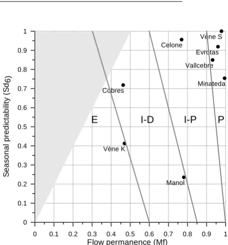
The results obtained with the metrics of flow permanence, Mf, and seasonal predictability of dry periods, Sd6, are
shown in Fig. 6. Here, the stations with the highest flow per-manence are plotted on the right and those with higher sea-sonal predictability at the top. The boundaries between the regime types are tentative, because more sites need to be an-alyzed.
The wetter streams, Rambla Minateda and V`ene at sta-tion S, are both at the outlets of karstic systems and have near-permanent regimes. Nevertheless, the V`ene stream had occasional dry periods in some summers, whereas, in the Rambla de Minateda, dry periods were more scattered throughout the year. Therefore, the respective Sd6 metrics
had different values for these streams and are clearly separate in Fig. 6. The quality of aquatic communities found in these streams should be no different from those living in perennial streams in the region (Permanent type).
At Vallcebre, the regime followed the equinoctial regime of precipitation: flow is more frequent in spring, whereas short-term droughts may be scattered over 9 months of the year. The Evrotas stream showed somewhat higher flow per-manence and a more regular seasonal pattern, with a higher value in the Sd6 metric in Fig. 6. It may be expected that
the aquatic communities in both streams will be similar to those in perennial streams (Permanent type), whereas at Vall-cebre the communities might be expected to be temporar-ily affected by the cessation of flow and eventually by the complete drying of the stream. However, they are expected to be similar to those living in perennial streams if sampled after sufficiently sustained Eurheic states (Intermittent-pools type).
Both the Manol and Celone streams had similar flow per-manence, but the graphs in Fig. 5 show much greater regu-larity for the Celone stream, where continuous flow normally occurs from January to April. Indeed, the Celone stream had
0 0.1 0.2 0.3 0.4 0.5 0.6 0.7 0.8 0.9 1
Flow permanence (Mf)
0 0.1 0.2 0.3 0.4 0.5 0.6 0.7 0.8 0.9 1
S
e
as
on
al
pre
d
ic
tabi
lity
(S
d6)
Manol Vène K
Vène S
Minateda Cobres
Celone
Vallcebre Evrotas
E I-D I-P P
Fig. 6. Plot of the stations studied using the two regime metrics
tested: flow permanence (Mf) and seasonal predictability of the zero-flow months (Sd6). The oblique grey lines show the
approx-imate interim separation between the four regime types: P (Perma-nent), I-P (Intermittent-pools), I-D (Intermittent-dry), E (Episodic-ephemeral). The grey triangle shows a field where the metric values are incompatible.
greater seasonality, as shown by the higher value of the Sd6
metric in Fig. 6. It is worth noting that the features shown for the Manol stream in Fig. 5 and the low Sd6metric are linked
[image:12.595.310.544.184.435.2]Table 5. Frequency of occurrence of aquatic states during the 3 months before the sampling data together with community and biological
water quality metrics for macro-invertebrates at several sites studied in the MIRAGE project. H, E, O, A, Ho = percent time occurrence of the Hyperrheic, Eurheic, Oligorheic, Arheic and Hyporheic states respectively;S= number of taxa; EPT = number of families of Ephemeroptera, Plecoptera and Trichoptera; OCH = Number of families of Odonata, Coleoptera and Heteroptera;H0= Shannon-Wiener diversity Index. IASPT and IMMiT indexes are biological quality indexes expressed in EQR.
Sites H E O A Ho S EPT OCH tax H0 IASPT IMMiT
V`ene K 25 50 0 0 25 4 0 0 0.41 0.11 0.08 V`ene S 25 75 10 0 0 7 0 0 0.84 0.00 0.02 Celone 2 97 0 0 0 39 16 7 1.70 1.21 1.39 Enxo´e 33 17 17 33 0 23 4 5 1.22 0.66 0.75 Vallcebre 0 100 0 0 0 28 10 5 1.67 0.71 0.88 Evrotas 0 100 0 0 0 21 8 5 1.65 0.78 0.81
similar in richness and variety to those in perennial streams (Intermittent-pools type). On the contrary, as aquatic habitats are much less predictable in the Manol stream, aquatic fauna living in this stream are likely to be always less abundant and diverse, yielding low values of the biological metrics due to the hydrological constraints (Intermittent-dry type).
Finally, both the V`ene stream at station K and the Co-bres stream show the lowest frequency of flow occurrence, although the Cobres stream had higher predictability of flow (during winter), as shown in Fig. 5, and a much higher value of the Sd6metric, as shown in Fig. 6. This difference is also
shown here by the drying frequency Df metric, which is as high as 1.63 for the V`ene at station K, but only 0.95 for the Cobres. As in the former example, the characteristics of the aquatic fauna living in these streams are likely to dif-fer because of the large difdif-ference in habitat predictability: the aquatic communities living in the Cobres stream may be well adapted to a dry but predictable regime (Intermittent-dry type), whereas those living in the V`ene K are expected to be rather opportunistic (Ephemeral type).
3.4 Ecological status
The EQR values (the ratio between the site value and value at the reference conditions site) obtained for the ES analy-sis are provided in the two last columns of Table 5 (good quality are values close to 1, bad quality close to 0). Only data for spring are provided here (this was a wet period). As can be seen, we found values of very good (IMMi T-values higher than 0.85) or good (between 0.7 and 0.85) in Cande-laro, Enx¨oe and Vallcebre. As 2010 was a wet year in the Mediterranean area, most of these streams were in Eurheic state at this time. However, data from the V`ene stations show that their ESs were not good (site S) or even very bad (site K). Site S is in a stream reach where, as shown by chemical anal-yses, water quality is highly disturbed because of the spill of effluents from urban waste water-treatment plants (David et al., 2011). Site K is an unimpacted karstic resurgence that was naturally dry for at least 25 % of the time in this pe-riod. Therefore, the poor quality of the EQR value for this stream must be attributed to its AR hindering the presence of
an aquatic macroinvertebrate community similar to those in permanent streams, which is consistent with the location of the V`ene K site on the Fig. 6 graph.
4 Discussion
4.1 Working with aquatic states
The definition of the AS and the use of the ASFG made easier the comparison of the diverse sites studied in the MIRAGE project, the communication among the participants and the design and interpretation of the biological sampling cam-paigns. Nevertheless, we are aware that the main weak point of the method shown above is the possible subjectivity of the determination of the flow thresholds between the ASs.
This is not, however, a particular problem of our approach because the other published approaches that define compara-ble states (Boulton, 2003; Fritz et al., 2006) are similarly sub-jective and much less quantitative when defining the bound-aries between the states or conditions. We went further than these approaches in trying to link qualitative states with flow water measurements, but the relationships between flow dis-charge and ASs are very site-dependent, so exact rules cannot be established. Thresholds are dependent on local conditions for each site and have to be calculated on the basis of local characteristics. Given present methods, ASs are only identi-fiable by field surveys and can only be associated with mea-sured water discharges by direct comparison. Nevertheless, we hope that emerging technologies (e.g. LIDAR, RADAR) will make the remote identification of these transient states in extensive drainage systems possible in the near future.
Aware of these limitations, we used the information on the occurrence of the ASs only as a diagram in the ASFG and decided not to use this information for more quantitative or classification purposes. If a 10-yr flow record is used for building an ASFG, as the resolution of the monthly frequen-cies cannot be greater than 10 %, these statistics cannot be used more rigorously.
or with very few, the ASFG was very informative about the main conditions of the streams and helped set up the sam-pling campaigns. Figure 5 shows clearly that, in a stream like Manol (that may become dry at any month of the year), it is not possible to measure ES using the current methods. On the other hand, in a typical intermittent stream like Celone, the likelihood of finding at least three months of Eurheic state in springtime is very high: thus, evaluation of ES by using the methods suitable for permanent streams is possible.
Along with the visualisation of the ASFGs, the use of flow permanence Mf and seasonal predictability of dry periods Sd6metrics provided a clear and nuanced analysis of the
es-tablishment of ASs and regimes that were relevant for eco-logical assessment and management purposes on the gauged reaches. When more field information is available on the threshold discharges that define the ASs on these reaches, the boundaries between states may be refined in the ASFGs, but their general shape will not change much because they are driven by the statistics of the objective zero flow values.
4.2 Limitations of the graphs and metrics used
The analysis of the ASFG suggests that the duration of the states might be calculated for every month directly from the graph. However, as this graph is a long-term probability anal-ysis, the actual duration (in any given year) must be analysed directly from the data series using other metrics. Here, al-though only the mean annual frequency of drying transitions Df has been tested, other annual or monthly metrics could be used to characterize the statistics of periods with or without flow. Indeed, at the test gauging stations the two metrics on flow permanence and predictability were sufficient to charac-terise and compare the ARs. However, if this kind of analysis is to be applied to temporary streams in other climates, some other metrics may be needed, such as the timing of the drying period if its predictability is high.
This is the case of the Sd6metric, which uses a 6-month
period to analyse the predictability of the period without flow. Because of its definition, its maximum possible values decrease for decreasing values of flow permanence when the latter are lower than 0.5, say less than 6 months of flow (there are no possible values within the upper left signalled area in Fig. 6). Shorter periods might be used for the definition of a similar metric, when streams that normally have less than 6 months of flow are to be analysed.
Another case when other metrics may be necessary is when thermal conditions are another control on aquatic life, superimposed on hydrological controls. The examples used in the present paper come from Mediterranean low- or medium-altitude areas, where the lack of flow is caused by a negative water balance and low temperatures were a marginal limitation for aquatic life (only found at Vallcebre in spring 2009).
4.3 Data availability
Nevertheless, since most temporary streams are ungauged or poorly gauged, the methodology described above will only be applicable to the relatively rare existing records from gauging stations. Rainfall-runoff models were used within the MIRAGE project to obtain simulated flow series for some sites on a monthly scale, but there are two main difficulties even for good performing models: first, most models will not be able to simulate zero water discharges, so the identifica-tion of a discharge threshold equivalent to zero will be neces-sary to use the above-defined metrics (see also Kirkby et al., 2011); and second, simulated values will be natural instead of actual discharges if these are affected by human activi-ties. An exercise on how the metrics change over the years at several sites in the Evrotas basin, depending on the water abstractions, using the SIMGRO model, was performed re-cently (Cazemier et al., 2011). It is a good basis for studying the change of the river’s AR over time and the differences from year to year in the duration of each AS.
Beyond the use of flow data and models, the permanence of flowing water in headwater streams has been operationally calculated from field surveys or topographic map data (Svec et al., 2005; Fritz et al., 2008). The presence of water at the pool scale has also been monitored by using temperature or electrical conductivity observations (Constantz et al., 2001; Blasch et al., 2003; Fritz et al., 2006) or, at the basin scale, remote sensing (Marcus and Fonstad, 2008). It is hoped that emerging technologies (e.g. LIDAR, RADAR) will make possible in the near future the remote identification of some of the ASs in extensive drainage systems, which will help us to understand the differences in the extent of each AS in the basin. However, for the purposes of monitoring ES, knowl-edge of the AS of the site at which the biological sample will be taken is the crucial issue. Of course, detailed knowledge of the AS of the entire basin would give us an idea of the representativeness of such a sample for this basin. The esti-mates of flow permanence obtained through some of these methods might be used to find the zero discharge threshold of a model. Furthermore, the relatively simple meaning of Mf and Sd6metrics may also allow the working classification of
a stream’s AR to be assessed from interviews with people living near the streams, when there are no data available.
Finally, the drier ASs, particularly the Edaphic state, can-not be analysed suitably from flow discharge records or simu-lations. The statistics of these states need other types of data beyond the water discharges usually measured or modelled in scientific or operational hydrology. Nevertheless, the ex-amination of the ASFG may provide some insight into the possibilities of occurrence of these states over the course of the year and, when seasonality is high, it shows when pool occurrence or alluvium moisture needs to be tested for their recognition.
in the stream beds where aquatic communities are replaced by terrestrial communities. But in terms of establishing the ES of the stream, these states are not relevant because no method using terrestrial invertebrates has yet been defined. The MIRAGE project has worked on this topic, but no defini-tive results are available.
4.4 Ecological implications
As the six ASs and the subsequent analyses developed above were designed on the basis of preceding ecological studies in temporary waters, they can be expected to be useful for analysing the controls of the AR in aquatic biological com-munities.
The first results obtained in the European MIRAGE project do indeed suggest this. As shown in the Results sec-tion, all the sites sampled after sustained Eurheic and Olig-orheic states provided biological metrics corresponding to good ES, except the V`ene S site, which is known to be af-fected by water quality deterioration. On the other hand, the V`ene K site, which had shorter Eurheic and Oligorheic states and is known to have a regime that is hard to predict, pro-vided biological metrics corresponding to very bad ES in spite of the good quality of the waters.
Many authors (e.g. Townsend and Riley, 1999) demanded scientific investigation to define if current indices are ro-bust enough with respect to detecting real changes in river health and avoiding the incorrect indication of changes. In this regard, the approach proposed here offers a framework for categorizing river stretches so that biological indices can be more suitably selected and sampling strategies set. This is done by providing an estimation of the AS based on his-torical data, which is assumed to well represent how the ac-tual flow conditions were obtained over time, i.e. accounting for a component of predictability of biological community. This way, a relevant part of overall history behind commu-nity structure is taken into account. On the other hand, the amount and character of habitats actually present at the mo-ment when the sample is taken are crucial also when estab-lishing ES. As far as flow-related habitat assessment is con-cerned, the observed ratio between lentic and lotic in-channel habitats is known to be extremely relevant (Buffagni et al., 2010) and potentially accounts for the most part of commu-nity variance in Mediterranean rivers (Buffagni et al., 2009, 2010). An increase in lentic conditions is often associated with a decrease in metrics used to assess ecological qual-ity, thus possibly causing a serious underestimation of eco-logical quality. Hence, if the presence of lentic conditions is due to natural processes, interannual variation or season, the obtained ES classification can be partly unsubstantiated (Buffagni et al., 2009). In such cases, adaptations or cor-rections to assessment systems are unquestionably needed (Buffagni et al., 2009). Both the quantification of the ac-tual habitat present in the river at the moment of sampling – not under the scope of the present paper – and the definition
of present and antecedent ASs, which provides hydrology-based evidence, should be contemplated in future assessment systems for temporary streams.
The methods described in this paper offer the possibil-ity of extending the biological methods used in permanent streams to the range of temporary stream types if an ade-quate scheduling of the sampling period is made. The recov-ery of the community is highly dependent not only on the duration of the dry period, but also on the predictability of such a period over years. However, if flow is present in the wet period for several months (usually spring), riffles offer the opportunity of measuring biological quality using macro-invertebrates with methods defined for permanent streams (Rose et al., 2008). Nevertheless, the time of sampling must be determined by the hydrological conditions rather than the time of year because, as demonstrated by Munn´e and Prat (2011), wet summers and springs give higher values of metrics than dry springs do. Therefore, the moment when the sample is taken is crucial in establishing ES and should not be linked to a specific time of the year, but to a specific condition of the hydrograph. This was a key issue in the MI-RAGE project and data in Table 5 were collected following this rule. From these data and the work of Rose et al. (2008) and Munn´e and Prat (2009), we can conclude that in tem-porary streams, if samples are taken at the appropriate stage of the hydrograph (after flow has resumed in the stream and been present in it for at least a month), ES may be measured by the same methods as in permanent streams if the values of the Mf and SD6metrics are high enough.
Despite the fluctuations in community assemblages de-scribed in Feminella (1996), Bonada et al. (2006, 2007) and Bˆeche and Resh (2007) and despite the changes from riffle-dominant species (EPT) to pool-riffle-dominant species (OCH), consistency of ES may be measured in both Eurheic (riffle-dominant mesohabitat, but with presence of pools) and Oligorheic (connected-pool mesohabitat conditions) states (Bonada et al., 2007; Rose et al., 2008).
Nevertheless, in streams with low flow permanence Mf and/or low seasonal predictability Sd6, such as the V`ene at K
station, the hydrological controls on biological communities are so high that ecological quality must be measured by either standards specifically designed for them or other alternative methods (e.g. desiccation-resistant stages of aquatic fauna, terrestrial fauna, riparian environment, etc.). These methods are not yet available to managers.
Researchers with data on biological water quality met-rics in temporary streams are invited to test the methods de-scribed above, in order to investigate how temporary stream ARs control aquatic fauna. The ASFG can be prepared and the Mf and Sd6metrics from flow data can be calculated with
Supplementary material related to this article is
available online at: http://www.hydrol-earth-syst-sci.net/ 16/3165/2012/hess-16-3165-2012-supplement.zip.
Acknowledgements. The research leading to these results received
funding from the European Community’s Seventh Framework Programme (FP7/2007-2011) under grant agreement 211732 (MIRAGE project), as well from the Spanish Government under the RespHimed project (CGL2010-18374) and a research contract (Ram´on y Cajal programme) granted to J. Latron. The authors are indebted to M. J. Kirkby, C. Campana, D. von Schiller and V. Andr´eassian for their comments. The editing work of P. Passalacqua and the recommendations of C. Smith and four anonymous reviewers helped to improve the quality of the paper significantly.
Edited by: P. Passalacqua
References
Acu˜na, V., Mu˜noz, I., Giorgi, A., Omella, M., Sabater, F., and Sabater, S.: Drought and postdrought recovery cycles in an inter-mittent Mediterranean stream: structural and functional aspects, J. N. Am. Benthol. Soc., 24. 919–933, 2005.
Arscott, D. B., Larned, S., Scarsbrook, M. R., and Lambert, P.: Aquatic invertebrate community structure along an intermittence gradient: Selwyn River, New Zealand, J. N. Am. Benthol. Soc., 29, 530–545, 2010.
Baker, D. B., Richards, R. P., Loftus, T. T., and Kramer, J.: A new flashiness index: Characteristics and applications to Midwestern rivers and streams, J. Am. Water Resour. As., 40, 503–522, 2004. Bˆeche, L. A. and Resh, V. H.: Short-term climatic trends affect the temporal variability of macroinvertebrate in California Mediter-ranean streams, Freshwater Biol., 52, 2317–2339, 2007. Benejam, L., Angemeier, P. L., Munn´e, A., and Garc´ıa-Berthou,
E.: Assesing effects of water abstraction on fish assemblages in Mediteranean streams, Freshwater Biol., 55, 628–644, 2010. Blasch, K. W., Ferre, T. P. A., Christensen, A. H., and Hoffmann,
J. P.: New field method to determine streamflow timing using electrical resistance sensors, Vadose Zone J., 1, 289–299, 2003. Bonada, N., Rieradevall, M., Prat, N., and Resh, V. H.: Benthic
macroinvertebrate assemblages and macrohabitat connectivity in Mediterranean-climate streams of northern California, J. N. Am. Benthol. Soc., 25, 32–43, 2006.
Bonada, N., Rieradevall, M., and Prat, N.: Macroinvertebrate com-munity structure and biological traits related to flow permanence in Mediterranean river network, Hydrobiologia, 589, 91–106, 2007.
Bond, N. R. and Cottingham, P.: Ecology and hydrol-ogy of temporary streams: implications for sustain-able water management, eWater Technical Report, Can-berra, available at: http://www.ewater.com.au/uploads/files/ Bond Cottingham-2008-Temporary Streams.pdf (last access: 2 September 2012), 2008.
Boulton, A. J.: Over-summering refuges of aquatic macroinverte-brates in two intermittent streams in central Victoria, T. Roy. Soc. South. Aust., 31, 23–34, 1989.
Boulton, A. J.: Parallels and contrasts in the effects of drought on stream macroinvertebrate assemblages, Freshwater Biol., 48, 1173–1185, 2003.
Boulton, A. J. and Lake, P. S.: The ecology of two intermittent streams in Victoria, Australia. III. Temporal changes in faunal composition, Freshwater Biol., 27, 123–138, 1992.
Boulton, A. J., Findlay, S., Marmonier, P., Stanley, E. H., and Valett, H. M.: The functional significance of the hyporheic zone in streams and rivers, Annu. Rev. Ecol. Syst., 29, 59–81, 1998. Boulton, A. J., Sheldon, F., Thoms, M. C., and Stanley, E. H.:
Problems and constraints in managing rivers with variable flow regimes, in: Global perspectives on river conservation: science, policy and practice, edited by: Boon, P. J., Davies, B. R., and Petts, G. E., John Wiley & Sons, London, 415–425, 2000. Buffagni, A., Erba, S., Cazzola, M., and Kemp, J. L.: The AQEM
multimetric system for the southern Italian Apennines: assess-ing the impact of water quality and habitat degradation on pool macroinvertebrates in Mediterranean rivers, Hydrobiologia, 516, 313–329, 2004.
Buffagni, A., Erba, S., Cazzola, M., Murray-Bligh, J., Soszka, H., and Genoni, P.: The Star common metrics approach to the WFD Inter-calibration Process: a full application across Europe for small, lowland rivers, Hydrobiologia, 566, 379–399, 2006. Buffagni, A., Armanini, D. G., and Erba, S.: Does the lentic-lotic
character of rivers affect invertebrate metrics used in the assess-ment of ecological quality?, J. Limnol., 68, 95–109, 2009. Buffagni, A., Erba, S., and Armanini, D. G.: The lentic-lotic
char-acter of Mediterranean rivers and its importance to aquatic inver-tebrate communities, Aquat. Sci., 72, 45–60, 2010.
Capra, H., Pascal, B., and Souchon, Y.: A new tool to interpret mag-nitude and duration of fish habitat variations, Regul. River, 10, 281–289, 1995.
Chaves, M.L., Rieradevall, M., Chainho, P., Costa, J. L., Costa, M. J., and Prat, N.: Macroinvertebrate communities of non-glacial, high altitude intermittent streams, Freshwater Biol., 53, 55–76, 2008.
Cazemier, M. M., Querner, E. P., van Lanen, H. A. J., Gallart, F., Prat, N., Tzoraki, R., and Froebrich, J.: Hydrological analysis of the Evrotas basin, Greece; Low flow characterization and sce-nario analysis, Wageningen, Alterra, Alterra-report 2249, 2011. Colwell, R. K.: Predictability, constancy and contingency of
peri-odic phenomena, Ecology, 55, 1148–1153, 1974.
Constantz, J., Stonestrom, D., Stewart, A. E., Niswonger, R., and Smith, T. R.: Analysis of streambed temperature in ephemeral channels to determine stream flow frequency and duration, Water Resour. Res., 37, 317–328, 2001.
David, A., Perrin, J. L., Rosain, D., Rodier, C., Picot, B., and Tournoud, M. G.: Implication of two in-stream processes in the fate of nutrients discharged by sewage effluents in a temporary river, Environ. Monit. Assess., 181, 491–507, doi:10.1007/s10661-010-1844-2, 2011.