https://doi.org/10.5194/hess-21-3267-2017 © Author(s) 2017. This work is distributed under the Creative Commons Attribution 3.0 License.
Multi-source hydrological soil moisture state
estimation using data fusion optimisation
Lu Zhuo and Dawei Han
WEMRC, Department of Civil Engineering, University of Bristol, Bristol, UK Correspondence to:Lu Zhuo ([email protected])
Received: 13 September 2016 – Discussion started: 14 October 2016 Revised: 17 May 2017 – Accepted: 3 June 2017 – Published: 4 July 2017
Abstract. Reliable estimation of hydrological soil mois-ture state is of critical importance in operational hydrology to improve the flood prediction and hydrological cycle de-scription. Although there have been a number of soil mois-ture products, they cannot be directly used in hydrological modelling. This paper attempts for the first time to build a soil moisture product directly applicable to hydrology us-ing multiple data sources retrieved from SAC-SMA (soil moisture), MODIS (land surface temperature), and SMOS (multi-angle brightness temperatures in H–V polarisations). The simple yet effective local linear regression model is ap-plied for the data fusion purpose in the Pontiac catchment. Four schemes according to temporal availabilities of the data sources are developed, which are pre-assessed and best se-lected by using the well-proven feature selection algorithm gamma test. The hydrological accuracy of the produced soil moisture data is evaluated against the Xinanjiang hydrologi-cal model’s soil moisture deficit simulation. The result shows that a superior performance is obtained from the scheme with the data inputs from all sources (NSE =0.912, r=0.960, RMSE=0.007 m). Additionally, the final daily-available hy-drological soil moisture product significantly increases the Nash–Sutcliffe efficiency by almost 50 % in comparison with the two most popular soil moisture products. The proposed method could be easily applied to other catchments and fields with high confidence. The misconception between the hy-drological soil moisture state variable and the real-world soil moisture content, and the potential to build a global routine hydrological soil moisture product are discussed.
1 Introduction
Soil moisture is a key element in the hydrological cycle, regulating evapotranspiration, precipitation infiltration, and overland flow (Wanders et al., 2014). For hydrological appli-cations, the antecedent wetness condition of a catchment is among the most significant factors for accurate flow gener-ation processes (Berthet et al., 2009; Matgen et al., 2012a). Norbiato et al. (2008) reported that initial wetness conditions are essential for efficient flash flood alerts. Additionally, an operational system requires reliable hydrological soil mois-ture state updates to reduce the time-drift problem (Aubert et al., 2003; Berg and Mulroy, 2006; Dumedah and Coulibaly, 2013). However, currently there is no available soil moisture product that can be used directly in hydrology modelling, pri-marily because soil moisture is difficult to define and there is no single shared meaning in various disciplines (Romano, 2014).
there-fore less applicable to hydrological modelling (Pierdicca et al., 2013); (4) underutilisation of multiple data sources (e.g., multi-angle raw observations by satellite sensors).
Some studies have attempted to directly utilise the ex-isting soil moisture products (i.e., data from satellites, land surface models, and in situ methods directly) for flood pre-diction improvement, for example, Brocca et al. (2010) ex-plored that utilising the soil water index from ASCAT sensor could improve runoff prediction mainly if the initial catch-ment wetness conditions were unknown; Aubert et al. (2003) assimilated in situ soil moisture observations into a sim-ple rainfall–runoff model and acquired better flow prediction performance; Javelle et al. (2010) suggested that estimations of antecedent soil moisture conditions were useful in improv-ing flash flood forecasts at ungauged catchments; contrarily, the Chen et al. (2011) study showed assimilating ground-based soil moisture observations was generally unsuccess-ful in enhancing flow prediction; Matgen et al. (2012b) re-vealed that satellite soil moisture products added little or no extra value for hydrological modelling. Clearly those results are rather mixed. Challenges remain in integrating soil mois-ture estimated outside the hydrological field into hydrologi-cal models. We believe if a hydrologihydrologi-cally directly applicable soil moisture product could be produced, the aforementioned studies’ results would be significantly improved.
Therefore, the aims of this paper are to clarify the afore-mentioned misconception between the hydrological model’s soil moisture state and the real-world soil moisture, assess the data availabilities for direct hydrological soil moisture state estimation, and fuse those available data sources using a hy-drologically relevant approach. It is hoped that the final prod-uct has a superior hydrological compatibility over the exist-ing soil moisture products. To achieve these aims, the Xinan-jiang (XAJ) (Zhao, 1992) operational rainfall–runoff model is used as a target to simulate flow and soil moisture state information (i.e., soil moisture deficit, SMD) for the Pontiac catchment in the central United States (U.S.). The reason for adopting XAJ is explained in the following section. For the purpose of hydrological soil moisture state estimation, it is effective to adopt the data-driven method, which can map multiple data sources into the desired dataset without com-putational burden. In this study the local linear regression (LLR) model is used. The multiple data sources applied in this study include the SMOS (Kerr et al., 2010) multi-angle brightness temperatures (Tbs) with both horizontal (H) and
vertical (V) polarisations, the moderate resolution imaging spectroradiometer (MODIS) (Wan, 2008) land surface tem-perature, and the soil moisture product by SAC-SMA (Xia et al., 2014). The detail explanations of those datasets are cov-ered in the methodology section. A well-proven feature se-lection algorithm gamma test (GT) (Stefánsson et al., 1997; Zhuo et al., 2016b) is employed to pre-assess the selected data inputs and find the optimal combination of them for soil moisture state calculation. In addition, anM-test (Remesan et al., 2008) is adopted to explore the best size of the training
data. The desired soil moisture product is trained and tested by the XAJ SMD simulation. In total four data-input schemes are developed according to the temporal availability of the selected data inputs, which are then combined to give a daily hydrological soil moisture product.
Compared with previous work, our study contains the fol-lowing new elements: (i) a hydrologically directly usable soil moisture product is proposed; (ii) the GT and LLR tech-niques are used for the first time in a data fusion of multiple data sources for hydrological soil moisture state estimation; (iii) the use of multiple data sources is useful, which allows data users to analyse the availability of the different products and compare the relative benefits of them.
2 Material and methods 2.1 Study area
Figure 1.The location and river network of the Pontiac catchment in the U.S., with the flow gauge and NLDAS-2 central grid points (Zhuo et al., 2015a).
The North American Land Data Assimilation System 2 (NLDAS-2) (Mitchell et al., 2004) provides precipitation and potential evapotranspiration information to run the XAJ model. Both data forces are at 0.125◦spatial resolution and
have been converted to daily temporal resolution. In order to use those distributed forcing into the lumped XAJ model, both forcing have been interpolated with the area-weighted average method instead of the more complicated Kriging ap-proach, because the latter could produce errors if not well controlled (Wanders et al., 2014). The average annual rain-fall depth is about 954 mm, and the average annual potential evapotranspiration is approximately 1670 mm. The daily ob-served flow data are acquired from the U.S. Geological Sur-vey.
2.2 Hydrological model
The XAJ hydrological model is used for the simulation of SMD and river flow at a daily time step. It is a simple lumped rainfall–runoff model with many applications performed in world-wide catchments (Chen et al., 2013; Gan et al., 1997; Shi et al., 2011; Zhao, 1992; Zhao and Liu, 1995; Zhuo et al., 2016a, 2015b). Since XAJ can obtain rather effective flow modelling performances and requires only two meteorolog-ical forcing (precipitation and potential evapotranspiration) inputs (Peng et al., 2002), it is used more widely than the more complicated semi-distributed/fully distributed hydro-logical models for operational applications.
As shown in Fig. 2, the XAJ model has three main compo-nents: evapotranspiration, runoff generation, and runoff rout-ing. XAJ consists of soil layers (upper, lower and deep) in its evapotranspiration calculations. Because XAJ adopts the multi-bucket variable-size method in its modelling concept, it has unfixed soil depths, which is more effective than the fixed depths models (Beven, 2012). Other widely used
mod-els such as PDM (Moore, 2007), VIC (Liang et al., 1994), and ARNO (Todini, 1996) also follow this concept.
In XAJ, the three-layer soil moisture state variables are all calculated as SMD, which is an important soil-wetness vari-able in hydrology. SMD is defined as the amount of water to be added to a soil profile to bring it to the field capac-ity (Calder et al., 1983; Rushton et al., 2006). In this study, only the surface SMD (i.e., top layer) referring to the vege-tation and the very thin topsoil, is utilised as a hydrological soil moisture target. This is because the water held in the top few centimetres of the soil has been widely recognised as a key variable associated with water fluxes (Eltahir, 1998; En-tekhabi and Rodriguez-Iturbe, 1994). Moreover, the current satellite technology is only capable of acquiring the Earth in-formation from the outermost layer of the soil. Therefore, as a case study based on the XAJ model, we only focus on the surface soil moisture state investigation here. Future research will focus on the root-zone soil moisture product develop-ment by using a similar method proposed in this study.
Figure 2.Adopted flowchart of the XAJ model (Zhao, 1992). The model consists of an evapotranspiration component(a), a runoff generating component(b), and a runoff routing component(c). P, PET, and ET are the precipitation, potential evapotranspiration, and the simulated actual evapotranspiration respectively; WU, WL and WD represent the upper, lower, and deep soil layers’ areal mean-tension water storage respectively; WM is the areal mean field capacity; EU, EL, and ED stand for the upper, lower, and deep soil layers’ evapotranspiration output respectively; S is the areal mean free water storage; a is the portion of the sub-catchment producing runoff; IMP is the factor of impervious area in a catchment; RB is the direct runoff produced from the small portion of impervious area; R is the total runoff generated from the model with surface runoff (RS), interflow (RI), and groundwater runoff (RG) components respectively. These three runoff components are then transferred into QS, QI, and QG and combined as the total sub-catchment inflow (T) to the channel network. The flow outputs Q from each sub-catchment are then routed to the catchment outlet to produce the final flow result (TQ). The rest of the symbols are explained in Table 1.
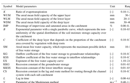
Table 1.The XAJ model parameters used in the Pontiac catchment.
Symbol Model parameters Unit Range
K Ratio of evapotranspiration [–] 0.10–1.20
WUM The areal mean field capacity of the upper layer mm 30–50
WLM The areal mean field capacity of the lower layer mm 20–150
WDM The areal mean field capacity of the deep layer mm 30–400
IMP Percentage of impervious and saturated areas in the catchment % 0.00–0.10 B Exponential parameter with a single parabolic curve, which represents the
non-uniformity of the spatial distribution of the soil moisture storage capacity over the catchment
[–] 0.10–0.90
C Coefficient of the deep layer that depends on the proportion of the catchment area covered by vegetation with deep roots
[–] 0.10–0.70
SM Areal mean free water capacity, which represents the maximum possible deficit of free water storage
mm 10–50
KG Outflow coefficient of the free water storage to groundwater relationships [–] 0.10–0.70 KSS Outflow coefficient of the free water storage to interflow relationships [–] 0.10–0.70
EX Exponent of the free water capacity curve [–] 1.10–2.00
KKG Recession constant of the groundwater storage [–] 0.01–0.99
KKSS Recession constant of the lower interflow storage [–] 0.01–0.99 CS Recession constant in the lag and route method for routing through the channel
system with each sub-catchment
[-] 0.10–0.70
L Lag in time [–] 0.00–6.00
V Parameter of the Muskingum method m s−1 0.40–1.20
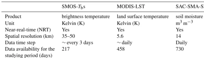
[image:4.612.87.507.447.714.2]Table 2.General data-input properties relevant for this study.
SMOS-Tbs MODIS-LST SAC-SMA-SM
Product brightness temperature land surface temperature soil moisture
Unit Kelvin (K) Kelvin (K) m3m−3
Near-real-time (NRT) Yes Yes Yes
Spatial resolution (km) 35–50 5.6 14
Data time step ∼every 3 days ∼daily Daily
Data availability for the 217 458 730
studying period (days)
obtained larger than 0.80 during both the calibration and val-idation periods. The results are not repeated here.
2.3 Multiple data sources for hydrological soil moisture state estimation
Data sources from SMOS, MODIS, and SAC-SMA are used (Table 2). All data sources have been converted into catchment-scale datasets by the area-weighted average method. The detail description of each data source is given as follows. The main reason for choosing those three data sources is due to their near-real-time (NRT) availabilities (MODAPS Services, 2015; Rodell, 2016) (SMOS becomes available in NRT recently; ESA Earth Online, 2016), which allows for fast implementation in flood forecasting.
2.3.1 SMOS multi-angle brightness temperatures (SMOS-Tbs)
The SMOS (1.4 GHz, L-band) level-3 Tbs data covering
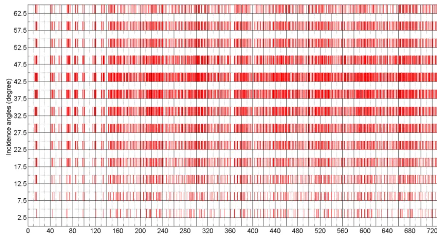
the studying period are available from the Centre Aval de Traitement des Données SMOS (CATDS) (Jacquette et al., 2010). The reason for choosing the SMOS satellite is because compared with other satellite techniques (i.e., optical, and thermal infrared), microwave bands (especially with longer wavelength such as L-band, 21 cm) can penetrate deeper into the soil (∼5 cm) and have less interruptions from weather conditions (Njoku and Kong, 1977). Additionally, SMOS has a relatively longer period of data record compares with other satellite missions such as SMAP. SMOS retrieves the thermal emission from the Earth in both H and V polarisations with wide ranges of incidence angles from 0 to 60◦. The observa-tion depth of SMOS is approximately 5 cm with a spatial res-olution of 35–50 km depending on the incident angle and the deviation from the satellite ground track (Kerr et al., 2012, 2010, 2001).
SMOS providesTbs retrievals at all incidence angles
av-eraged in 5◦width angle bins, which have been transformed into the ground polarisation reference frame (i.e., H, and V polarisations). Therefore, the number of the SMOS-Tbs
in-puts for the hydrological soil moisture estimation can be as high as 24 (12 angle bins per polarisation), with the centre of the first angle bin at 2.5◦in both polarisations
(Rodriguez-Fernandez et al., 2014). As the satellite progresses, any given location on the Earth’s surface is scanned a number of times at various incidence angles, depending on the location with respect to the satellite subtrack: the further away, the fewer the angular acquisitions (Kerr et al., 2010). The data avail-abilities of the SMOS-Tbs are illustrated in Fig. 3 (the
avail-abilities for H and V polarisations are the same). It can be seen that the data availabilities among various incidence an-gles are rather different. In this study the only angle range that gives the most available record of data is from 27.5 to 57.5◦ (i.e., 7 for H and 7 for V polarisation), which is therefore chosen for the hydrological soil moisture develop-ment. This angle range is in line with the angle selection in Rodriguez-Fernandez et al. (2014). In addition the SMOS level-3 soil moisture product from the CATDS (SMOS-SM) is also acquired for a comparison with the estimated soil moisture product. Retrievals that are potentially contami-nated with radio-frequency interference have been removed. Readers are referred to Kerr et al. (2012) for a full de-scription of the SMOS-retrieving algorithms, and Njoku and Entekhabi (1996) for good knowledge of how passive mi-crowaves relate to soil moisture variations.
2.3.2 MODIS land surface temperature (MODIS-LST) The MODIS/Terra (Earth Observing System AM-1 plat-form) (Wan, 2008) daily MOD11C1-V5 land surface tem-perature covering the studied period is downloaded from the Land Processes Distributed Active Archive Centre website. MODIS is chosen among other operational optical satellites for its suitable features, mostly, due to its frequent revisiting time and free NRT data availability. It measures 36 spectral bands between 0.405 and 14.385 µm, and acquires data at three spatial resolutions 250, 500, and 1000 m respectively, while the adopted MOD11C1 V5 product incorporates 0.05◦
com-Figure 3.SMOS-Tbs data availabilities. It is noted that the available dates for the horizontal and the vertical polarisations are the same; therefore, only one is shown here.
pared MOD11C1-V5 land surface temperatures in 47 clear-sky cases with in situ measurement and revealed that the ac-curacy was better than 1 K in the range from−10 to 58◦C in about 39 cases. Cloud-contaminated data have been removed by a double-screening method, and its details can be found in Wan et al. (2002).
2.3.3 SAC-SMA soil moisture estimation (SAC-SMA-SM)
The reason for choosing the SAC-SMA land surface mod-elled soil moisture product is because satellites can often have missing data due to various weather and canopy con-ditions (e.g., rainfall, frozen weather, and vegetation cover-age); therefore, this daily dataset is essential in producing a temporally completed hydrological soil moisture product. In this study, the surface soil moisture (0–10 cm) simulated from the SAC-SMA model is selected. This is because its estimated soil moisture gives a high accuracy against the observational soil moisture and a good correlation with the XAJ SMD (Zhuo et al., 2015b). The daily SAC-SMA-SM is given in a spatial resolution of 0.125◦. The dataset can be download from http://www.emc.ncep.noaa.gov/mmb/nldas/. Readers are referred to Xia et al. (2012) for a full description of the SAC-SMA data products.
2.3.4 Data availabilities
As shown in Table 2, the availability of the three data sources is rather different. Unlike SMOS and MODIS, SAC-SMA-2 SM is a model-based product that runs in a NRT mode, and
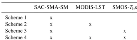
therefore it produces valid data every day during the whole studying period. Whereas the two satellites’ data are more exiguous and depend on weather and surface conditions. Compared with MODIS, the SMOS’s retrieval is even sparse and the biggest data shortage normally occurs in the win-ter season where its returned microwave signal is mostly af-fected by frozen soils (Zhuo et al., 2015a). Based on the data availability analysis, the proposed hydrological soil moisture product is built from four data-input schemes as presented in Table 3. Those four schemes enable us to test and com-pare the estimated soil moisture state more comprehensively. Since the continuity of a soil moisture product is essential for any operational applications, SAC-SMA-SM is included in all of the schemes.
2.4 Data fusion
2.4.1 Gamma test for feature selection
Before model building, it is important to carry out a feature selection process, because it can simplify the model inputs, shorten training times, and reduce overfitting problems. In this study a proper combination of the incidence angles from the SMOSTbs is vital for the best soil moisture state
[image:6.612.74.519.64.304.2]Table 3. Four data-input schemes: scheme 1: SAC-SMA-SM; scheme 2: SM and MODIS-LST; scheme 3: SAC-SMA-SM and SAC-SMA-SMOS-Tbs; scheme 4: SAC-SMA-SM, MODIS-LST, and SMOS-Tbs.
SAC-SMA-SM MODIS-LST SMOS-Tbs
Scheme 1 x
Scheme 2 x x
Scheme 3 x x
Scheme 4 x x x
determines the minimum mean-squared error (MSE) that can be achieved based on the input–output dataset utilising any continuous non-linear models (Zhuo et al., 2016b). The cal-culated minimum MSE is referred to as the gamma statistics and denoted as0. For detailed calculations about the GT al-gorithm, interested readers are referred to Koncar (1997), Pi and Peterson (1994), and Stefánsson et al. (1997). Here only the basic knowledge about the GT is shown:
{(xi, yi) , 1≤i≤M}, (1) where the inputsxi∈Rm are vectors restricted by a closed bounded setC∈Rm, and their corresponding outputsyi∈R are scalars,Mstands for the sample points. The outputsyare determined by the input vectorsxthat carry predictively use-ful messages. The only assumption made is that their latent relationship is from the following function:
y=f (x1. . .xm)+r, (2)
wheref is built up as a smooth model withr representing random noise. Without loss of generality, the assumption of r noise distribution is that its mean is always zero, because all the constant bias has been considered within thef model. Additionally, r’s variance (Var(r))is restricted within a set boundary. The observations’ potential model is now defined within the class of smooth functions.
The 0 is related toN[i, k], which represents as the kth (1≤k≤p) nearest neighbours of each vector xi(1≤i≤ M), written asxN[i,k](1≤k≤p), wherepis a fixed
inte-ger. In order to determine the gamma function from the input vectors, the delta function is used:
δM(k)= 1 M
M X
i=1
xN[i,k]−xi
2
(1≤k≤p), (3)
where the function xN[i,k]−xi
calculates the Euclidean distance. The gamma function for its output values is ex-pressed as in Eq. (4), and the 0 can be determined from Eqs. (3) and (4):
γM(k)= 1 2M
M X
i=1
yN[i,k]−yi
2
(1≤k≤p), (4)
whereyN[i,k]is the corresponding output values for thekth
nearest neighboursxi (xN[i,k]). To find0a least-squared
re-gression line for thep points (δM(k),γM(k)) is built using the following equation:
γ=Aδ+0, (5)
where0can be determined whenδis set as zero. The detailed explanation is
γM(k)→Var(r), when δM(k)→0. (6)
Equation (5) gives us valuable information about the under-lying system; not only that the0is a useful indicator of the optimal MSE result that any smooth functions can achieve, but also its gradientAprovides guidance about the underly-ing model complexity (i.e., the steeper the gradient the more sophisticated the model should be adopted). In this study, the winGamma™ software is used for GT calculation (Durrant, 2001). The mathematical feasibility of GT has been pub-lished in Evans and Jones (2002).
2.4.2 M-test for training data-size selection
A common practice in non-linear modelling is to split the dataset into training and testing parts. However, there is no universal solution on how to divide the datasets (i.e., the pro-portion of each part) so that the best modelling results could be obtained. Here, anM-test is carried out, whereMstands for the training data size.M-test is accomplished by calculat-ing the0for increasing theMvalue (i.e., expanding the train-ing data) and explortrain-ing the resultant graph to judge whether the 0approaches a stable asymptote. Such an approach is straightforward and effective in finding the optimal sizes of training and testing datasets, while avoiding overfitting prob-lems and reducing unsystematic attempts.
2.4.3 Local linear regression
Various data fusion techniques have been developed (Prakash et al., 2012; Srivastava et al., 2013; Wagner et al., 2012); however, their methods require high computational time to run and this, in a real-time flood forecasting framework, could not match the operational needs. Comparatively, the LLR model is a simpler method and requires relatively low computational time. Therefore it is chosen in order to test if a simple method is able to provide effective performance. LLR is a non-parametric regression model that has been applied in Liu et al. (2011), Pinson et al. (2008), Sun et al. (2003), and Zhuo et al. (2016b) for forecasting and smoothing purposes. LLR builds local linear regression based on the nearest points (pmax)of a targeted point, and repeats such a process over the
whole training dataset to produce a piecewise linear model. There are many methodologies in selecting thepmax, in this
Assume there arepmaxnearest points, then Eq. (7) can be
built:
Xm=y, (7)
hereXis apmax×dmatrix, which shows thed-dimensional
information of pmax,xi are the nearest points confined be-tween 1 and pmax,y is the output vector withpmax
dimen-sion, andmis a set of parameters formed in a vector, which plays an important role in mapping the solution fromXtoy. Therefore Eq. (7) can be expanded as
x11 x12 x13 · · · x1d x21 x22 x23 · · · x2d ..
. ... ... . .. ...
xpmax1 xpmax2 xpmax3 · · · xpmaxd
m1 m2 .. . md = y1 y2 .. . ypmax
. (8)
In order to solve the equation, the following two conditions are set: (a) ifXis square and non-singular then Eq. (7) can be simply calculated asm=X−1y; (b) ifXis not square or
sin-gular, Eq. (7) needs to be rearranged andmcan be obtained by finding the minimum of
|Xm−y|2 (9)
with the distinct solution of
m=X#y, (10)
whereX#is the pseudo-inverse matrix ofX(Penrose, 1955, 1956).
3 Results
In this section, different combinations of input data (Table 3) are adopted to examine their impacts on hydrological soil moisture estimation. XAJ SMD is used as a hydrological soil moisture state benchmark for the training and testing. More discussion about the misconception between the hydrolog-ical model’s soil moisture state variable and the real-world soil moisture content is covered in Sect. 4. During GT and M-test processes, all data inputs need to be normalised so that their mean is zero and standard deviation is 0.5. This step is necessary in reducing the impacts of numerical dif-ference from various inputs, hence improving the GT effi-ciency (Remesan et al., 2008). Five statistical indicators are used for the soil moisture estimation analysis: Pearson prod-uct moment correlation coefficient (r), MSE, which is the same value as the gamma statistic 0, standard error (SE), NSE (Nash and Sutcliffe, 1970), and root mean square error (RMSE).
3.1 Scheme 1: SMD estimation using SAC-SMA-SM as input
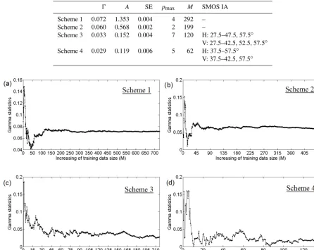
Although in this scheme, there is no need for data feature selection because only one data input is involved, the GT is still carried out to explore the useful information about the underlying relationship between the XAJ SMD and the SAC-SMA-SM. The calculated gamma statistics are shown in Table 4. The0of 0.072 indicates that the optimal MSE achievable using any modelling technique is 0.072; and the small value of SE shows the precision and accuracy of the GT result.0is a significant target value in theM-test to find the most suitable training data size. As presented in Fig. 4a, when more training data (i.e.,M increases in steps of one) is used the0changes dramatically. Eventually atM=292, 0starts to stabilise around 0.072. TheM-test allows us to confidently apply the first 292 datasets to build a model of a given quality, in the sense of predicting with a MSE around the asymptotic level. The corresponding gamma gradient (A) suggests the complexity of the underlying system: the larger theAvalue is the more complex the system is. For example ifAis significantly large, a more complicated model like a support vector machine might be required, butA=1.353 in scheme 1 is small (Remesan et al., 2008); therefore, a LLR model should be able to simulate the system. For LLR mod-elling, its complexity level is controlled by thepmax
param-eter. As illustrated in Fig. 5,pmax is identified from a trial
and error method. The procedure is to increase the LLRpmax
value from 2 to 100 to analyse the variations of their corre-sponding0results. It can be seen from Fig. 5 that the small-est0is achieved atpmax=4, which is therefore adopted for
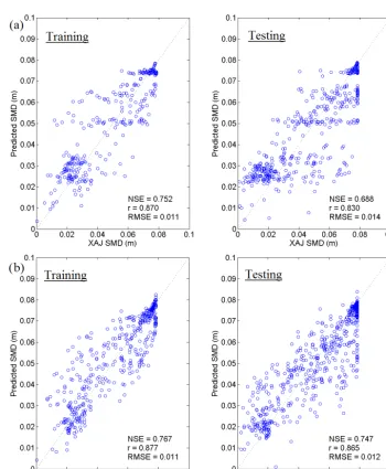
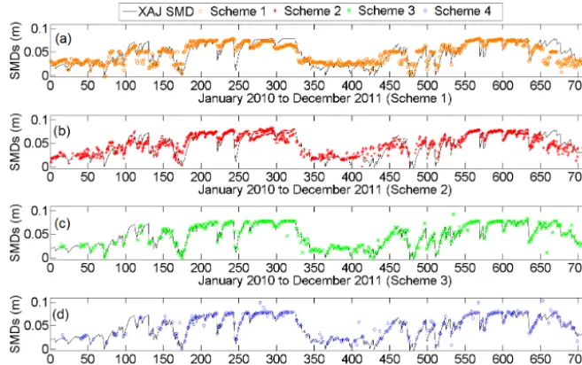
the LLR modelling. The training and testing scatter plots for the LLR modelling are shown in Fig. 6a. It is observed that there are some points lying far above the bisector line during the training period signifying higher estimations, whereas some points sit far below the bisector line during the testing period indicating underestimation of the SMD. For the test-ing results, when XAJ-simulated soil moisture states have al-ready reach the total dryness (i.e., XAJ SMD peaks at around 0.080 m), the predicted soil moisture state is still in the drying process. Figure 7a plots the time series of the estimated and the targeted SMD. The plot shows that the estimated SMD follows the seasonal trend of the soil moisture fluctuations well; therefore, it is wetter during the winter season and exs-iccated during the hot summer season. However, it is clear to see that the model is not able to capture the extreme situations very well, especially during the wet season when the XAJ SMD becomes smaller (e.g., between day 300 and day 350). 3.2 Scheme 2: SMD estimation using SAC-SMA-SM
and MODIS-LST as inputs
Table 4.Model statistical performances and modelling information, where0is the calculated gamma statistic, which is the minimum MSE that can be achieved from a modelling method; Ais the gamma gradient; SE is the Standard error;pmax is the nearest points for LLR modelling;Mis the training data size; and SMOS IA is the chosen incidence angle of SMOS-Tbs.
0 A SE pmax M SMOS IA
Scheme 1 0.072 1.353 0.004 4 292 – Scheme 2 0.060 0.568 0.002 2 199 –
Scheme 3 0.033 0.152 0.004 7 120 H: 27.5–47.5, 57.5◦ V: 27.5–42.5, 52.5, 57.5◦ Scheme 4 0.029 0.119 0.006 5 62 H: 37.5–57.5◦
V: 37.5–42.5, 57.5◦
Figure 4.M-test to find the best training data size:(a)scheme 1,(b)scheme 2,(c)scheme 3, and(d)scheme 4.
(Rodriguez-Fernandez et al., 2015). Therefore, the additional MODIS-LST information could potentially improve the soil moisture estimation. The modelling process is the same as in scheme 1. In Table 4, it is clear to observe that by adding the MODIS-LST input, the0is improved to 0.060 and its corre-sponding gradientAis reduced significantly to less than half of scheme 1. Meanwhile the SE value is decreased remark-ably as well showing the accuracy of the GT. TheM-test in Fig. 4b shows the graph settles to an asymptote around 0.060, which is consistent with the calculated0result. Training data size of 199 is chosen here because it gives the lowest0value. For the LLR modelling, the bestpmaxvalue is found to be 2
from the trial and error result in Fig. 5. The LLR training and testing performances are presented in Fig. 6b. Although the problem of underestimation of extremely dry soil still exists (i.e., the points concentrate at the right end of the training and testing plots), overall the model’s prediction ability during both phases is better than that of scheme 1 (i.e., data points
are closer to the 45◦line). The improvement can also be seen clearly in the time series plot in Fig. 7b. For example, the big disparities between the estimated and the targeted SMDs around day 300 and day 350 are reduced evidently.
3.3 Scheme 3: SMD estimation using SAC-SMA-SM and SMOS-Tbs as inputs
The multi-angleTbs retrievals are the main data inputs for
Figure 5.Gamma statistic (0) variations for increasing the LLRpmaxvalue.
[image:10.612.123.473.278.702.2]Figure 7.The time series plots of the XAJ SMD and the estimated SMD from the four schemes:(a)scheme 1,(b)scheme 2,(c)scheme 3, and(d)scheme 4.
smallest absolute0value. As discussed in Sect. 2.3.4, SAC-SMA-SM is a compulsory data input; therefore, it is not in-cluded in the selecting process. The best set of SMOS-Tbs
to retrieve soil moisture state is composed of H polarisation at the incidence angles of 27.5–47.5, 57.5◦, and V polarisa-tion at the incidence angles of 27.5–42.5, 52.5, 57.5◦. This
result demonstrates that using a combination of H and VTbs
gives a better soil moisture estimation, which is logically sen-sible because different polarisations carry distinct informa-tion of the Earth’s surface. However, some incidence angles could hold common features, which when putting together could result in a negative effect to the LLR modelling, and are therefore not included. The detailed investigation of the possible common features is outside the scope of this paper, which is mainly due to the SMOS working mechanism.
As seen from Table 4, the inclusion of SMOS-Tbs
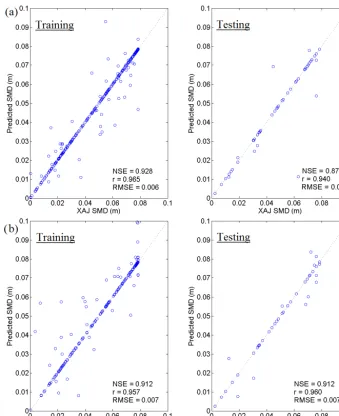
signif-icantly improves the 0 result by 54 %, while the gradient A is reduced greatly by 89 % as compared with scheme 1. The small A value illustrates that the underlying system is more straightforward and easier to model than that of scheme 1. TheM-test analysis in Fig. 4c produces an asymp-totic convergence from a 120 training data size of0 value around 0.033. It is interesting to see that the proportion of the required training data is relatively larger than those in schemes 1 and 2. The potential reason could be explained by the larger amount of data inputs in this scheme. For LLR modelling, thepmaxthat gives the smallest0is 7 (Fig. 5).
The SMD estimations during the training and the testing are presented in Fig. 8a. It can be seen that the SMD prediction ability of this scheme is remarkably better than the previ-ous ones, as most of the points lie on the bisector line al-beit there are still some under- and overestimations. The rea-son SMOS outperforms MODIS in SMD estimation could
be due to the long wavelength the microwave has; therefore, it presents the top few centimetres of the soil while MODIS LST (thermal infrared) only provides information at the soil surface. The used LLR algorithm has been double checked to filter out the potential of an overfitting problem. The check-ing processes are performed by muddlcheck-ing the SMD target in the testing datasets as well as altering the input file, and its efficiency stays the same. Hence, it is believed that the LLR model is very useful in calculating SMD from this scheme. Generally the NSE,rand RMSE statistical indicators show a high agreement during both training and testing phases. For the time series plot in Fig. 7c, it is clear to see that most of the estimated points lie closely to the benchmark line. The observed outliers could be partly due to the data shortage in this scheme so that not all the scenarios are covered in the datasets.
3.4 Scheme 4: SMD estimation using SAC-SMA-SM, MODIS-LST, and SMOS-Tbs as inputs
In this scheme, all the three data sources are used to test if the modelling performance can be further improved. Here the full embedding calculation is again carried out to explore the most suitable incidence angles from the SMOS-Tbs. This
is because the added MODIS-LST data could carry identi-cal (i.e., redundant) features with some of the SMOS-Tbs
datasets. As a result of the full embedding calculation, the best set of SMOS-Tbs is composed of H polarisation at the
vi-Figure 8.LLR modelling during the training and testing phases for(a)scheme 3 and(b)scheme 4.
brates more significantly than the other three schemes, which could be due to the smaller data size and the larger amount of data inputs in this scheme. Here the training data size is chosen as 62 with0obtained at around 0.030. The optimal pmaxis identified to be 5 (Fig. 5). The LLR modelling results
are shown in Figs. 7d and 8b. It is obvious that this scheme further improves the accuracy of the SMD estimation, espe-cially with the high statistical performances achieved during both training and testing phases. Comparatively, this scheme is more stable for SMD estimation, albeit it requires more data inputs and is only realisable when both the MODIS and the SMOS observations are available.
3.5 Produce an unintermitted soil moisture product The data availability of the four schemes varies. As shown in Fig. 9, scheme 1, which has the poorest soil moisture state
[image:12.612.127.467.63.480.2]mois-Figure 9.Data availability plots of the four schemes: scheme 1: SAC-SMA-SM input; scheme 2: SAC-SMA-SM and MODIS-LST inputs; scheme 3: SAC-SMA-SM and SMOS-Tbs inputs; scheme 4: SAC-SMA-SM, MODIS-LST, and SMOS-Tbs inputs. The total available days for the four schemes are 730, 458, 217, and 140 respectively.
Figure 10.Time series plot of the combined daily hydrological soil moisture state estimations.
ture product (Table 5). The time series of the combined soil moisture state is plotted in Fig. 10. It can be seen that the general trend of the produced soil moisture state follows the targeted data very well. However, it tends to overestimate some of the wet events during the rainy season and signif-icantly underestimate the dryer soil condition in September 2011. Those poor estimations are mostly from schemes 1 and 2 where schemes 3 and 4 are not available. Since more and more microwave satellite observations are becoming obtain-able, those new data sources could add extra benefits into the proposed model, and the accuracy of the soil moisture prod-uct is expected to be further enhanced.
4 Discussion
4.1 What is a soil moisture state variable?
This study uses the XAJ’s SMD simulation as a target be-cause it is directly produced by a hydrological model. How-ever, it is argued that models with different parameters values can generate equally good flow results called the equifinality effect, because they are all calibrated based on the observed flow. For this reason, their soil moisture state variables can be distinct among each other.
[image:13.612.126.469.328.513.2]re-Figure 11.SMD variations from the manipulated XAJ calibration (i.e., the WUM parameter is increased by 30 %) and its original calibration.
Table 5.Summary of SMD estimation performances. It is noted that RMSE is in the unit of metres.
Training Testing
NSE r RMSE NSE r RMSE Scheme 1 0.752 0.870 0.011 0.688 0.830 0.014 Scheme 2 0.767 0.877 0.011 0.747 0.865 0.012 Scheme 3 0.928 0.965 0.006 0.876 0.940 0.008 Scheme 4 0.912 0.957 0.007 0.912 0.960 0.007 Combined – – – 0.790 0.889 0.011 SMOS-SM – – – 0.420 0.650 0.017
mains as effective as its original form (the same NSE val-ues), but its soil moisture state changes significantly from its original values. For a better visualisation, an enlarged plot of the SMD simulations between day 222 and day 344 is pre-sented. As seen from Fig. 11a although the soil moisture state
variables from two equally good calibrations have a wide range of value differences (NSE=0.34), they both follow the same pattern: when it rains they become wet by the similar amount; when there is a dry period they all move into a dryer state in a similar rate to the actual evapotranspiration. There-fore, they appear as in parallel movements and the latter plot (Fig. 11b) shows a very strong linear correlation (r=1.0) be-tween them. It is important to note that the selection of the dry period (i.e., high SMD values) is because it is the most critical period of time for the need of accurate soil moisture values for hydrological modelling. This is because during the real-time flood forecasting, after a long period of dryness, the accumulation of error in the hydrological models can become larger and larger with time. With accurate soil moisture infor-mation, the error could be corrected.
[image:14.612.48.286.543.637.2]Figure 12.Normalised SMD variations from the manipulated XAJ calibration (i.e., the WUM parameter is increased by 30 %) and its original calibration.
variations are the true reflection of the soil moisture fluctua-tions in the real world. This clarification is a very important concept, because there has been a wide spread of misunder-standing about the hydrological model’s soil moisture state and its connection with the real-world soil moisture. 4.2 Soil moisture state normalisation
One deficiency of this study is that the generated soil mois-ture state is based on a hydrological model’s SMD simula-tion, and therefore it is model parameter dependent. It is de-sirable to produce a soil moisture indicator that is indepen-dent from model parameters and dimensionless with vari-ables between 0 and 1. Normalised hydrological soil mois-ture state (NHSMS) indicators are produced as presented in
Fig. 12 (corresponding to the SMD simulations shown in Fig. 11). The normalisation method is obtained by adopting the following equation:
NHSMS= SMD−min(SMD)
it rains and drier when there is no rain). If this is true, a new soil moisture product based on NHSMS could be generated as a routine product by the operational organisations such as NASA and ESA. Such a soil moisture product will also be very useful to the meteorological and hydro-meteorological fields in their land surface modelling because the current land surface models suffer from poor performance in their runoff estimations. As aforementioned, all current soil mois-ture products such as those from ESA and NASA are not optimised for different application fields. Our study gives an example of simulating the soil moisture data targeted to serve the hydrological community. It is possible other prod-ucts serving farmers in agriculture, ecologists in the environ-ment, and geotechnical engineers in construction could be produced using the proposed method.
4.3 Application of the produced soil moisture data Another area needing further work is the hydrological appli-cation of the produced data. Generally, effective hydrological application of soil moisture data needs three pre-conditions: (1) a good soil moisture data relevant to hydrology, (2) a hy-drological model compatible with such data, and (3) an ef-fective data assimilation scheme. This paper tackles the first point, and the other two points would need further research because there are significant knowledge gaps in them. If all the three points are solved, such a data has a huge potential in operational hydrological modelling. For example, initialisa-tion of the model could be shortened, which reduces the need for model warm-up. This is important during real-time flood forecasting when there is not enough data to warm up the model for an imminent flood event. Such a warm-up period could be very long, as demonstrated by the study in Ceola et al. (2015). In addition the XAJ SMD data used here is based on the calibration of the observed rainfall and flow so that the targeted SMD is interpolated between observations and there is a minimum time drift. In real-time flood forecasting, the errors in precipitation and evapotranspiration could ac-cumulate, which cause time-drift problems. Therefore, a soil moisture product such as the one produced in this study (i.e., based on minimal time-drift SMD) could help one avoid such a problem. The proposed soil moisture data are also valuable for the validation of land surface models, especially useful for their runoff simulations. Due to the limit of time and re-sources, this study has not tackled all the issues, but has laid a good foundation for their future research.
4.4 XAJ model under frozen conditions
The Pontiac catchment is characterised by soil-freezing events in winter seasons. During freezing events, soil mois-ture transfer fundamentally differs from the unfrozen condi-tions (e.g., Gelfan, 2006). Although the XAJ model has been successfully applied in simulating flows in frozen soil con-ditions (e.g., see Zhou et al., 2008), as well as in this case
study, the lumped XAJ model does not explicitly consider soil freezing; thus, SMD simulations can be inaccurate for winter seasons and further research is needed to investigate this issue further.
5 Conclusions
A hydrological soil moisture product is produced for the Pon-tiac catchment using the GT and the LLR modelling tech-niques based on four data-input schemes. Three data sources are considered including the soil moisture product from the SAC-SMA model, the land surface temperature retrieved by the MODIS satellite, and the multi-angle brightness temper-atures acquired from the SMOS satellite. The four data-input schemes are built from the four combinations of the data sources. The generated soil moisture product (unintermitted with no missing data) for a period of 2 years (2010–2011) is compared with the XAJ hydrological model’s SMD simula-tion to test its hydrological accuracy. It is concluded that the GT and the LLR modelling techniques together with the cho-sen data inputs can be used with high confidence to estimate an unintermitted hydrological soil moisture product, and the proposed method could be easily applied to other catchments and fields.
In this study it has been found that different data sources have their own unique information contents, so that they can complement each other using data fusion technique. Their synergy can be best achieved to produce an enhanced soil moisture product. In data fusion an important principle is MRmr (maximum relevance minimum redundancy). The soil moisture state in this study is generated from a large number of data inputs, and their selection is carried out by the GT, which is one of the methods in MRmr. This is the first time that the GT is used in a data fusion of satellite multipleTbs
scans, land surface temperature and external soil moisture information for producing a hydrological soil moisture prod-uct. Future studies should explore other MRmr methods in addition to GT, to compare if they are more effective input se-lection methods. As to the data fusion regression model, LLR is chosen in this study because it is easily applied and very effective. However, it is possible there may exist other better models. We encourage the community to apply the proposed methodology using other regression models.
Competing interests. The authors declare that they have no conflict of interest.
Acknowledgements. This study is supported by Resilient Economy and Society by Integrated SysTems modelling (RESIST), Newton Fund via Natural Environment Research Council (NERC) and Economic and Social Research Council (ESRC) (NE/N012143/1). We acknowledge the U.S. Geological Survey for making available daily streamflow records (http://waterdata.usgs.gov/nwis/rt).
Edited by: Alexander Gelfan
Reviewed by: two anonymous referees
References
Al-Bitar, A., Leroux, D., Kerr, Y. H., Merlin, O., Richaume, P., Sahoo, A., and Wood, E. F.: Evaluation of SMOS soil mois-ture products over continental US using the SCAN/SNOTEL net-work, IEEE T. Geosci. Remote, 50, 1572–1586, 2012.
Aubert, D., Loumagne, C., and Oudin, L.: Sequential assimilation of soil moisture and streamflow data in a conceptual rainfall– runoff model, J. Hydrol., 280, 145–161, 2003.
Bartholomé, E. and Belward, A. S.: GLC2000: a new approach to global land cover mapping from Earth observation data, Int. J. Remote Sens., 26, 1959–1977, 2005.
Berg, A. A. and Mulroy, K. A.: Streamflow predictability in the Saskatchewan/Nelson River basin given macroscale estimates of the initial soil moisture status, Hydrolog. Sci. J., 51, 642–654, 2006.
Berthet, L., Andréassian, V., Perrin, C., and Javelle, P.: How cru-cial is it to account for the antecedent moisture conditions in flood forecasting? Comparison of event-based and continuous approaches on 178 catchments, Hydrol. Earth Syst. Sci., 13, 819– 831, https://doi.org/10.5194/hess-13-819-2009, 2009.
Beven, K. J.: Rainfall-runoff modelling: the primer, John Wiley & Sons, West Sussex, UK, 2012.
Brocca, L., Melone, F., Moramarco, T., Wagner, W., Naeimi, V., Bartalis, Z., and Hasenauer, S.: Improving runoff pre-diction through the assimilation of the ASCAT soil mois-ture product, Hydrol. Earth Syst. Sci., 14, 1881–1893, https://doi.org/10.5194/hess-14-1881-2010, 2010.
Calder, I. R., Harding, R. J., and Rosier, P. T. W.: An objective as-sessment of soil-moisture deficit models, J. Hydrol., 60, 329– 355, 1983.
Carlson, T.: An overview of the “triangle method.. for estimating surface evapotranspiration and soil moisture from satellite im-agery, Sensors, 7, 1612–1629, 2007.
Centre Aval de Traitement des Données SMOS (CATDS): Products access, available at: http://www.catds.fr/Products/ Products-access, last access: 30 June 2017.
Ceola, S., Arheimer, B., Baratti, E., Blöschl, G., Capell, R., Castel-larin, A., Freer, J., Han, D., Hrachowitz, M., Hundecha, Y., Hut-ton, C., Lindström, G., Montanari, A., Nijzink, R., Parajka, J., Toth, E., Viglione, A., and Wagener, T.: Virtual laboratories: new opportunities for collaborative water science, Hydrol. Earth Syst. Sci., 19, 2101–2117, https://doi.org/10.5194/hess-19-2101-2015, 2015.
Chen, F., Crow, W. T., Starks, P. J., and Moriasi, D. N.: Improving hydrologic predictions of a catchment model via assimilation of surface soil moisture, Adv. Water Resour., 34, 526–536, 2011. Chen, J. and Adams, B. J.: Integration of artificial neural networks
with conceptual models in rainfall-runoff modeling, J. Hydrol., 318, 232–249, 2006.
Chen, X., Yang, T., Wang, X., Xu, C.-Y., and Yu, Z.: Uncertainty Intercomparison of Different Hydrological Models in Simulating Extreme Flows, Water Resour. Manag., 27, 1393–1409, 2013. Dumedah, G. and Coulibaly, P.: Evolutionary assimilation of
streamflow in distributed hydrologic modeling using in situ soil moisture data, Adv. Water Resour., 53, 231–241, 2013.
Durrant, P. J.: winGammaTM: A non-linear data analysis and mod-elling tool for the investigation of non-linear and chaotic systems with applied techniques for a flood prediction system, PhD The-sis, Cardiff University, Cardiff, UK, 2001.
Eltahir, E. A. B.: A soil moisture-rainfall feedback mechanism 1. Theory and observations, Water Resour. Res., 34, 765–776, 1998.
Entekhabi, D. and Rodriguez-Iturbe, I.: Analytical framework for the characterization of the space-time variability of soil moisture, Adv. Water Resour., 17, 35–45, 1994.
ESA Earth Online: SMOS soil moisture product in NRT based on neural network is now available, available at: https://earth.esa.int/web/guest/missions/esa-operational-eo- missions/smos/news/-/article/smos-soil-moisture-product-in-nrt-based-on-neural-network-is-now-available, last access: 13 October 2016.
Evans, D. and Jones, A. J.: A proof of the Gamma test, P. Roy. Soc. Lond. A Mat., 458, 2759–2799, https://doi.org/10.1098/rspa.2002.1010, 2002.
Gan, T. Y., Dlamini, E. M., and Biftu, G. F.: Effects of model com-plexity and structure, data quality, and objective functions on hy-drologic modeling, J. Hydrol., 192, 81–103, 1997.
Gelfan, A.: Physically-based model of heat and water transfer in frozen soil and its parameterization by basic soil data, IAHS pub-lication, 303, 293–304, 2006.
Goward, S. N., Xue, Y., and Czajkowski, K. P.: Evaluating land surface moisture conditions from the remotely sensed temper-ature/vegetation index measurements: An exploration with the simplified simple biosphere model, Remote Sens. Environ., 79, 225–242, 2002.
Hansen, M. C., DeFries, R. S., Townshend, J. R. G., and Sohlberg, R.: Global land cover classification at 1 km spatial resolution us-ing a classification tree approach, Int. J. Remote Sens., 21, 1331– 1364, 2000.
Jaafar, W. Z. W. and Han, D.: Variable selection using the gamma test forward and backward selections, J. Hydrol. Eng., 17, 182– 190, 2011.
Jacquette, E., Al Bitar, A., Mialon, A., Kerr, Y., Quesney, A., Cabot, F., and Richaume, P.: SMOS CATDS level 3 global products over land, Remote Sensing for Agriculture, Ecosystems, and Hydrology XII. International Society for Optics and Photonics, Toulouse, France, https://doi.org/10.1117/12.865093, 2010. Javelle, P., Fouchier, C., Arnaud, P., and Lavabre, J.: Flash flood
Kerr, Y. H., Waldteufel, P., Wigneron, J.-P., Martinuzzi, J., Font, J., and Berger, M.: Soil moisture retrieval from space: The Soil Moisture and Ocean Salinity (SMOS) mission, IEEE Geosci. Re-mote S., 39, 1729–1735, 2001.
Kerr, Y. H., Waldteufel, P., Wigneron, J.-P., Delwart, S., Cabot, F., Boutin, J., Escorihuela, M.-J., Font, J., Reul, N., and Gruhier, C.: The SMOS mission: New tool for monitoring key elements ofthe global water cycle, P. IEEE, 98, 666–687, 2010.
Kerr, Y. H., Waldteufel, P., Richaume, P., Wigneron, J.-P., Ferraz-zoli, P., Mahmoodi, A., Al Bitar, A., Cabot, F., Gruhier, C., and Juglea, S. E.: The SMOS soil moisture retrieval algorithm, IEEE Geosci. Remote S., 50, 1384–1403, 2012.
Koncar, N.: Optimisation methodologies for direct inverse neuro-control, PhD thesis Thesis, University of London, Imperial Col-lege of Science, Technology and Medicine, London, UK, SW7 2BZ, 1997.
Liang, X., Lettenmaier, D. P., Wood, E. F., and Burges, S. J.: A sim-ple hydrologically based model of land surface water and energy fluxes for general circulation models, J. Geophys. Res.-Atmos., 99, 14415–14428, 1994.
Liu, J. and Han, D.: Indices for calibration data selection of the rainfall–runoff model, Water Resour. Res., 46, W04512, https://doi.org/10.1029/2009WR008668, 2010.
Liu, X., Zhao, D., Xiong, R., Ma, S., Gao, W., and Sun, H.: Im-age interpolation via regularized local linear regression, IEEE T. Image Process., 20, 3455—3469, 2011.
Land Processes Distributed Active Archive Center (LP DAAC): MODIS/Terra Land Surface Temperature and Emissivity Daily L3 Global 0.05Deg CMG, MOD11C1, avaialble at: https://lpdaac.usgs.gov/dataset_discovery/modis/modis_ products_table/mod11c1, (last access: 30 June 2017), 2014. Mallick, K., Bhattacharya, B. K., and Patel, N. K.: Estimating
vol-umetric surface moisture content for cropped soils using a soil wetness index based on surface temperature and NDVI, Agr. For-est Meteorol., 149, 1327–1342, 2009.
Matgen, P., Heitz, S., Hasenauer, S., Hissler, C., Brocca, L., Hoff-mann, L., Wagner, W., and Savenije, H. H. G.: On the potential of MetOp ASCAT-derived soil wetness indices as a new aperture for hydrological monitoring and prediction: a field evaluation over Luxembourg, Hydrol. Process., 26, 2346–2359, 2012a.
Matgen, P., Fenicia, F., Heitz, S., Plaza, D., de Keyser, R., Pauwels, V. R. N., Wagner, W., and Savenije, H.: Can ASCAT-derived soil wetness indices reduce predictive uncertainty in well-gauged ar-eas? A comparison with in situ observed soil moisture in an as-similation application, Adv. Water Resour., 44, 49–65, 2012b. Mitchell, K. E., Lohmann, D., Houser, P. R., Wood, E. F.,
Schaake, J. C., Robock, A., Cosgrove, B. A., Sheffield, J., Duan, Q., and Luo, L.: The multi-institution North American Land Data Assimilation System (NLDAS): Utilizing multiple GCIP products and partners in a continental distributed hydrologi-cal modeling system, J. Geophys. Res.-Atmos., 109, D07S90, https://doi.org/10.1029/2003JD003823, 2004.
MODAPS Services: Terra Product Descriptions: MOD11_L2, available at: http://modaps.nascom.nasa.gov/services/about/ products/c6-nrt/MOD11_L2.html (last access: 13 October 2016), 2015.
Moore, R. J.: The PDM rainfall-runoff model, Hydrol. Earth Syst. Sci., 11, 483–499, https://doi.org/10.5194/hess-11-483-2007, 2007.
NASA, Land Data Assimilation Systems (LDAS): NLDAS-2 Forc-ing Download Information, available at: https://ldas.gsfc.nasa. gov/nldas/NLDAS2forcing_download.php, last access: 30 June 2017.
Nash, J. E. and Sutcliffe, J. V.: River flow forecasting through con-ceptual models part I – A discussion of principles, J. Hydrol., 10, 282–290, 1970.
Njoku, E. G. and Entekhabi, D.: Passive microwave remote sensing of soil moisture, J. Hydrol., 184, 101–129, 1996.
Njoku, E. G. and Kong, J.-A.: Theory for passive microwave re-mote sensing of near-surface soil moisture, J. Geophys. Res., 82, 3108–3118, 1977.
Noori, R., Karbassi, A. R., Moghaddamnia, A., Han, D., Zokaei-Ashtiani, M. H., Farokhnia, A., and Gousheh, M. G.: Assessment of input variables determination on the SVM model performance using PCA, Gamma test, and forward selection techniques for monthly stream flow prediction, J. Hydrol., 401, 177–189, 2011. Norbiato, D., Borga, M., Degli Esposti, S., Gaume, E., and An-quetin, S.: Flash flood warning based on rainfall thresholds and soil moisture conditions: An assessment for gauged and un-gauged basins, J. Hydrol., 362, 274–290, 2008.
Peel, M. C., Finlayson, B. L., and McMahon, T. A.: Updated world map of the Köppen–Geiger climate classification, Hydrol. Earth Syst. Sci., 11, 1633–1644, https://doi.org/10.5194/hess-11-1633-2007, 2007.
Peng, G., Leslie, L. M., and Shao, Y.: Environmental Modelling and Prediction, Springer, Berlin, Heidelberg, Germany, 480 pp., 2002.
Penrose, R.: A generalized inverse for matrices, Mathematical pro-ceedings of the Cambridge philosophical society, Cambridge Univ. Press, Cambridge, UK, 406–413, 1955.
Penrose, R.: On best approximate solutions of linear matrix equa-tions, Mathematical Proceedings of the Cambridge Philosophical Society, Cambridge Univ. Press, Cambridge, UK, 17–19, 1956. Pi, H. and Peterson, C.: Finding the embedding dimension and
vari-able dependencies in time series, Neural Comput., 6, 509–520, 1994.
Pierdicca, N., Pulvirenti, L., Bignami, C., and Ticconi, F.: Moni-toring soil moisture in an agricultural test site using SAR data: design and test of a pre-operational procedure, IEEE J. Sel. Top. Appl., 6, 1199–1210, 2013.
Pinson, P., Nielsen, H. A., Madsen, H., and Nielsen, T. S.: Local linear regression with adaptive orthogonal fitting for the wind power application, Stat. Comput., 18, 59–71, 2008.
Prakash, R., Singh, D., and Pathak, N. P.: A fusion approach to re-trieve soil moisture with SAR and optical data, IEEE J. Sel. Top. Appl., 5, 196–206, 2012.
Price, J. C.: The potential of remotely sensed thermal infrared data to infer surface soil moisture and evaporation, Water Resour. Res., 16, 787–795, 1980.
Remesan, R., Shamim, M. A., and Han, D.: Model data selection using gamma test for daily solar radiation estimation, Hydrol. Process., 22, 4301–4309, 2008.
Rodell, M.: NLDAS Concept/Goals, NLDAS Concept/Goals, avail-able at: http://ldas.gsfc.nasa.gov/nldas/NLDASgoals.php, last access: 13 October 2016.
using neural networks, IEEE T. Geosci. Remote, 2431–2434, https://doi.org/10.1109/IGARSS.2014.6946963, 2014.
Rodriguez-Fernandez, N. J., Aires, F., Richaume, P., Kerr, Y. H., Prigent, C., Kolassa, J., Cabot, F., Jimenez, C., Mahmoodi, A., and Drusch, M.: Soil moisture retrieval using neural networks: application to SMOS, IEEE T. Geosci. Remote, 53, 5991–6007, 2015.
Romano, N.: Soil moisture at local scale: Measurements and simu-lations, J. Hydrol., 516, 6–20, 2014.
Rushton, K. R., Eilers, V. H. M., and Carter, R. C.: Improved soil moisture balance methodology for recharge estimation, J. Hy-drol., 318, 379–399, 2006.
Shi, P., Chen, C., Srinivasan, R., Zhang, X., Cai, T., Fang, X., Qu, S., Chen, X., and Li, Q.: Evaluating the SWAT model for hydro-logical modeling in the Xixian watershed and a comparison with the XAJ model, Water Resour. Manag., 25, 2595–2612, 2011. Srivastava, P. K., Han, D., Ramirez, M. R., and Islam, T.:
Ma-chine Learning Techniques for Downscaling SMOS Satellite Soil Moisture Using MODIS Land Surface Temperature for Hy-drological Application, Water Resour. Manag., 27, 3127–3144, 2013.
Stefánsson, A., Konˇcar, N., and Jones, A. J.: A note on the gamma test, Neural Comput. Appl., 5, 131–133, 1997.
Sun, H., Liu, H., Xiao, H., He, R., and Ran, B.: Use of local linear regression model for short-term traffic forecasting, Transp. Res. Record, 1836, 143–150, 2003.
Todini, E.: The ARNO rainfall–runoff model, J. Hydrol., 175, 339– 382, 1996.
Tsui, A. P. M., Jones, A. J., and De Oliveira, A. G.: The construction of smooth models using irregular embeddings determined by a gamma test analysis, Neural Comput. Appl., 10, 318–329, 2002. Wagner, W., Dorigo, Wo., de Jeu, R., Fernandez, D., Benveniste, J., Haas, E., and Ertl, M.: Fusion of active and passive microwave observations to create an essential climate variable data record on soil moisture, Proceedings of the XXII International Soci-ety for Photogrammetry and Remote Sensing (ISPRS) Congress, 25 August–1 September 2012, Melbourne, Australia, 315–321, 2012.
Wan, Z.: New refinements and validation of the MODIS land-surface temperature/emissivity products, Remote Sens. Environ., 112, 59–74, 2008.
Wan, Z., Zhang, Y., Zhang, Q., and Li, Z.: Validation of the land-surface temperature products retrieved from Terra Moderate Res-olution Imaging Spectroradiometer data, Remote Sens. Environ., 83, 163–180, 2002.
Wanders, N., Bierkens, M. F. P., de Jong, S. M., de Roo, A., and Karssenberg, D.: The benefits of using remotely sensed soil moisture in parameter identification of large-scale hydrological models, Water Resour. Res., 50, 6874–6891, 2014.
Wang, Q. J.: The genetic algorithm and its application to calibrating conceptual rainfall-runoff models, Water Resour. Res., 27, 2467– 2471, 1991.
Webb, R. W., Rosenzweig, C. E., and Levine, E. R.: Global Soil Texture and Derived Water-Holding Capacities (Webb et al.). ORNL DAAC, Oak Ridge, Tennessee, USA, https://doi.org/10.3334/ORNLDAAC/548, 2000.
Xia, Y., Mitchell, K., Ek, M., Sheffield, J., Cosgrove, B., Wood, E., Luo, L., Alonge, C., Wei, H., and Meng, J.: Continental-scale water and energy flux analysis and valida-tion for the North American Land Data Assimilavalida-tion System project phase 2 (NLDAS-2): 1. Intercomparison and applica-tion of model products, J. Geophys. Res.-Atmos., 117, D03109, https://doi.org/10.1029/2011JD016048, 2012.
Xia, Y., Sheffield, J., Ek, M. B., Dong, J., Chaney, N., Wei, H., Meng, J., and Wood, E. F.: Evaluation of multi-model simulated soil moisture in NLDAS-2, J. Hydrol., 512, 107–125, 2014. Zhao, R. J.: The Xinanjiang model applied in China, J. Hydrol., 135,
371–381, 1992.
Zhao, R. J. and Liu, X. R.: The Xinanjiang model, in: Computer models of watershed hydrology, edited by: Singh, V. P., Water Resources Publications, LLC, Colorado, USA, 215–232, 1995. Zhou, S., Li, Y., and Zhu, J.: Application of Xin’anjiang model
in severe cold region of Niqiu River, Water Resources & Hy-dropower of Northeast China, 290, 41–42, 2008.
Zhuo, L. and Han, D.: Could operational hydrological models be made compatible with satellite soil moisture observations?, Hy-drol. Process., 30, 1637–1648, 2016a.
Zhuo, L. and Han, D.: Misrepresentation and amendment of soil moisture in conceptual hydrological modelling, J. Hydrol., 535, 637–651, 2016b.
Zhuo, L., Dai, Q., and Han, D.: Evaluation of SMOS soil moisture retrievals over the central United States for hydro-meteorological application, Phys. Chem. Earth Pt. A/B/C, 83–84, 146–155, https://doi.org/10.1016/j.pce.2015.06.002, 2015a.
Zhuo, L., Han, D., Dai, Q., Islam, T., and Srivastava, P. K.: Ap-praisal of NLDAS-2 Multi-Model Simulated Soil Moistures for Hydrological Modelling, Water Resour. Manag., 29, 3503–3517, 2015b.
Zhuo, L., Dai, Q., Islam, T., and Han, D.: Error distribution mod-elling of satellite soil moisture measurements for hydrological applications, Hydrol. Process., 30, 2223–2236, 2016a.