Catchment classification based on characterisation of streamflow and precipitation time series

(1)

Hydrol. Earth Syst. Sci., 17, 1149–1159, 2013 www.hydrol-earth-syst-sci.net/17/1149/2013/ doi:10.5194/hess-17-1149-2013

EGU Journal Logos (RGB)

Advances in

Geosciences

Open Access

Natural Hazards

and Earth System

Sciences

Open Access

Annales

Geophysicae

Open Access

Nonlinear Processes

in Geophysics

Open Access

Atmospheric

Chemistry

and Physics

Open Access

Atmospheric

Chemistry

and Physics

Open Access Discussions

Atmospheric

Measurement

Techniques

Open Access

Atmospheric

Measurement

Techniques

Biogeosciences

Open Access Open Access

Biogeosciences

Discussions

Climate

of the Past

Climate

of the Past

Discussions

Earth System

Dynamics

Earth System

Dynamics

Discussions

Geoscientific

Instrumentation

Methods and

Data Systems

Open Access

_{Geoscientific}

Instrumentation

Methods and

Data Systems

Geoscientific

Model Development

Geoscientific

Model Development

Discussions

Hydrology and

Earth System

Sciences

Open Access

Hydrology and

Earth System

Sciences

Ocean Science

Discussions

Solid Earth

Discussions

The Cryosphere

Discussions

Natural Hazards

and Earth System

Sciences

Open Access

Discussions

Catchment classification based on characterisation of streamflow

and precipitation time series

E. Toth

Department DICAM, University of Bologna, Bologna, Italy Correspondence to: E. Toth ([email protected])

Received: 24 August 2012 – Published in Hydrol. Earth Syst. Sci. Discuss.: 26 September 2012 Revised: 5 February 2013 – Accepted: 25 February 2013 – Published: 15 March 2013

Abstract. The formulation of objective procedures for the

delineation of homogeneous groups of catchments is a fun-damental issue in both operational and research hydrology. For assessing catchment similarity, a variety of hydrological information may be considered; in this paper, gauged sites are characterised by a set of streamflow signatures that in-clude a representation, albeit simplified, of the properties of fine time-scale flow series and in particular of the dynamic components of the data, in order to keep into account the sequential order and the stochastic nature of the streamflow process.

The streamflow signatures are provided in input to a clus-tering algorithm based on unsupervised SOM neural net-works, obtaining groups of catchments with a clear hydro-logical distinctiveness, as highlighted by the identification of the main patterns of the input variables in the different classes and the interpretation of their interrelations. In addition, even if no geographical, morphological nor climatological infor-mation is provided in input to the SOM network, the clusters exhibit an overall consistency as far as location, altitude and precipitation regime are concerned.

In order to assign ungauged sites to such groups, the catchments are represented through a parsimonious set of morphometric and pluviometric variables, including also in-dexes that attempt to synthesise the variability and correla-tion properties of the precipitacorrela-tion time series, thus provid-ing information on the type of weather forcprovid-ing that is spe-cific to each basin. Following a principal components anal-ysis, needed for synthesizing and better understanding the morpho-pluviometric catchment properties, a discriminant analysis finally assigns the ungauged catchments, through a leave-one-out cross validation, to one of the above iden-tified hydrologic response classes. The approach delivers a

quite satisfactory identification of the membership of un-gauged catchments to the streamflow-based classes, since the comparison of the two cluster sets shows a misclassification rate of around 20 %.

Overall results indicate that the inclusion of information on the properties of the fine time-scale streamflow and rain-fall time series may be a promising way for better represent-ing the hydrologic and climatic character of the study catch-ments.

1 Introduction

(2)

while it is possible to include in the study a much greater number of catchments, the similarity analysis can provide only a first-order classification (Wagener et al., 2007; Sawicz et al., 2011). On the other hand, streamflow may be seen as an integrator of all climatic and morphologic conditions of a given basin (Samaniego et al., 2010), thus justifying such an empirical approach. To this end, a variety of indexes based on streamflow measurements may be adopted, characteriz-ing in a different way the hydrological response of the basin, generally depending on the type of analysis to be carried out. The most frequent and compelling need for the assessment of regional similarity in catchment response is in fact for is-suing predictions in ungauged catchments, and the choice of the streamflow indexes to be compared depends on the fi-nality of the regional analysis, that is on the variable to be predicted.

The large majority of regionalisation studies performing an objective catchment classification, through the use of clus-tering techniques, has concerned, since the 80s, flood fre-quency analysis (e.g. Hosking et al., 1985; Lettenmaier et al., 1987; Burn, 1989; Burn et al., 1997; Burn and Goel, 2000; Castellarin et al., 2001; Merz and Bloeschl, 2005). For such analyses, the main representative streamflow variables are, naturally, the flood peaks values. If the objective is, stead, the assessment of water availability, the streamflow in-dexes to be predicted may be for example mean annual or monthly flows (e.g. Haines et al., 1988; Holmes et al., 1999; Viglione et al., 2006) or low flow percentiles (e.g. Nathan and McMahon, 1990; Laaha and Bloeschl, 2006; Vezza et al., 2010) or the entire flow duration curve (e.g. Singh et al., 2001; Ley et al., 2011; Patil and Stieglitz, 2011; Sauquet and Catalogne, 2011). On the other hand, such representations do not allow to take into account the sequential order and the stochastic nature of the streamflow process; these properties would, for example, be crucial if the regionalisation aimed, as often needed in the hydrological practice, at the param-eterisation of a rainfall–runoff model at fine temporal scale and the catchment similarity should therefore be guaranteed in terms of continuous streamflow generation.

It may therefore be important also representing and com-paring, in addition to mean values or percentiles, the prop-erties of the low time-scale streamflow series and in par-ticular the dynamic components of the data. Information on the effect of complex driving factors on the hydrological re-sponse (not always easy to recognise) are in fact embedded in the temporal dynamics of the streamflow series (Chiang et al., 2002; Corduas, 2011). Important differences among the streamflow processes may be highlighted by the analysis of their temporal correlation structure, representable through the global autocorrelation function ACF (or the correspond-ing power spectrum). Since the time series autocorrelation functions might differ strongly one from another in shape, their comparison and classification through a visual inspec-tion or a synthesising index is not straightforward. To tackle this issue, recent studies (De Thomasis and Grimaldi, 2001;

Chiang et al., 2002; Grimaldi, 2004; Corduas, 2011) pro-posed to analyze the streamflow temporal dynamics through the parameter sets of linear models estimated on the corre-sponding streamflow time series. A more parsimonious, but less refined and necessarily approximated, approach is ap-plied here for representing the autocorrelation structure: in addition to the lag-1 autocorrelation coefficient (previously used in regionalisation studies, for example, by Montanari and Toth (2007); Castiglioni et al. (2010); Lombardi et al. (2012) for the parameterisation of a rainfall–runoff model), it is here proposed to use an index representing the shape of the ACF, i.e. the correlation scaling exponent. Such index has been used for analysing the scale properties of meteo-rological and hydmeteo-rological data (see, e.g., Menabde et al., 1997; Marani, 2003; Molnar and Burlando, 2008; Ozger et al., 2012), but never, so far, for catchment classification pur-poses.

Section 2 presents the study area and the indexes estimated for both gauged and ungauged catchments; in Sect. 3, the set of descriptors summarising the main statistical features of the streamflow time series (including the coefficients above cited for representing the temporal correlation structure) are provided in input to a clustering algorithm based on unsu-pervised SOM neural networks, recently proposed for catch-ment classification, but so far never utilised for classifying attributes based on time series properties.

(3)

2 Study area and classification attributes

2.1 Study area and data

The study region includes 44 catchments, spanning the north-eastern side of the Apennine mountains and piedmont area (Emilia-Romagna), in Italy. The Apennines of north-central Italy are a fold-and-thrust mountain chain related to an oro-genic system (chain-foredeep-foreland), derived from the post-Eocene collisional history between the European and African plates and from a complex, multi-staged evolution. The topographic relief is made up of a series of ridges elon-gated in directions that vary from S–N to SW–NE, separated one from the other by narrow valleys or by wide intermon-tane tectonic depressions (Piacentini et al., 2011). The land-scape is rougher and steeper in the western chain, whereas the Adriatic piedmont areas are characterised mostly by gen-tly reliefs down to the coastal lowlands.

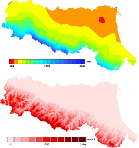
The south-eastern part of the region (named Romagna) is actually a different hydrographic region, since it is formed by rivers flowing directly in the Adriatic Sea, while the remain-ing catchments are all headwater tributaries to the Po River (the most important Italian river), belonging to the western part of the region (Emilia). Also the climate varies between the two areas from mountainous to maritime, going from the higher crests of the western side to the eastern coastal and hilly area. The western side of the region experiences more rain, with annual rainfall depths that exceed 2000 mm in the mountains, whereas the climate in the Romagna area changes due to the wind exposition, to the influence of the sea, to the lower orography and also to the lower latitude. Figure 1 shows mean annual precipitation depths and elevation of the Emilia-Romagna Region.

For each of the study catchments, time series data of hourly streamflow were collected for a total number of obser-vations ranging, for the different river sections, from 31 519 to 85 469 (that would correspond respectively to more than 3.5 and almost 10 yr of continuous monitoring but, as a mat-ter of fact, embrace periods of missing data). Hourly stream-flow data are expressed as spatial averaged runoff depths (mm h−1). Areal precipitation estimates, again at hourly step (mm h−1), were interpolated with Thiessen-polygon weight-ing from nearby rain-gauges.

2.2 Streamflow signatures

The first step of the proposed approach is to cluster the catch-ments on the basis of the hydrologic response, as defined by key signatures of the streamflow time series. The cho-sen signatures are (i) average runoff,µQ, (ii) the standard

deviation,σQ, and (iii–iv) the 5th and 95th percentiles,PQ,5

andPQ,95 of hourly data. To describe the correlation

struc-ture of the series, representing the dynamic component of the process, two metrics were computed: (v) the lag-1 autocor-relation coefficient,ρQ(1), and (vi) the correlation scaling

600 1400 2200

mm

0 1050 2150

[image:3.595.311.546.66.315.2]

m a.s.l.

Fig. 1. Mean annual precipitation (“Precipitazioni annue – Periodo 1991–2008”, ARPA Regione Emilia Romagna) and digital elevation model of the Emilia-Romagna region.

exponent (see for example Menabde et al., 1997, and Molnar and Burlando, 2008, for precipitation data, and the recent ap-plication by Ozger et al., 2012, to streamflow time series), that is the exponent that characterises the correlation func-tion with a power law:

ρQ(τ )∝τ−αQ, (1)

whereρQ is the autocorrelation function,τ is the time lag,

and αQ is the correlation scaling exponent. Values of αQ

tending to 0 indicate strongly correlated data, values close or higher than 1 show absence of correlation. Actually, the analysis of the correlation structures would require stationary time series, whereas streamflow observations (as well as rain-fall ones) exhibit a strong dependency on the season (see also the recent analysis by Patil and Stieglitz, 2011); to solve this problem, the above cited papers assume stationarity on a sea-sonal basis, estimating separate coefficients for the different seasons or months. In addition, if trends were present, Eq. (1) may not be capable of characterizing the structure of data in terms of multifractality and correlation dimension (see, e.g. Ozger et al., 2012). Nonetheless, due to the limited number of catchments in the data set, it was deemed appropriate, in this first study, to retain the smallest possible number of stream-flow signatures, in order to avoid over-parameterisation ef-fects in the classification technique; for this reason, even if acknowledging the strong limitations of this approximation, stationarity was hypothesised and only one value forαQwas

(4)

2.3 Catchment descriptors

In order to extend the analysis of the hydrological similar-ity also to catchments devoid of flow measurements, indexes describing the basins from the geo-morphological and clima-tological point of view are identified. The main geographical and morphometric attributes are derived from digital catch-ment boundaries coupled with the digital elevation model: (i)–(ii) the geographical coordinates UTM X andY of the stream gauges; (iii) drainage area,A, (iv)–(v) minimum and average catchment elevation,HminandHmed, and (vi) main

stream length,L. In addition, to better describe the catch-ments as far as the rainfall–runoff transformation is con-cerned, indexes obtained from the high-resolution areal rain-fall time series are estimated, thus attempting to characterise the fine time-scale variability and correlation structure of the precipitation process. The chosen pluviometric attributes are (i)–(ii) the mean and the standard deviation of the hourly data,µP andσP; (iii) the average proportion of wet hours

(hours with more than 0.2 mm of rain),PWet; finally, in

anal-ogy with the streamflow signatures, (iv) the lag-1 autocorre-lation coefficient,ρP(1), and (v) the correlation scaling

ex-ponent,αP, of the precipitation time series are computed.

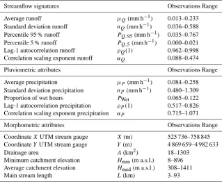
The chosen streamflow signatures and catchment at-tributes (pluviometric and morphometric) are listed in Ta-ble 1, along with the corresponding observation ranges over the data-set.

3 Classification of streamflow signatures with SOM neural networks

In the past three decades a number of applications of cluster analysis techniques have been presented in the hydrologic literature for the objective identification of catchments hav-ing similar attributes (either geographic, morphometric, cli-matic and/or based on streamflow observations). In the recent years, also non-supervised neural networks, and in particular of the SOM (self-organising mapping) type, were success-fully applied (and sometimes compared with other methods such as K-means or Fuzzy C-means) for catchments classi-fication purposes (Hall and Minns, 1999; Hall et al., 2002; Jingyi and Hall, 2004; Chang et al., 2008; Srinivas et al., 2008; Di Prinzio et al., 2011; Ley et al., 2011). SOM-type neural networks learn to cluster the input data by recogniz-ing different patterns organisrecogniz-ing the data on the basis of their similarity, quantified by means of a distance measure (in the present case, like in the majority of applications, the Eu-clidean distance). More details on the SOMs and in partic-ular on their use as classification techniques may be found for example in Herbst and Casper (2008) or in Toth (2009). The networks are formed by two layers of interconnected nodes (or neurons): each attribute of the entity to be clas-sified (i.e. a catchment) is fed to one of the input nodes, while the output nodes correspond to the classes to which the

entities are assigned. An input vectorx=(x1, x2, . . . , xn)

ac-tivates in fact only one output node, representing its class, us-ing the Kohonen competitive learnus-ing rule (Kohonen, 1997). Each output node is characterised by the weights connect-ing it to the input nodes. Initially the weights between the ninput nodes and each output node are randomly assigned. When, in the training phase, an input is sent through the net-work, each output neuron computes the distance between its weightsW =(w1, w2, . . . , wn)and the input vector:

kx−Wk = v u u t

n

X

i=1

(xi−wi)2. (2)

The output node responding maximally to the given input vector – specifically, the weights vector having the minimum distance from the input vector – is the winning neuron. At each training iterationt, the weights of the winning node and of its neighbouring nodes change, so to further reduce the distance between the weights and the input vector:

W(t+1)=W(t )+µ(t )hlm(x−W(t )), (3)

whereµis the learning rate,∈[0 1],landmare the positions of the winning and its neighbouring output nodes and hlm

is the neighbourhood shape, that reduces the adjustment for increasing distance, namely,

hlm=exp −

kl−mk2 2θ (t )2

!

, (4)

wherekl−mkis the lateral distance betweenlandmon the output grid andθis the width of the topological neighbour-hood.

Lateral interaction between neighbouring output nodes en-sures that learning is a topology-preserving process in which the network adapts to respond in different locations of the output layer for inputs that differ, while similar input patterns activate adjacent output units, corresponding to akin classes, as will be shown in the next subsections.

The values of the streamflow signatures (i.e. the input vec-tors) are standardized to zero mean and unit variance, so to give them equal importance in the evaluation of the distance measure.

The number of input variables (six in the present case) cor-responds to the dimension of the input layer, whereas the di-mension of the output layer is equal to the number of classes to be determined.

3.1 SOM classification in 6 clusters

(5)

[image:5.595.136.456.82.344.2]

Table 1. Streamflow signatures, pluviometric and morphometric attributes.

Streamflow signatures Observations Range

Average runoff µQ(mm h−1) 0.013–0.233

Standard deviation runoff σQ(mm h−1) 0.036–0.588

Percentile 95 % runoff PQ,95(mm h−1) 0.035–0.767

Percentile 5 % runoff PQ,5(mm h−1) 0.000–0.021

Lag-1 autocorrelation runoff ρQ(1) 0.962–0.998

Correlation scaling exponent runoff αQ 0.088–0.474

Pluviometric attributes Observations Range

Average precipitation µP (mm h−1) 0.084–0.258

Standard deviation precipitation σP (mm h−1) 0.480–1.309

Proportion of wet hours PWet 0.065–0.122

Lag-1 autocorrelation precipitation ρP(1) 0.517–0.826

Correlation scaling exponent precipitation α_P 0.715–1.071

Morphometric attributes Observations Range

CoordinateXUTM stream gauge X(m) 525 736–758 845 CoordinateYUTM stream gauge Y (m) 4 869 659–4 982 633

Drainage area A(km2) 18–1303

Minimum catchment elevation Hmin(m a.s.l.) 8–896

Average catchment elevation H_med(m a.s.l.) 308–1411

Main stream length L(km) 3–93

In the present work, a first SOM application partitions the streamflow attributes vectors into six classes, i.e. in a rela-tively large (in reference to the number of entities to be clas-sified) number of groups, aiming at a sufficiently detailed discrimination between the classes, so to highlight the most important features of the data drawn from the input space. The SOM may in fact be seen also as an information content extractor, projecting the analysed entities (streamflow signa-tures vectors) on the output layer, which has a lower dimen-sion (2-dim) than that of the inputs (6-dim). The SOM output layer is set equal to 3×2 nodes, corresponding to 6 clusters of similar catchments organised on a hexagonal lattice, so that diagonal neighbours have the same distance as horizontal and vertical ones.

When the training is complete, each vector of streamflow signatures is assigned to its winning node, that corresponds to the class. Figure 2 shows the closure sections of the catch-ments associated to the six obtained clusters, along with a representation of the hexagonal output layer.

Following the presentation methodology proposed in Chang et al. (2010), a topology map is presented in Fig. 3. Such a map shows the mean value of each streamflow at-tribute (standardised to zero mean and unit variance) for the catchments of each cluster.

The topology, that is the relative location of the nodes, allows to visualise the variation of the streamflow features along the different classes, characterising the behaviour of the input variables and their interrelations. Class A (top-left hand corner) corresponds to the catchments with the maxi-mum runoff, having the highest values ofµQ,σQ,PQ,5and

PQ,95. The adjacent cluster B retains values of PQ,5 and

PQ,95 higher than the regional average (even if to a lesser

extent than Class A), whereasµQandσQare very close to

the mean (zero) value. In Class C, which is adjacent to both A and B, but also to the remaining three classes, all the stream-flow signatures are squeezed close to the mean values. On the other hand (and on the opposite part of the lattice), groups D, E and especially F (the furthest from the most humid cluster A) correspond to the catchments with the lowest runoff, with negative standardised values ofµQ,σQ,PQ,5andPQ,95.

When considering the indexes devised for representing the dynamic component of the process, we can identify the most highly correlated streamflows (largeρQ(1)and small αQ),

on the top-right hand side (Classes B and D), whereas the less temporally correlated ones (very low values of ρQ(1)

and high αQ) characterise Class E, on the opposite corner.

Classes A and C (top-left corner) haveρQ(1)andαQclose to

the regional mean and the bottom right-hand corner (F) lies in between its neighbours E and D, with positive (standardised) values for bothαQandρQ(1).

The topology map evidences the core morphological and climatological features of the different groups of catchments, as may be inferred from their geographical location, compar-ing Fig. 2 with Fig. 1: the top-left hand class A (black dia-monds) is formed by very rainy but small (due to the reduced size, the streamflow is not strongly correlated) catchments: they are located in the mountainous (southern) part of the western area.

(6)

E C A

D

[image:6.595.311.544.60.281.2]

F B

Fig. 2. Catchments of the 6-cluster classification identified by SOM based on streamflow signatures.

show a significant temporal correlation: they are located in the western (more rainy) region too, but more downstream, and have larger areas, so that both the humid climate and the size induce a significant correlation.

Classes F and D (bottom right-hand side) correspond to the less humid catchments: to the first class belong those – from east to west – at lower altitudes (see the position of the red di-amonds, in the piedmont or flat part of the region), where the impact of orographic precipitation is limited; the elements of D (yellow) are instead almost all located in the eastern, cli-matologically less rainy, part of the region (Romagna).

Cluster E (orange) is formed by small basins (the size is consistent on the lattice topology, since the nodes on the left side, A and E, correspond to the smallest catchments) with modest runoff, characterised by the lowest temporal correla-tion.

Lastly, class C is the less markedly characterised, with all streamflow indexes close to the regional averages, as topo-logically consistent with its position on the lattice, being the neuron that is at equal distance from all the other five. Such more “amorphous” catchments are a minority, four in total, whereas the other groups are formed by 7 to 9 elements, high-lighting a good balance in the numerousness of the classes.

3.2 SOM classification in 3 clusters

A second SOM application was set up for partitioning the watersheds in three, instead of six, classes. In fact the dis-criminant analysis to be performed in the second part of the study – aimed at assigning ungauged catchments to the classes identified as a function of the streamflow signatures – needs a less detailed clustering resolution, in order to avoid the effects of overparameterisation. In detail, the number of discriminant variables multiplied by the number of classes should be not greater than one fourth of the total number of records (Hand, 1997; Sanborn and Bledsoe, 2006).

It was hence decided, in this second classification ex-periment, to limit to three the number of hydrologically

-2.0 -1.0 0.0 1.0 2.0

µQ σQPQ,95PQ,5ρQ αQ -2.0 -1.0 0.0 1.0 2.0

µQ σQPQ,95PQ,5ρQ αQ

-2.0 -1.0 0.0 1.0 2.0

µQ σQPQ,95PQ,5ρQ αQ -2.0 -1.0 0.0 1.0 2.0

-2.0 -1.0 0.0 1.0 2.0

µQ σQPQ,95PQ,5ρQ αQ -2.0 -1.0 0.0 1.0 2.0

-2.0 -1.0 0.0 1.0 2.0

A B

C D

E F

Fig. 3. Topology map of 6-cluster (3×2) SOM classification of streamflow signature vectors.

homogeneous clusters, with an output layer consisting of only 3 nodes.

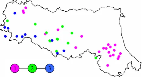
Figure 4 indicates the closure sections of the catchments associated to each of the three classes, whereas the topology map (Fig. 5) shows the mean value – for each cluster – of the standardised streamflow attributes.

The trained network associates to Class 1 (magenta) al-most half of the study catchments (21 over 44) formed by the previous (6-cluster) adjacent classes F and D, plus the major-ity of class E (contiguous to F). Consistently with the more refined partitioning, such catchments are those that generate the lowest runoff (small values ofµQ,PQ,5,PQ,95andσQ,

as illustrated in the topology map).

It may be observed in Fig. 4 that Class 1 includes almost all the basins of the south-eastern part of the study area (Ro-magna) and other lower-altitude and drier catchments located in the downstream (northern) part of the western valleys. It is realistic that the Romagna catchments – that are close to each other and belong, as said in Sect. 2.1, to a distinct hydro-graphic region – seem to behave in a hydrologically similar way according to this second, coarser classification. In fact such a contiguous area is certainly characterised by similar climate, topography and geology, and all other characteris-tics deriving from them, such as soil type, vegetation, etc. (Merz and Bloeschl, 2005; Patil et al., 2012).

On the other hand it is evident, as expectable, that the coarser clustering is not able to fully capture the differences among the hydrometric signatures, and in particular among the dynamic components of the streamflow process. Class 1 in fact is characterised, on average, by series that are slightly less autocorrelated than the regional averages (smallerρQ(1)

[image:6.595.51.286.60.198.2]

(7)

2 3 1 1

2 3

[image:7.595.309.545.63.139.2]

1

Fig. 4. Catchments of the 3-cluster classification identified by SOM based on streamflow signatures.

different temporal correlation indexes: the less correlated ones (belonging to Class E of the 6-cluster grouping) along with time series that are instead more correlated (Class D) or characterised by a mixed condition (Class F, having both ρQ(1)andαQvalues above the regional averages). As a

con-sequence, the autocorrelation coefficient and the correlation scaling exponent have limited discriminant power in the 3-cluster analysis.

Class 3 (11 elements) incorporates the 6-cluster Class A and a part of Class B, corresponding to the highest runoff (as evidenced by the topology maps) and to a temporal correla-tion which is, on average, slightly higher than the regional means. Consistently with the geographical location of the el-ements of Class A (and Class B), Class 3 mainly includes the mountainous catchments of the western area, characterised by higher altitude and precipitation.

Finally, Class 2 (12 catchments) stands in between the other two clusters, adding to the “amorphous” Class C the catchments of Class E that fit less in the new 3-cluster Class 1 and a few from Classes B and D that do not fit in Class 3.

Comparing the results of the two classifications (6-cluster and 3-cluster), it is demonstrated that the topological order of the SOM structure guarantees that solutions with more clusters are correctly nested within the solutions that have fewer clusters. On the other hand, the coarser classification is mainly led by the signatures representing runoff magni-tude and, while it clearly separates the higher and lower val-ues ofµQ,PQ,5,PQ,95andσQ, those ofρQ(1)andαQare,

instead, extremely variable inside each class, indicating that the dynamic component of the process is not given sufficient consideration.

Despite the above mentioned limitation, the SOM classifi-cations (both 3-cluster and 6-cluster) based on streamflow signatures seem overall to indicate a good grouping abil-ity, as highlighted by the consistent interpretation of how the main features of the input variables vary in the differ-ent classes and of their interrelations, as illustrated through the analysis of their topology maps. In addition, even if no geographical, morphological nor climatological information

-1.5 -1.0 -0.5 0.0 0.5 1.0 1.5

µQσQPQ,95PQ,5ρQαQ -1.5 -1.0 -0.5 0.0 0.5 1.0 1.5

µQσQPQ,95PQ,5ρQαQ

[image:7.595.51.286.65.191.2]

1 2 3

Fig. 5. Topology map of 3-cluster SOM classification of streamflow signatures vectors.

is provided in input to the SOM network, the clusters exhibit an overall consistency as far as location, altitude and precip-itation regime are concerned.

4 Application to ungauged catchments

One of the primary practical objectives for delineating hy-drological homogeneous regions is to assess the member-ship of ungauged sites, thus inferring indications on the re-sponse behaviour of such catchments. An important feature of a cluster analysis aimed at identifying homogeneous clus-ters is therefore the ability to discriminate between them on the basis of variables that are different from the streamflow signatures, namely, a set of physical and climatic character-istics of the watersheds. In Sect. 3, the SOM was applied as an unsupervised methodology for grouping together catch-ments that are similar from the hydrometric point of view. The objective of the methodology presented in this section is to assign to such classes any new watershed where the streamflow attributes are not available. A discriminant analy-sis is applied as a supervised learning technique, that assigns each record to predefined groups. To this end, it constructs a classification rule based on the knowledge, for the same catchments, of (i) the morphologic and pluviometric proper-ties presented in Sect. 2.3 (chosen as discriminant) and (ii) the hydrometric class: the clusters obtained by the unsuper-vised 3-cluster SOM based on streamflow indexes become, in this second analysis, the predefined reference classifica-tion. The goodness of the discriminant analysis is then as-sessed through the capability of assigning a catchment, on the basis of its morpho-pluviometric attributes only, to the same class to which it would be assigned if its streamflow at-tributes were known. This approach is similar to that applied by Bhaskar and O’Connor (1989), Chiang et al. (2002) and Sanborn and Bledsoe (2006), albeit with different hydromet-ric and morpho-climatic sets of indices and different cluster analysis techniques.

4.1 Principal component analysis of catchment descriptors

(8)

[image:8.595.318.537.62.181.2]

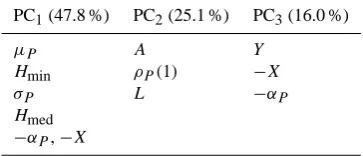
Table 2. Morpho-pluviometric variables with the highest loadings on the first three PCs and total explained variance (in parentheses).

PC₁(47.8 %) PC₂(25.1 %) PC₃(16.0 %)

µP A Y

Hmin ρP(1) −X

σP L −αP

Hmed

−αP,−X

σP, PWet, ρP(1), αP). Also due to the above cited

over-parameterisation constraints, the catchment descriptor vec-tors are subjected to a principal component analysis to iden-tify a smaller number of uncorrelated variables that describe the dominant patterns of variance in the data.

The principal component analysis shows how the first three principal components (PCs) explain, together, 89 % of the total variance (and the fourth one adds only another 4.6 % of explanation). Table 2 presents the original variables that mostly affect the first three PCs (i.e. those with the highest loadings) and the percentage of total variance explained by each PC.

The principal component analysis helps to interpret the differences and similarities of the data; in fact each PC de-scribes a specific aspect of the variability of the catchment attributes and the variables with the highest loadings on a PC best explain that “dimension” of the data (Chiang et al., 2002; Sanborn and Bledsoe, 2006). The first PC is positively asso-ciated withHmin, Hmed,µP,σP, thus representing the

in-fluence of elevation, corresponding to higher rainfall values (due to orographic effect), whereas the correlation scaling exponent,αP (and also the X coordinate, since the eastern

part of the study region is less markedly rugged and receives less rainfall) contributes with the opposite sign, and there-fore with lower values (associated to higher correlation) for increasing altitude. This result is consistent with the findings of Molnar and Burlando (2008), where the most elevated ar-eas exhibit lowerαP-values (and therefore a stronger

corre-lation, indicating that the orographic forcing leads to better organised and long-lasting precipitation fields). The second PC, associated toA,L andρP(1), substantially represents

the catchment dimension, increasing along with the lag-1 autocorrelation of the spatially averaged rainfall. The third component, associated with negativeX and positiveY val-ues, represents the geographical location; moving along the Apennine ridge from SE to NW,αP decreases. This shows

that the precipitation on the Emilia area tends to be more tem-porally correlated than that on the Romagna area, the latter being less mountainous and less rainy, due also to the influ-ence of the sea and of the southern currents.

2 3 1 1

[image:8.595.75.257.94.172.2]

2 3 1

Fig. 6. Classification identified by discriminant analysis based on the first three PCs of the catchment descriptors.

4.2 Discriminant analysis for classification of ungauged catchments

Discriminant analysis is a supervised learning technique that treats a set of observations with one classification variable and one or more quantitative variables (or discriminants) to describe each classified entity. On the basis of such informa-tion, the algorithm constructs a classification rule as a func-tion of the quantitative variables that allows to assign any new record to one of the predefined groups. The analysis identifies the combination of the quantitative variables that maximises the ratio between the inter-classes variance and the intra-classes variance (thus maximising the inter-class separability and the intra-class compactness of the data sam-ples in a low-dimensional vector space), finding the one that can most effectively partition the predefined groups (Hand, 1981; Krzanowski, 1988).

In the present application, the quantitative variables de-scribing each entity are the first three principal compo-nents of the catchment descriptors (presented above) and the classes are the three clusters identified by the SOM network based on the streamflow signatures (see Sect. 3.2). This is consistent with the indications (cited in the same section) that, for an optimal discriminant analysis, it is preferable that the number of discriminant variables multiplied by the num-ber of classes is less than one fourth of the total numnum-ber of records to be classified (44 in the present case).

The discriminant capacity is assessed through the com-parison between the streamflow signatures classification and the one derived by the catchment attributes. It was here per-formed a leave-one-out cross validation, considering, in turn, each basin as ungauged and therefore excluding it from the data used to construct the discriminant criterion. It is finally possible to determine the percentage of gauged sites correctly classified in the discriminant-based approach. The classifica-tion obtained with the discriminant analysis is represented in Fig. 6.

(9)

between Class 1 and Class 2. It is worthy observing that there are no instances in which catchments belonging to Class 1 are assigned to Class 3 or the other way round. This is a merit of the topological properties of the SOM network, unique among the other clustering techniques: the relative position of the nodes on the output layer allows, indeed, to take into consideration the affinity among the classes, since nodes that are nearby may be considered representative of akin classes. Classes 1 and 3 correspond, in fact, to the less similar groups, while Class 2 is intermediate between the two. It is hence comforting to observe that the two most different clusters re-sult separately in both classifications and that the only errors are exchanges with the intermediate cluster.

5 Conclusions

The methodology developed in this study first provides a means for identifying groups of similar catchments on the basis of streamflow indexes (signatures) and successively classifies, in the same clusters, ungauged basins on the basis of climate and landscape characteristics. The main novelty of the approach lies in the inclusion, both in the streamflow and in the rainfall characterisation, of information derived by the fine-scale continuous time series, through indexes attempt-ing to synthesise, in a parsimonious way, the variability and correlation structure of the respective processes.

The streamflow signatures are fed to two unsupervised self-organising mapping networks, forming respectively 3 and 6 groups of similar catchments, and obtaining – espe-cially for the more refined 6-cluster partition – classes with a clear hydrological distinctiveness. This is highlighted not only by the consistent interpretation of how the main features of the input variables vary in the different classes and of their multi-relations (shown by the topology maps), but also by the spatial distribution of the groups of homogeneous catch-ments. In fact, even if no geographical, morphological nor climatological information is provided in input to the SOM network, the clusters exhibit an overall consistency as far as location, altitude and precipitation regime are concerned.

On the other hand, as expected, the coarser clustering is not able to fully capture the differences among the hydromet-ric signatures, and in particular among the dynamic compo-nents of the streamflow process: the 3-cluster classification is in fact mainly led by the signatures representing runoff magnitude but it merges basins characterised by very differ-ent temporal correlation indexes, indicating that the dynamic component of the process is not given sufficient considera-tion.

In order to classify new observations (ungauged sites) to an appropriate streamflow response group, a set of morpho-logic and pluviometric attributes are identified for describ-ing each catchment. The analysis of the principal compo-nents (PCs) of the morpho-pluviometric attributes shows that each of the first three PCs seems able to represent a specific

aspect of the differences among the catchments, highlighting, in particular, the role and the dependence among the vari-ables characterising the precipitation regime and its correla-tion structure.

The limited data set prevented the use of the more de-tailed (6-cluster) classification in the discriminant analysis (applied for assigning ungauged catchments to the predeter-mined SOM classes based on streamflow signatures), due to over-parameterisation constraints, but it is intended, in future work, to try to enlarge the number of study catchments for al-lowing also such investigation.

The results of the discriminant analysis, that identifies the membership of ungauged catchments (described by the corresponding three first PCs) in a leave-one-out cross-validation scheme, evidence a quite satisfactory agreement with the 3-cluster SOM classification that is assumed as a reference partition. Moreover, the discriminant analysis clus-tering is able to clearly distinguish the two less similar groups (Class 1 and Class 3) identified in the streamflow-based SOM classification: in fact all the misclassification errors are ex-changes with the intermediate Class 2.

Of course it is arduous aspiring at a fully appropriate hy-drological classification with the set of catchment attributes that are available for this study. For a better characterisation of the phenomena governing the streamflow process, a more comprehensive data set would be needed, including informa-tion on the geo-pedological, vegetainforma-tion and land-use proper-ties of the drainage areas, as well as additional climatic in-dexes.

In addition, the chosen signatures represent a very simpli-fied description of the autocorrelation function and in partic-ular the assumption of stationarity is indeed a relevant ap-proximation, given the strong seasonality of the streamflow process. It would be worthy, provided that a larger sample of streamflow time series is available, to provide a more refined representation of the correlation structure, in particular for testing the potential advantages of a seasonal interpretation of the data.

Notwithstanding all the above cited limitations, the results confirm the potential of the proposed approach for charac-terising the catchments. The inclusion of information on the properties of the fine time-scale streamflow and rainfall time series appears a promising way for better delineating the hy-drologic and climatic character of the catchments, at least as far as the present study area is concerned.

Acknowledgements. Analyses are based on measurements

pro-vided by the Regional Civil Protection Agency and by the Hydro-Meteorological Service of the Environmental Agency of Emilia-Romagna Region. The author also thanks Alberto Viglione and two anonymous reviewers for their constructive comments and helpful suggestions.

(10)

References

Atkinson, S. E., Woods, R. A., and Sivapalan, M.: Climate, soil, vegetation controls on water balance model complex-ity over changing timescales, Water Resour. Res., 38, 1314, doi:10.1029/2002WR001487, 2002.

Bhaskar, N. R. and O’Connor, C. A. : Comparison of method of residuals and cluster analysis for flood regionalization, J. Water Resour. Pl.-ASCE, 115, 793–808, 1989.

Burn, D. H.: Cluster analysis as applied to regional floood fre-quency, J. Water Resour. Pl.-ASCE, 115, 567–582, 1989. Burn, D. H. and Goel, N. K.: The formation of groups for regional

flood frequency analysis, J. Hydrol. Sci., 45, 97–112, 2000. Burn, D. H., Zrinji, Z., and Kowalchuk, M.: Regionalization of

catchments for regional flood frequency analysis, J. Hydrol. Eng., 2, 76–82, 1997.

Castellarin, A., Brath, A., and Burn, D.: Assessing the effectiveness of hydrological similarity measures for flood frequency analysis, J. Hydrol., 241, 270–285, 2001.

Castiglioni, S. Lombardi, L., Toth, E., Castellarin, A. and Mon-tanari, A.: Calibration of rainfall-runoff models in ungauged basins: A regional maximum likelihood approach, Adv. Water Resour., 2010, 33, 1235–1242, 2010.

Chang, F. J., Tsai, M. J., Tsai, W. P., and Herricks, E. E.: Assessing the Ecological Hydrology of Natural Flow Conditions in Taiwan, J. Hydrol., 354, 75–89, 2008.

Chang, F. J., Chang, L. C., Kao, H. S., and Wua, G. R.: Assess-ing the effort of meteorological variables for evaporation esti-mation by self-organizing map neural network, J. Hydrol., 384, 118–129, 2010.

Chiang, S. M., Tsay, T. K., and Nix, S. J.: Hydrologic regionaliza-tion of watershed. Part I. Methodology development, J. Water Resour. Pl.-ASCE, 128, 1–11, 2002.

Corduas, M.: Clustering streamflow time series for regional classi-fication, J. Hydrol, 407, 73–80, 2011.

De Thomasis, E. and Grimaldi, S.: Introduzione di una metrica tra modelli parametrici lineari nelle applicazioni di tipo idro-logico, Giornata di Studio: Metodi Statistici and Matematici per l’Analisi delle Serie Idrologiche, Roma, 2001 (in Italian). Di Prinzio, M., Castellarin, A., and Toth, E.: Data-driven

catch-ment classification: application to the pub problem, Hydrol. Earth Syst. Sci., 15, 1921–1935, doi:10.5194/hess-15-1921-2011, 2011.

Grimaldi, S.: Linear parametric models applied to daily hydrologi-cal series, J. Hydrol. Eng., 9, 383–391, 2004.

Haines, A. T., Finlayson, B. L., and McMahon, T. A.: A global clas-sification of river regimes, Appl. Geogr., 8, 255–272, 1988. Hall, M. J. and Minns, A. W.: The classification of hydrological

homogeneous regions, J. Hydrol. Sci., 44, 693–704, 1999. Hall, M. J., Minns, A. W., and Ashrafuzzaman, A. K. M.: The

ap-plication of data mining techniques for the regionalisation of hydrological variables, Hydrol. Earth Syst. Sci., 6, 685–694, doi:10.5194/hess-6-685-2002, 2002.

Hand, D. J.: Discrimination and Classification, John Wiley and Sons, Inc., New York, 218 pp., 1981.

Hand, D. J.: Construction and Assessment of Classification Rules, Wiley, Chichester, England, 214 pp., 1997.

Herbst, M. and Casper, M. C.: Towards model evaluation and iden-tification using Self-Organizing Maps, Hydrol. Earth Syst. Sci., 12, 657–667, doi:10.5194/hess-12-657-2008, 2008.

Holmes, M. G. R., Young, A. R., Gustard, A., and Grew, R.: A new approach to estimating Mean Flow in the UK, Hydrol. Earth Syst. Sci., 6, 709–720, doi:10.5194/hess-6-709-2002, 2002.

Hosking, J. R. M., Wallis, J. R., and Wood, E. F.: An appraisal of the regional flood frequency procedure in the UK “Flood Studies Report”, Hydrolog. Sci. J., 30, 85–109, 1985.

Jingyi, Z. and Hall, M. J.: Regional flood frequency analysis for the Gan-Ming River basin in China, J. Hydrol., 296, 98–117, 2004. Kohonen, T.: Self-Organizing Maps, 2nd Edn., Springer, 1997. Krzanowski, W. J.: Principles of Multivariate Analysis, A User’s

perspective, Oxford Univ. Press, New York, 612 pp., 1988. Laaha, G. and Bloeschl, G.: A comparison of low flow

regionaliza-tion methods – catchment grouping, J. Hydrol., 323, 193–214, 2006.

Lettenmeier, D. P., Wallis, J. R., and Wood, E. F.: Effect of regional heterogeneity on flood frequency estimation, Water Resour. Res., 23, 313–323, 1987.

Ley, R., Casper, M. C., Hellebrand, H., and Merz, R.: Catch-ment classification by runoff behaviour with self-organizing maps (SOM), Hydrol. Earth Syst. Sci., 15, 2947–2962, doi:10.5194/hess-15-2947-2011, 2011.

Lombardi, L., Toth, E., Castellarin, A., Montanari, A., and Brath, A.: Calibration of a rainfall-runoff model at regional scale by optimising river discharge statistics: performance analysis for the average/low flow regime, Phys. Chem. Earth, 42–44, 77–84, 2012.

Marani, M.: On the correlation structure of continuous and discrete point rainfall, Water Resour. Res., 39, 1128, doi:10.1029/2002WR001456, 2003.

McDonnell, J. J. and Woods, R. A.: On the need for catchment clas-sification, J. Hydrol., 299, 2–3, 2004.

Menabde, M., Harris, D., Seed, A., Austin, G., and Stow, D.: Multi-scaling properties of rainfall and bounded random cascades, Wa-ter Resour. Res., 33, 2823–2830, 1997.

Merz, R. and Bloeschl, G.: Flood frequency regionalization: spa-tial proximity vs. catchment attributes, J. Hydrol., 302, 283–306, 2005.

Molnar, P. and Burlando P.: Variability in the scale prop-erties of high-resolution precipitation data in the Alpine climate of Switzerland, Water Resour. Res., 44, W10404, doi:10.1029/2007WR006142, 2008.

Montanari, A. and Toth, E.: Calibration of hydrological models in the spectral domain: An opportunity for scarcely gauged basins?, Water Resour. Res., 43, W05434, doi:10.1029/2006WR005184, 2007.

Nathan, R. J. and McMahon, T. A.: Identification of homogeneous regions for the purpose of regionalization, J. Hydrol., 121, 217– 238, 1990.

Oudin, L., Kay, A., Andreassian, V., and Perrin, C.: Are seemingly physically similar catchments truly hydrologically similar?, Wa-ter Resour. Res., 46, W11558, doi:10.1029/2009WR008887, 2010.

(11)

Patil, S. and Stieglitz, M.: Controls on hydrologic similarity: role of nearby gauged catchments for prediction at an ungauged catch-ment, Hydrol. Earth Syst. Sci., 16, 551–562, doi:10.5194/hess-16-551-2012, 2012.

Piacentini, T., Castaldini, D., Coratza, P., Farabollini, P., and Mic-cadei, E.: Geotourism: Some examples in Northern-Central Italy, GeoJournal of Tourism and Geosites, Year IV no. 2, 8, 240–262, 2011.

Samaniego, L., Bardossy, A., and Kumar, R.: Streamflow prediction in ungauged catchments using copula-based dissimilarity measures, Water Resour. Res., 46, W02506, doi:10.1029/2008WR007695, 2010.

Sanborn, S. C. and Bledsoe, B. P.: Predicting streamflow regime metrics for ungauged streams in Colorado, Washington, Oregon, J. Hydrol., 325, 241–261, 2006.

Sauquet, E. and Catalogne, C.: Comparison of catchment group-ing methods for flow duration curve estimation at ungauged sites in France, Hydrol. Earth Syst. Sci., 15, 2421–2435, doi:10.5194/hess-15-2421-2011, 2011.

Sawicz, K., Wagener, T., Sivapalan, M., Troch, P. A., and Carrillo, G.: Catchment classification: empirical analysis of hydrologic similarity based on catchment function in the eastern USA, Hy-drol. Earth Syst. Sci., 15, 2895–2911, doi:10.5194/hess-15-2895-2011, 2011.

Singh, R. D., Mishra, S. K., and Chowdhary, H.: Regional flow-duration models for large number of ungauged Himalayan catch-ments for planning microhydro projects, J. Hydrol. Eng., 6, 310– 316, 2001.

Srinivas, V. V., Tripathi, S., Rao, A. R., and Govindaraju, R. S.: Regional flood frequency analysis by combining self-organizing feature map and fuzzy clustering, J. Hydrol., 348, 148–166, 2008.

Thomas, B., Lischeid, G., Steidl, J., and Dannowski, R.: Regional catchment classification with respect to low flow risk in a Pleis-tocene landscape, J. Hydrol., 475, 392–402, 2012.

Toth, E.: Classification of hydro-meteorological conditions and multiple artificial neural networks for streamflow forecasting, Hydrol. Earth Syst. Sci., 13, 1555–1566, doi:10.5194/hess-13-1555-2009, 2009.

Vezza, P., Comoglio, C., Rosso, M., and Viglione, A.: Low Flows Regionalization in North-Western Italy, Water Resour. Manage., 24, 4049–4074, 2010.

Viglione, A., Claps, P., and Laio, F.: Mean Annual Runoff Estima-tion in North-Western Italy, in: Water resources assessment and management under water scarcity scenarios, edited by: La Log-gia, G., CDSU Publ. Milano, Italy, 2006.

Wagener, T., Sivapalan, M., Troch, P., and Woods, R.: Catchment Classification and Hydrologic Similarity, Geogr. Compass, 1, 901–931, doi:10.1111/j.1749-8198.2007.00039.x, 2007. Yilmaz, K. K., Gupta, H. V., and Wagener, T.: A process based