Hydrol. Earth Syst. Sci., 17, 2809–2825, 2013 www.hydrol-earth-syst-sci.net/17/2809/2013/ doi:10.5194/hess-17-2809-2013
© Author(s) 2013. CC Attribution 3.0 License.
EGU Journal Logos (RGB)
Advances in
Geosciences
Open Access
Natural Hazards
and Earth System
Sciences
Open Access
Annales
Geophysicae
Open Access
Nonlinear Processes
in Geophysics
Open Access
Atmospheric
Chemistry
and Physics
Open Access
Atmospheric
Chemistry
and Physics
Open Access
Discussions
Atmospheric
Measurement
Techniques
Open Access
Atmospheric
Measurement
Techniques
Open Access
Discussions
Biogeosciences
Open Access Open Access
Biogeosciences
Discussions
Climate
of the Past
Open Access Open Access
Climate
of the Past
Discussions
Earth System
Dynamics
Open Access Open Access
Earth System
Dynamics
Discussions
Geoscientific
Instrumentation
Methods and
Data Systems
Open Access
Geoscientific
Instrumentation
Methods and
Data Systems
Open Access
Discussions
Geoscientific
Model Development
Open Access Open Access
Geoscientific
Model Development
Discussions
Hydrology and
Earth System
Sciences
Open Access
Hydrology and
Earth System
Sciences
Open Access
Discussions
Ocean Science
Open Access Open Access
Ocean Science
Discussions
Solid Earth
Open Access Open Access
Solid Earth
Discussions
The Cryosphere
Open Access Open Access
The Cryosphere
DiscussionsNatural Hazards
and Earth System
Sciences
Open Access
Discussions
Using a thermal-based two source energy balance model with
time-differencing to estimate surface energy fluxes with day–night
MODIS observations
R. Guzinski1, M. C. Anderson2, W. P. Kustas2, H. Nieto1, and I. Sandholt1
1Department of Geosciences and Natural Resource Management, University of Copenhagen, Øster Voldgade 10,
1350 Copenhagen, Denmark
2Hydrology Laboratory, Agriculture Research Service, US Department of Agriculture, Beltsville, Maryland, USA Correspondence to: R. Guzinski (rag@geo.ku.dk)
Received: 22 January 2013 – Published in Hydrol. Earth Syst. Sci. Discuss.: 11 February 2013 Revised: 24 May 2013 – Accepted: 16 June 2013 – Published: 16 July 2013
Abstract. The Dual Temperature Difference (DTD) model,
introduced by Norman et al. (2000), uses a two source en-ergy balance modelling scheme driven by remotely sensed observations of diurnal changes in land surface temperature (LST) to estimate surface energy fluxes. By using a time-differential temperature measurement as input, the approach reduces model sensitivity to errors in absolute temperature retrieval. The original formulation of the DTD required an early morning LST observation (approximately 1 h after sun-rise) when surface fluxes are minimal, limiting application to data provided by geostationary satellites at sub-hourly tem-poral resolution. The DTD model has been applied primar-ily during the active growth phase of agricultural crops and rangeland vegetation grasses, and has not been rigorously evaluated during senescence or in forested ecosystems. In this paper we present modifications to the DTD model that enable applications using thermal observations from polar or-biting satellites, such as Terra and Aqua, with day and night overpass times over the area of interest. This allows the ap-plication of the DTD model in high latitude regions where large viewing angles preclude the use of geostationary satel-lites, and also exploits the higher spatial resolution provided by polar orbiting satellites. A method for estimating noc-turnal surface fluxes and a scheme for estimating the frac-tion of green vegetafrac-tion are developed and evaluated. Mod-ification for green vegetation fraction leads to significantly improved estimation of the heat fluxes from the vegetation canopy during senescence and in forests. When the modified DTD model is run with LST measurements acquired with the
Moderate Resolution Imaging Spectroradiometer (MODIS) on board the Terra and Aqua satellites, generally satisfactory agreement with field measurements is obtained for a number of ecosystems in Denmark and the United States. Finally, re-gional maps of energy fluxes are produced for the Danish Hydrological ObsErvatory (HOBE) in western Denmark, in-dicating realistic patterns based on land use.
1 Introduction
Over the past 35 yr, a wide variety of approaches have been developed to model the surface energy balance us-ing satellite-derived observations of land surface temperature (LST) (Kalma et al., 2008), with ongoing work in a number of techniques such as the triangle method (de Tom´as et al., 2012) or one source energy balance models (Boulet et al., 2012). One of the more robust modelling approaches is the two source energy balance (TSEB) thermal-based modelling scheme, which explicitly treats the energy fluxes emanating from the soil and canopy and partitions the observed LST between the two components based on the fractional area they each occupy in the LST pixel (Norman et al., 1995). The TSEB scheme has been successfully applied for esti-mating surface latent and sensible heat fluxes at regional to continental scales using geostationary satellite surface ra-diometric temperature observations within a regional mod-elling system called the Atmospheric Land-EXchange In-verse (ALEXI) model (Anderson et al., 2007). The ALEXI
modelling system addresses a critical limitation of thermal-based energy balance models regarding sensitivity to errors in absolute measurements of LST, which can be on the order of several degrees when derived from satellites due to atmo-spheric and surface emissivity effects. ALEXI reduces this sensitivity by using a time-differential measurement – the change of LST between two observations during the morn-ing growth phase of the atmospheric boundary layer – which can be retrieved with better accuracy. An associated spatial disaggregation technique, DisALEXI (Norman et al., 2003), uses LST data from polar orbiting satellites to improve the spatial resolution of the modelled flux images for use in a va-riety of operational applications (Anderson et al., 2012a).
The Dual-Temperature Difference (DTD) model, intro-duced by Norman et al. (2000), also addresses the issue of sensitivity of thermal-based models to errors in absolute measurements of LST. Like ALEXI, the DTD also requires two LST observations – one early in the morning and one later in the morning or in the afternoon. However, a simpler solution scheme is employed, thereby reducing the number of required inputs and model complexity in comparison with ALEXI. The original model formulation requires an early morning LST observation (approximately 1 h after local sun-rise) when fluxes are usually minimal. This means that, like ALEXI, it is dependent on the high temporal resolution of geostationary satellite measurements, which is unsuitable for applications at higher latitudes, such as in northern Eurasia and northern North America, where the view zenith angle (VZA) from geostationary satellites is large, causing loss of spatial resolution and accuracy due to longer atmospheric path lengths. These same issues also affect DisALEXI, which relies on the availability of ALEXI-derived fluxes as the nor-malization basis for disaggregation. The DTD has been eval-uated primarily in rangelands and croplands during the grow-ing season but before the onset of senescence. Therefore, its accuracy in forested ecosystems or other phenological stages is unknown.
In this paper, modifications to the DTD model are pre-sented that enable it to be used with LST observations from the Moderate Resolution Imaging Spectroradiometer (MODIS) sensor aboard the Terra and Aqua polar orbiting satellites, facilitating regional surface energy flux modelling over boreal regions. First, a scheme for estimating the frac-tion of vegetafrac-tion that is green,fg, using MODIS vegeta-tion indices is evaluated. The green fracvegeta-tion is an impor-tant parameter within the model, and is used to adjust esti-mates of canopy transpiration based on a modified Priestley– Taylor approach (Norman et al., 2000). Incorporating the green fraction parameterization improves DTD model accu-racy in forested ecosystems and during senescence by tak-ing into account the phenological development of the veg-etation. Next, a method for modelling the nocturnal energy fluxes is developed, taking advantage of the fact that the Terra and Aqua satellites combined provide at least two nightly and two daily acquisitions every 24 h. Finally, we consider
uncertainty in flux estimates related to using the MODIS LST product. This includes adjusting the model for the different VZA associated with the day and night LST observations and considering the impact of the accuracy of the MODIS LST product.
Section 2 outlines the original DTD formulation along with the modifications proposed in this paper. In Sect. 3 we describe model validation sites, both in Denmark and in the USA, and the MODIS products used as input to the model. In Sect. 4 we evaluate the impact of the proposed modifications on the accuracy of the modelled fluxes in comparison with tower-based flux measurements in a variety of ecosystems, first running the model using in situ LST measurements and then using MODIS LST retrievals. Regional maps of energy fluxes over a hydrological observatory in western Denmark are also presented. Finally, in Sect. 5 we summarize the re-sults and present topics for further research.
2 Model development
2.1 The original DTD model description
The DTD model implements the TSEB land-surface mod-elling scheme (Norman et al., 1995) in a time-differential mode. The directional radiometric LST,TR(θ ), is partitioned between the vegetation canopy and soil temperatures,TCand
TSrespectively, according to Norman et al. (1995):
TR(θ )≈ [f (θ )TC4+ [1−f (θ )]TS4]1/4. (1)
In Eq. (1), the fraction of view of the radiometer occupied by vegetation,f (θ ), is calculated by
f (θ )=1−exp −0
.5(θ )F
cosθ
, (2)
whereθis the VZA of the thermal sensor, F is the leaf area in-dex (LAI) and(θ )is the clumping factor of the vegetation at view angleθ(Kustas and Norman, 1999) and has a value of less than 1 for clumped vegetation. Using these estimates of canopy and soil temperatures, together with measurements of air temperature,TA, air density,ρ, and heat capacity of air, cp, the sensible heat fluxes for the canopy and soil,HCand HSrespectively, can be derived separately. The total fluxH,
being the sum of the two components, can be derived by re-arranging Eq. (14) from Anderson et al. (1997):
H=(TR−TA)ρcp−f (θ )·HC·RA
(1−f (θ ))(RA+RS) +HC. (3)
In Eq. (3),RAandRSare the aerodynamic and diffusive
Obukhov length,L, and Eqs. (10) and (11) proposed in Nor-man et al. (2000). The sensible heat from the canopy,HC, is constrained by the canopy energy budget (Norman et al., 2000):
HC=1Rn−LEC=1Rn(1−αPTfg s
s+γ), (4)
where the symbol s is the slope of the saturation vapour pressure versus air temperature curve,γ is the psychromet-ric constant,αPTis the Priestley–Taylor coefficient with an
initial value of 1.26 (Priestley and Taylor, 1972), andfgis the fraction of vegetation that is green and transpiring (see Sect. 2.2). LECis the latent heat flux from the canopy
(pri-marily canopy transpiration), and1Rn is the net radiation absorbed by the canopy calculated by Eq. (8b) from Nor-man et al. (2000). The net radiation of the soil and canopy system, Rn, is estimated as the sum of net shortwave and long-wave radiation above the canopy. Net shortwave radi-ation is calculated from the measured incoming shortwave radiation and surface albedo, while net long-wave radiation is estimated from measured air temperature and LST using the Stefan Boltzman equation with atmospheric emissivity calculated as in Brutsaert (1975), and the surface emissivity estimated either from field observations or by MODIS.
In the original DTD model, Eq. (3) was applied at two times during the day: the first time approximately 1 h after sunrise, at timet0, and the second time later in the morning or the afternoon, at timeti. Subtracting the sensible heat flux at t0from that atti gives rise to the main DTD model equation
(Norman et al., 2000):
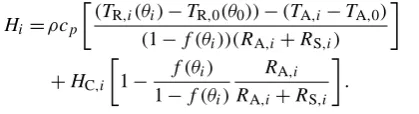
Hi =ρcp
(T
R,i(θ )−TR,0(θ ))−(TA,i−TA,0) (1−f (θ ))(RA,i+RS,i)
+HC,i
1− f (θ ) 1−f (θ )
RA,i RA,i+RS,i
+(H0−HC,0)
RA
,0+RS,0 RA,i+RS,i
+HC,0
f (θ ) 1−f (θ )
RA,0 RA,i+RS,i
. (5)
Since the first observation is taken to be at one hour past the sunrise, the soil sensible heat flux,HS,0=H0−HC,0, is
minimal and can be omitted. In practice HC,0 is also very
small so the last term is also omitted, thus avoiding the need to calculate any of the fluxes or resistances at timet0 and simplifying Eq. (5) to
Hi =ρcp
(TR
,i(θ )−TR,0(θ ))−(TA,i−TA,0) (1−f (θ ))(RA,i+RS,i)
+HC,i
1− f (θ ) 1−f (θ )
RA,i RA,i+RS,i
. (6)
In the original DTD model, ground heat flux,G, at time
ti was calculated as a fixed fraction (0.3) of the net
radia-tion reaching the soil, according to Eq. (9) in Norman et al.
(2000). In this study, we modelGaccording to the scheme proposed by Santanello and Friedl (2003), which, in addi-tion to the net radiaaddi-tion reaching the soil, takes into account the diurnal variation in surface radiometric temperature, as-sumed to be the difference between the LST observations at
ti andt0. Finally the total latent heat flux, LE, at timeti is
calculated as a residual of the other fluxes,
LEi=Rn,i−Gi−Hi, (7)
and the latent heat flux from the soil, LES, is also computed
as a residual:
LES=LE−LEC. (8)
2.2 Modifications to the effective Priestley–Taylor coefficient
In combination,αPTfgform an effective Priestley–Taylor co-efficient that is used to modify canopy transpiration rates computed, as in Eq. (4), from the divergence of net radia-tion within the canopy layer. Originally the DTD model was tested predominantly in rangelands and croplands during the growing season and before the onset of senescence (Norman et al., 2000). Under these conditions the model works quite well with the assumption that the vegetation is fully green (fg
set to a value of 1) and transpiring at the potential rate (αPT
initially set to the default value of 1.26, Priestley and Taylor, 1972). For canopies that are either stressed and not transpir-ing at the potential rate or are not fully green, modification to the effectiveαPTis required to yield reasonable partitioning between LECand LES. This can be accomplished by
modi-fying eitherαPTorfgor both parameters, as appropriate. In the TSEB, αPT is internally modified from its initial
value if the model results in negative values in the soil evap-oration rate, LES, given that condensation on the soil is
unlikely to occur during the day (Norman et al., 1995). If LES<0 is encountered, it is assumed that the canopy is
stressed and αPT is iteratively reduced until solutions with
LES>0 are obtained. This iterative scheme works well in
ecosystems where canopy values ofαPT are relatively
con-servative under unstressed conditions (Agam et al., 2010). For stressed canopies, the soil surface is usually dry and LES
close to zero is a reasonable assumption (Kustas and Ander-son, 2009). Unless additional information about phenologi-cal condition is available,fgis typically set to unity.
In this study a number of field validation sites are located in forested ecosystems. In forests, particularly in coniferous stands, observational studies find that unstressedαPT
associ-ated with canopy is significantly lower then typical value of 1.26 (Komatsu, 2005). As a result, settingfgto unity in the
DTD and downadjustingαPTiteratively from an initial value
of 1.26 can lead to overestimation of LE for these ecosys-tems.
One approach to addressing this issue in coniferous forests is to set the initialαPTbased on tree height,hC, as proposed by Komatsu (2005):
αPT= −0.371·ln(hC)+1.53. (9)
Equation (9) is derived empirically and takes into account a host of physiological influences on the vegetation transpi-ration, including the fraction of vegetation that is green and actively transpiring. Therefore adjustment tofg=1 is not necessary under this scheme. However this requires an es-timate ofhC, which is difficult to measure remotely in the absence of routine lidar datasets.
Another method might assumeαPT has a constant value based on an ecosystem type, which is then scaled to reflect current phenological conditions by adjustingfg. This method could be applicable not only in forests but also in grasslands and croplands during senescence. The fraction of vegetation that is green is set equal to the ratio of the fraction of pho-tosynthetically active radiation (PAR) absorbed by the green vegetation cover and fraction of PAR intercepted by the total vegetation cover, and can be estimated using vegetation in-dices (VIs). Specifically, Fisher et al. (2008) proposed using the normalized difference vegetation index (NDVI) and the enhanced vegetation index (EVI) to estimatefgas
fg=1.2
EVI
NDVI,0≤fg≤1. (10)
In this study, αPT for all ecosystems was given the initial value of 1.26. Green vegetation fraction was estimated at all sites using Eq. (10).
2.3 Adapting the DTD model for night-time LST observations
By exploiting the high temporal resolution of geostationary satellites, the original DTD model was able to set the first observation time,t0, at one hour past sunrise when fluxes
are minimal. This enabled the simplification of Eq. (5) into Eq. (6), thus avoiding the calculation of any fluxes or resis-tances at t0. Polar orbiting satellites do not have the tem-poral resolution of geostationary satellites. Terra and Aqua satellites used in combination provide 4 diurnal observations over most of the Earth’s land surface, with Terra overpasses around 10:30 and 22:30 local time (LT) and Aqua overpasses around 13:00 and 01:00 LT. During the growing season at high latitudes, 10:30 is well past sunrise and energy fluxes are already fully developed. Therefore, thet0time must be
associated with one of the night observations. In this study, the Aqua 01:00 LT overpass time was selected because it is closest to sunrise.
At night, energy fluxes are small but they are often larger than the early morning fluxes so they could potentially influ-ence the daytime flux estimation. During the 01:00 LT, Aqua overpass time there is no shortwave radiation component of
the net radiation. Therefore the Priestley–Taylor approxima-tion (Eq. 4) is not applicable for estimaapproxima-tion of canopy sen-sible heat flux. Instead it can be assumed that at night the temperature of the canopy,TC, is close to the in-canopy air
temperature,TAC, estimated by an extrapolation of the
dia-batic temperature profile, as described below. Then,TS can
be obtained by rearranging Eq. (1) and the sensible heat of both the canopy and soil,HC andHS respectively, can be
calculated from the basic TSEB equations (Norman et al., 1995):
HC=ρcp
TC−TA RA
(11)
HS=ρcp
TS−TA
RS+RA. (12)
Initially TCis set to the average of TRandTA and neu-tral atmospheric stability conditions are assumed (|L| → ∞). This allows for calculation of resistances as described in Sect. 2.1, except in this case without the Richardson num-ber approximation ofL. Once the resistances are known,H
can be calculated as the sum ofHCandHS.
It is not possible to use Eq. (8b) from Norman et al. (2000) to estimate 1Rn since it assumes solar radiation to be the
dominant component of the net radiation. Instead, the long-wave radiation divergences in the canopy,LN,C, and the soil, LN,S, are calculated according to Kustas and Norman (1999): LN,C=1−exp(κLF )]Lsky+LS−2LC (13) LN,S=exp(−κLF )Lsky+1−exp(−κLF )LC−LS, (14)
whereLsky,LSandLCare the long-wave emissions from the
sky, soil and vegetation canopy respectively.κLis the
extinc-tion coefficient for diffuse radiaextinc-tion in the canopy and is set to 0.95 for sparse vegetation (F <1) and to 0.7 for denser vegetation (Campbell and Norman, 1998). The total net ra-diation at night,Rn,0, is the sum ofLN,C0andLN,S0.Lskyis
calculated as described in Sect. 2.1, whileLSandLCare esti-mated using the Stefan Boltzman equation and the modelled soil and canopy surface temperatures. At night,Gcannot be estimated using the model proposed by Santanello and Friedl (2003), and instead a linear function of net radiation reaching the soil is used with the slope and intercept values of 0.3 and 35 W m−2respectively, chosen to be similar to values found
in other studies (Liebethal and Foken, 2007). LE is still cal-culated as the residual in the surface energy balance equation for the soil and canopy.
After obtaining the first estimates of H, the night-time canopy and soil surface temperatures can be recalculated. First, the equation for diabatic temperature profile in bound-ary layer is used (Campbell and Norman, 1998):
T (d0+z0H)=TA+ H
0.4ρcpu∗
lnzT−d0
z0H
+9H
vegetation height,d0is the zero plane displacement length,
z0H is roughness parameter for heat transfer and9H is the
Monin–Obukhov stability function for heat, calculated fol-lowing chapter 2.5 from Brutsaert (2005). Sinced0≈0.65hC
andz0H≈0.02hC(Norman et al., 2000), it can be assumed
that
TC≈TAC≈T (d0+z0H). (16)
This estimate ofTACusing Eq. (15) does not consider rough-ness sublayer effects on the temperature profile, as suggested by Harman and Finnigan (2008), but is considered a reason-able approximation for purposes of this study.u∗andLcan also be recalculated using the total latent and sensible heat fluxes, as described in Brutsaert (2005).
The above process is repeated until bothTC andL
con-verge to stable values. If concon-vergence is not obtained, all the fluxes are set to zero. In cases whereTAis less thanTR, the
fluxes are also set to zero since it is not physically plausible to have unstable atmospheric conditions over land surfaces at night. Most likely in such cases there are errors in theTR
retrieval.
If Eq. (5) is used with all the fluxes and resistances at timet0calculated as described above, then the t0 terms on the right-hand side of the equation cancel out and the model no longer utilizes the time-differential LST observations. To avoid this, at least one of the terms with fluxes calculated at time t0 needs to be assumed to be negligible and
re-moved from Eq. (5). Removing these terms could potentially increase the model error when significant night fluxes are present. However, it may also increase the robustness of the model when there is bias in the temperature data, the situa-tion that DTD was designed to address (Norman et al., 2000). In Sect. 4.1.2 we evaluate the impact of ignoring the night fluxes on the accuracy of the daytime estimates.
2.4 Additional considerations in using MODIS LST
When the model is driven by geostationary satellite data, the VZA remains constant between the two observations at times
t0andt1. This is not the case with polar satellites, as differ-ent overpasses follow differdiffer-ent orbital tracks and the VZA between the night and day observations changes. Therefore, Eq. (5) has to be modified slightly to take this into account:
Hi =ρcp
(T
R,i(θi)−TR,0(θ0))−(TA,i−TA,0) (1−f (θi))(RA,i+RS,i)
+HC,i
1− f (θi) 1−f (θi)
RA,i RA,i+RS,i
+(H0−HC,0)
1−
f (θ0)
1−f (θi)
RA,0+RS,0 RA,i+RS,i
+HC,0
f (θ0) 1−f (θi)
RA,0 RA,i+RS,i
, (17)
whereθ0is the VZA of the observation at timet0, andθi is
the VZA of the observation at timeti.
The MODIS LST V5 products (MOD11A1 for Terra and MYD11A1 for Aqua satellites) have been validated for a number of mostly homogeneous sites using both temperature-based and radiance-based methods, and in most cases RMSE has been within 1 K (Wan, 2008; Wan and Li, 2008; Coll et al., 2009). Wan (2008) validated MODIS LST over two lake sites and found that MODIS generally underes-timated the temperature during both day and night observa-tions and had a RMSE of 0.7 K. Wan and Li (2008) compared MODIS LST against radiance-based LST in playa, grass-land, lake and bare soil sites and found again that in most cases MODIS LST underestimates ground-based measure-ments, both during the day and night, and errors were usu-ally below 1 K, except for cases of bare soil where they were 1–2 K larger. Finally, Coll et al. (2009) looked at a rice field and a coniferous forest and observed an underestimation of MODIS LST of around−0.3 K with a RMSE of around 0.6 K at the rice field and negligible bias and a RMSE of 0.6 K at the forest site. The main identified causes of the underesti-mation bias were neglection of above-average atmospheric aerosol optical depths and difficulty in filtering out all cloud-affected observations, especially if the cloud cover was not very significant or consisted of cirrus clouds (Wan and Li, 2008). This problem is compounded at night, when it is more difficult to detect clouds (Neteler, 2010). The other identified sources of error were uncertainty in surface emissivities, es-pecially at the bare soil and heterogeneous sites (Wan and Li, 2008) and during the periods of high soil surface sur-face moisture, for example after rain events (Hulley et al., 2010). No correlation, however, was found between VZA or the satellite (Aqua or Terra) and the RMSE, and in general larger errors occurred during the day than at night (Wan and Li, 2008). The prevalent bias (underestimation) in both day and night LST retrievals present in the MODIS LST product would appear to make it highly suitable for application of the DTD approach.
3 Data
3.1 Danish field sites: HOBE
The Danish Hydrological ObsErvatory, HOBE, was estab-lished in 2007 to provide long-term datasets and environ-mental monitoring facilities for diverse hydrological studies (Jensen and Illangasekare, 2011). HOBE encompasses the Skjern River catchment on the western side of the Danish Jut-land peninsula and is located in the maritime climatic zone, with mild winters and cold summers, mean annual precip-itation of 990 mm and mean annual temperature of 8.2◦C. The catchment has an area of 2500 km2and is characterized by flat terrain, with the two main land uses being irrigated agriculture (68 % of the area) and forests (16 % of the area).
The two flux tower sites used for validation in this study are located in the Gludsted plantation forest (GLU) and
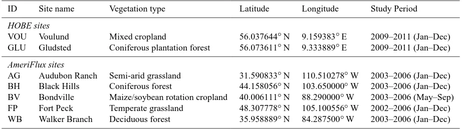
Table 1. List of flux towers providing the validation datasets used in this study. Information includes the ID and name of the flux tower, the
vegetation type in the vicinity of the tower, its location and the period of the data series used.
ID Site name Vegetation type Latitude Longitude Study Period
HOBE sites
VOU Voulund Mixed cropland 56.037644◦N 9.159383◦E 2009–2011 (Jan–Dec)
GLU Gludsted Coniferous plantation forest 56.073611◦N 9.333889◦E 2009–2011 (Jan–Dec)
AmeriFlux sites
AG Audubon Ranch Semi-arid grassland 31.590833◦N 110.510278◦W 2003–2006 (Jan–Dec)
BH Black Hills Coniferous forest 44.158056◦N 103.650000◦W 2003–2006 (Jan–Dec)
BV Bondville Maize/soybean rotation cropland 40.006111◦N 88.290000◦W 2003–2006 (May–Sep)
FP Fort Peck Temperate grassland 48.307778◦N 105.100556◦W 2002–2006 (Jan–Dec)
WB Walker Branch Deciduous forest 35.958889◦N 84.287500◦W 2003–2006 (Jan–Dec)
Voulund agricultural site (VOU) (Table 1). The Gludsted site is in the centre of a large homogeneous plantation domi-nated by 20 m tall Norway spruce (Picea abies). The eddy covariance (EC) equipment is mounted at a height of 37.5 m while the meteorological sensors are mounted 30 m above the ground. The flux measurements at GLU were collected throughout the whole of 2009, 2010 and 2011.
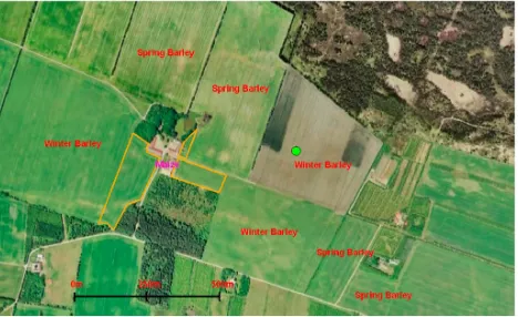
The Voulund site is much more heterogeneous (Fig. 1). The flux tower is surrounded by crop fields, with an average area of a couple of hectares, mostly sown with winter and summer varieties of barley and maize but also with potatoes and other crops. The EC system is mounted 6 m above the ground with the flux tower footprint covering several fields, mostly west of the tower, depending on wind speed and di-rection and stability. The MODIS pixel also covers a number of crop fields in addition to some adjacent forest groves. The fluxes at VOU were measured from 2009 through 2011. For more detailed description of the sites and the equipment used, the reader may refer to Ringgaard et al. (2011).
At both sites the fluxes and meteorological measurements were aggregated to 30 min intervals. Since DTD assumes that the incoming radiation is balanced by the outgoing en-ergy fluxes, this balance was enforced in cases where clo-sure was not achieved by assigning any residual energy (Rn−H−LE−G) to LE, following Prueger et al. (2005). Observations where LE became negative after being assigned the residual were removed from the analysis. In addition, any observations taken on days with snow cover or very little veg-etation (NDVI<0.25) were also removed.
As a baseline case, the model was also run using pre-dominantly ground-based measurements, with local LST es-timated from the upwelling long-wave radiation measured by pyrgeometers. However, due to technical problems, no such measurements were taken at GLU and so it is not possible to run the model with local LST observations at this site. There are no field-based LAI measurements taken at the HOBE sites so MODIS LAI, smoothed using TIMESAT (J¨onsson and Eklundh, 2004), was used as input into DTD.
3.2 AmeriFlux field sites
In addition to the Danish sites, a number of flux tower sites from the AmeriFlux network (http://public.ornl.gov/ ameriflux/) (Baldocchi et al., 2001) were also used to provide a more robust evaluation of model performance in different ecosystem types and climatic zones, even though these sites are at latitudes that are reasonably accommodated by geo-stationary satellites (Table 1). The Black Hills (BH) tower is situated in coniferous forest, Walker Branch (WB) is in a de-ciduous forest, Audubon Ranch (AG) is in semi-arid grass-land, Bondville (BV) is in rain-fed maize/soy bean crop-land and Fort Peck (FP) is in a temperate grasscrop-land. Appli-cation period depended on archive data availability at each site. For both local tests of the DTD model (driven by tower-based measurements of LST and LAI) and experiments us-ing MODIS-measured LST and LAI, the data from all the months of 2003 to 2006 (inclusive) have been used at BH, WB, AG sites, for 2002 to 2006 at FP, while at BV we used data from May till September for 2003 to 2006. The field measured data were 30 min averages, and energy balance clo-sure was enforced using the residual method applied to the HOBE datasets. Measurements over bare soil or snow cover were removed from the analysis based on the same criteria as for the HOBE dataset. For more details about the AmeriFlux sites used in this analysis, see Houborg et al. (2009).
3.3 MODIS products
Fig. 1. Orthophoto showing the heterogeneity of the Voulund
(VOU) field site. The labelled crop types were grown in 2009 and the green point indicates the location of the flux tower. Figure taken from Ringgaard et al. (2011).
relaxation of the cloudmask confidence threshold to define a pixel as clear-sky and the removal of temporal averaging to instead provide an instantaneous LST observations pro-jected on a Sinusoidal grid (Wan, 2008). The second refine-ment is particularly relevant in this case since it allows for comparison of the energy fluxes with tower based measure-ments taken simultaneously. Although the nominal resolu-tion of the product is 1 km by 1 km, the instantaneous field of view of the MODIS thermal-infrared sensor pixel is only that size when viewed from nadir and increases up to 2 km by 4.8 km at VZA of 60 degrees (Masuoka et al., 1998). This might be significant when evaluating modelled fluxes at het-erogeneous sites. Apart from the LST layer, the M*D11A1 (MYD11A1 and MOD11A1) products contain information about the time of the observation, the VZA, and quality flag, all of which are used in the algorithm, as well as emissiv-ity values which are needed to calculate the net long-wave radiation (see Sect. 2.1).
Another important model input parameter, used in par-titioning the radiometric surface temperature and modelled fluxes between canopy and soil, is the leaf area index (LAI), which comes from the MCD15A3 product (Knyazikhi et al., 1999). MCD15A3 provides LAI estimates at 4 day tempo-ral resolution utilizing observations from both the Terra and Aqua Satellites. The normalized difference vegetation index (NDVI) (Rouse et al., 1973) and enhanced vegetation index (EVI) (Gao et al., 2000) contained in the MOD13A2 Terra 16 day 1 km data product are used to estimate fraction of vegetation that is green as described in Sect. 2.2. Finally MCD43B3, an 8 day 1 km combined Terra and Aqua data product, is used to obtain an estimation of shortwave sur-face albedo, which is required to calculate the net shortwave radiation. To compute the actual surface albedo, MODIS-estimated black sky albedo (reflectance of direct beam ra-diation at solar noon) and white sky albedo (reflectance of isotropic diffuse radiation) products were combined based on
the ratio of downwelling direct and diffuse shortwave radia-tion, which under clear skies depends on the solar zenith an-gle and aerosol optical depth (Jin, 2003; Lucht et al., 2000). In this application of the DTD model, an assumption is made that on clear days around the solar noon, 80 % of reflected shortwave radiation comes from a direct beam and 20 % is diffuse, which is within the observed ranges (Roderick, 1999).
4 Results and discussion
4.1 Results using in situ data
4.1.1 Adjustingfgto improve modelling of canopy
heat fluxes
The effectiveness of modifyingfgto improve the accuracy of modelled fluxes was tested at all the field sites with the DTD driven by field based measurements (includingRn), with the
exception of NDVI and EVI used to computefg, which were
obtained from MODIS products. Since the LAI at the Amer-iFlux field sites is estimated as function of NDVI (Wilson and Meyers, 2007), it was assumed to quantify just the green part of the vegetation canopy (Houborg et al., 2009). How-ever, when calculating properties like radiation interception or wind profile in the canopy, the whole plant area index (or total LAI) should be used. Therefore the green LAI was divided byfg to obtain plant area index in cases when fg
was was less than unity; this was then used in all the DTD model equations. The same procedure was performed with the MODIS-derived LAI used at the VOU site. In the tests presented in this section, the first LST measurement was taken one hour past sunrise.
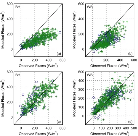
Figure 2 shows the effect of adjustingfgusing Eq. (10) on
sensible heat flux at a coniferous forest (BH) and a decidu-ous forest (WB), while Fig. 3 shows the effect at an agricul-tural site (VOU), temperate grassland (FP) and a semi-arid grassland (AG). At all the sites the fluxes are split into green growing season and senescence phases, which is assumed to begin when green LAI decreases by 20 % after reaching its peak. At some sites there is a large variability in the dates on which the transition from growing season to senescence happens in different years due to different crop types being grown, different climatological conditions and noise present in the LAI time series. These rough estimates are sufficient for the scope of this study, in which they are mostly used for presentation and analysis purposes. In all the cases when
fgwas set to unity (top panels), the sensible heat flux was
underestimated. At the forest sites there is no observable dif-ference between the bias in the sensible heat fluxes during growing season and senescent periods. However the differ-ence is very apparent at the grassland sites, with the sensible heat fluxes during senescence having a strong negative bias. At the agricultural site the senescence bias is less evident.
0 200 400 600 0
200 400 600
Observed Fluxes (W/m2)
Modeled Fluxes (W/m
2)
(a) BH
0 200 400 600 0
200 400 600
Observed Fluxes (W/m2)
Modeled Fluxes (W/m
2)
(b) WB
0 200 400 600 0
200 400 600
Observed Fluxes (W/m2)
Modeled Fluxes (W/m
2)
(c) BH
0 100 200 300 400 500 0
100 200 300 400 500
Observed Fluxes (W/m2)
Modeled Fluxes (W/m
2)
[image:8.595.52.285.61.291.2](d) WB
Fig. 2.Instantaneous modelled sensible heat flux during the growing season (crosses) and senescence (circles) with DTD driven by field measured LST witht0at one hour past sunrise at coniferous forest (BH,aandc) and deciduous forest (WB,bandd). At the top withfg= 1andαPT= 1.26for all vegetation types. At the bottom withfgadjusted based on MODIS VI. Senescence at BH starts between day of year (DOY) 142 and 359 and at WB between DOY 240 and 306.
27
Fig. 2. Instantaneous modelled sensible heat flux during the
grow-ing season (crosses) and senescence (circles) with DTD driven by field measured LST witht0at one hour past sunrise at coniferous
forest (BH, a and c) and deciduous forest (WB, b and d). The top panels – withfg=1 andαPT=1.26 for all vegetation types;
bot-tom panels – withfgadjusted based on MODIS VI. Senescence
at BH starts between day of year (DOY) 142 and 359 and at WB between DOY 240 and 306.
However after the VI-basedfgadjustment, the fluxes align along the 1–1 line, which is especially evident at the conif-erous forest site. Afterfgis adjusted, the bias inH at both the coniferous and deciduous forest sites (BH and WB re-spectively) becomes negligible. The growing-season bias at the grassland sites (FP and AG) is minimal and the bias dur-ing senescence is reduced but still significant after thefg
ad-justment (Table 2). This could be due to a scale mismatch between the local LAI observations and the 1 km scale fg
estimates, or the simple nature of thefgestimation scheme.
The only site where the error in the modelled sensible heat flux increases after thefgadjustment is the agricultural site, VOU, where the bias becomes positive but with a larger mag-nitude then whenfgwas kept at unity (Table 2).
To further explore the uncertainty introduced by the es-timation of fg from MODIS EVI and NDVI (fg,VI),
VI-based retrievals were compared withfg derived from field observations of LAI (fg, obs) at the BV agricultural site
(Fig. 4). To computefg, obs, it was assumed that at the
begin-ning of the growing season, the vegetation was fully green. After LAI reached its peak, total LAI was assumed con-served and the difference between the average peak LAI and observed LAI was converted to dead leaf area:fg, obs=
LAI/LAIpeak(Houborg et al., 2009). Although it is not likely
that LAI is conserved after reaching a peak value, since
during senescence leaves shrink/shrivel or fall off, this is con-sidered a first order approximation. During the beginning of the growing season,fg,VI shows only about 70 % of
vege-tation being green. At the peak of the growing season, both green fractions reach unity. The timing of the onset of senes-cence agrees between the field and satellite observations, but
fg, obsdrops to lower levels compared tofg,VI. The
discrep-ancies betweenfg,VIandfg, obshave a clear effect on the
es-timation of the sensible heat flux at BV. Figure 5b shows that the lower values offg,VIduring the beginning of the
grow-ing season cause overestimation ofH, while the higher val-ues offg,VIduring senescence cause underestimation ofH.
Whenfg, obs values are used, the bias during both the phe-nological stages is minimized (Fig. 5c). This suggests that the DTD may be used to estimate fluxes during senescence in grasslands and croplands as long as changes in the green vegetation fraction are reasonably accounted for.
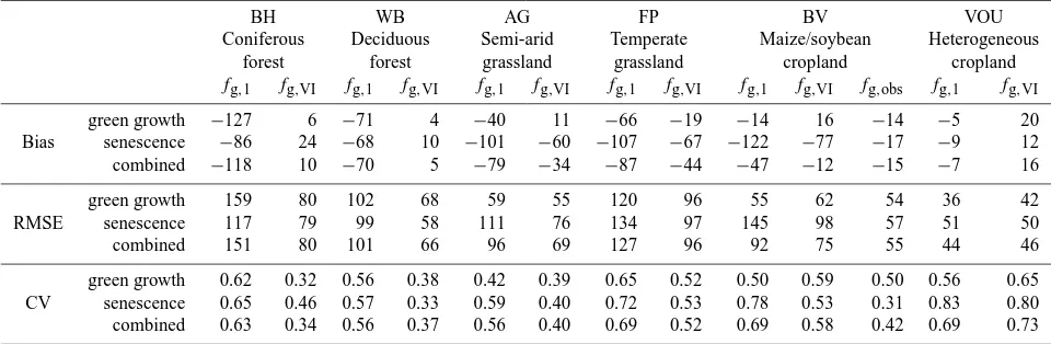
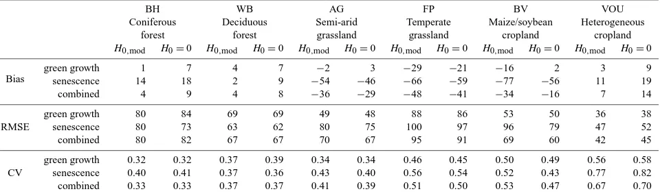
Table 2 demonstrates the impact on bias, root mean square error (RMSE) and the coefficient of variation of RMSE (de-fined as RMSE divided by the mean of the observed values, CV) as a result of modifying fg at all the validation sites.
Modifyingfgproduces, in most cases, substantial
improve-ment in the agreeimprove-ment between measured and modelledH. Since the total latent heat flux is calculated as a residual, sim-ilar improvement in LE is observed, disregarding errors in-troduced by the calculation ofG. The only exception is the increase in error at the agricultural sites during the growing season, whenfg,VI is less than one even though the crops
are fully green. However, the combined RMSE at BV is still significantly reduced since the magnitude ofH during the senescence is much larger than during the growing season and the reduction in error during senescence is also large. At VOU the error reduces marginally during senescence but not enough to compensate for the increase during the growing season, and the overall RMSE increases slightly.
To represent optimal model performance using only re-mote sensing inputs, all model runs presented in the fol-lowing sections used fg,VI. The only exception was at the
agricultural sites (BV and VOU) during the growing season, wherefgwas kept at unity to better reflect the actual state of
the crops.
4.1.2 Adjusting the model for night-time LST observations
In this section, we investigate the impact of using a first LST observation time,t0, in the DTD that occurs at night (01:30 LT), as in the case of MODIS applications. In these tests, nocturnal fluxes were either estimated with the model described in Sect. 2.3 or were assumed negligible as is the case in the original form of the DTD usingt0an hour after
Table 2. Bias (modelled−observed) and RMSE in W m−2and CV (unitless) of instantaneous modelled sensible heat flux at noon for fluxes during the growing season, senescence and the combined period, and usingfg=1 (fg,1), orfg adjusted based on VI (fg,VI), or based
on observations (fg, obs). Model runs usedt0at one hour after sunrise and were driven primarily by ground-based observations. MODIS
products were used to estimatefg,VIat all sites and LAI at VOU.
BH WB AG FP BV VOU
Coniferous Deciduous Semi-arid Temperate Maize/soybean Heterogeneous
forest forest grassland grassland cropland cropland
fg,1 fg,VI fg,1 fg,VI fg,1 fg,VI fg,1 fg,VI fg,1 fg,VI fg,obs fg,1 fg,VI
Bias
green growth −127 6 −71 4 −40 11 −66 −19 −14 16 −14 −5 20
senescence −86 24 −68 10 −101 −60 −107 −67 −122 −77 −17 −9 12 combined −118 10 −70 5 −79 −34 −87 −44 −47 −12 −15 −7 16
RMSE
green growth 159 80 102 68 59 55 120 96 55 62 54 36 42
senescence 117 79 99 58 111 76 134 97 145 98 57 51 50
combined 151 80 101 66 96 69 127 96 92 75 55 44 46
CV
green growth 0.62 0.32 0.56 0.38 0.42 0.39 0.65 0.52 0.50 0.59 0.50 0.56 0.65 senescence 0.65 0.46 0.57 0.33 0.59 0.40 0.72 0.53 0.78 0.53 0.31 0.83 0.80 combined 0.63 0.34 0.56 0.37 0.56 0.40 0.69 0.52 0.69 0.58 0.42 0.69 0.73
0 100 200 300 0
100 200 300
Observed Fluxes (W/m2)
Modeled Fluxes (W/m
2)
(a) VOU
0 200 400 600 0
200 400 600
Observed Fluxes (W/m2)
Modeled Fluxes (W/m
2)
(b) FP
0 100 200 300 0
100 200 300
Observed Fluxes (W/m2)
Modeled Fluxes (W/m
2)
(c) AG
0 100 200 300 0
100 200 300
Observed Fluxes (W/m2)
Modeled Fluxes (W/m
2)
(d) VOU
0 200 400 600 0
200 400 600
Observed Fluxes (W/m2)
Modeled Fluxes (W/m
2)
(e) FP
0 100 200 300 0
100 200 300
Observed Fluxes (W/m2)
Modeled Fluxes (W/m
2)
(f) AG
Fig. 3.Instantaneous modelled sensible heat flux during the growing season (crosses) and senescence (circles)
with DTD driven by field measured LST witht0at one hour past sunrise at agricultural site (VOU,aandd),
temperate grassland (FP,bande) and semi-arid grassland (AG,candf). At the top withfg= 1, at the bottom
withfgadjusted based on MODIS VI. Senescence at VOU starts between day of year (DOY) 175 and 215, at
FP between DOY 176 and 241 and at AG between DOY 239 and 261.
28
Fig. 3. Instantaneous modelled sensible heat flux during the growing season (crosses) and senescence (circles) with DTD driven by field
measured LST witht0at one hour past sunrise at agricultural site (VOU, a and d), temperate grassland (FP, b and e) and semi-arid grassland
(AG, c and f). The top panels – withfg=1; bottom panels – withfgadjusted based on MODIS VI. Senescence at VOU starts between day
of year (DOY) 175 and 215, at FP between DOY 176 and 241 and at AG between DOY 239 and 261.
AG, FP and VOU) and by over 50 % in the case of BH (by 23 W m−2). There is, however, negligible effect on RMSE at BV and an increase of almost 40 % at WB (by 10 W m−2), compared to the case when the nocturnal fluxes are assumed negligible.
However, using the nocturnal-flux estimates in the mod-elling of the day-time fluxes more often increases the dis-crepancies with the measurements. The 01:30 LT sensible
heat fluxes are predominantly negative and taking them into account in Eq. (5) reduces the estimated daytime sensible heat fluxHi. SinceHi is already frequently underestimated,
especially during senescence, taking the nocturnal fluxes into account actually increases the negative bias (underestimate) of the daytimeH (Table 3). The above is primarily a conse-quence of the model, and its input data, limitations and not a reflection of any underlying physical principle. However,
[image:9.595.110.482.234.532.2]Table 3. Bias (modelled−observed) and RMSE in W m−2and CV (unitless) of instantaneous modelled sensible heat flux at noon with the night-time sensible heat flux modelled (H0,mod) or assumed to be zero (H0=0). Model runs usedt0=01:30 LT and were driven primarily
by ground-based observations. MODIS products were used to estimatefg,VIat all sites and LAI at VOU.fg,VI=1 during green growth at
BV and VOU.
BH WB AG FP BV VOU
Coniferous Deciduous Semi-arid Temperate Maize/soybean Heterogeneous forest forest grassland grassland cropland cropland H0,mod H0=0 H0,mod H0=0 H0,mod H0=0 H0,mod H0=0 H0,mod H0=0 H0,mod H0=0
Bias
green growth 1 7 4 7 −2 3 −29 −21 −16 2 3 9 senescence 14 18 2 9 −54 −46 −66 −59 −77 −56 11 19 combined 4 9 4 8 −36 −29 −48 −41 −34 −16 7 14
RMSE
green growth 80 84 69 69 49 48 88 86 53 50 36 38 senescence 80 73 63 62 80 75 100 97 96 79 47 52 combined 80 82 67 67 70 67 95 91 69 60 42 45
CV
green growth 0.32 0.32 0.37 0.39 0.34 0.34 0.46 0.45 0.50 0.49 0.56 0.58 senescence 0.40 0.41 0.37 0.36 0.43 0.40 0.56 0.54 0.52 0.43 0.77 0.82 combined 0.33 0.33 0.37 0.37 0.41 0.39 0.51 0.50 0.53 0.47 0.67 0.70
2003 2004 2005 2006
0.1 0.2 0.3 0.4 0.5 0.6 0.7 0.8 0.9 1
Year
[image:10.595.51.287.266.523.2]Fraction of vegetation that is green
Fig. 4.Fraction of vegetation canopy that is green during the growing season at an agricultural site, BV. Solid line from field observations of LAI, broken line estimated using the VI method.
0 100 200 300 400 500
0 100 200 300 400 500
Observed Fluxes (W/m2)
Modeled Fluxes (W/m
2)
(a) BV
0 200 400 600
0 200 400 600
Observed Fluxes (W/m2)
Modeled Fluxes (W/m
2)
(b) BV
0 100 200 300 400 500
0 100 200 300 400 500
Observed Fluxes (W/m2)
Modeled Fluxes (W/m
2)
(c) BV
Fig. 5.Instantaneous modelled sensible heat flux during green growing season (crosses) and senescence (cir-cles) with DTD driven by field measured LST witht0at one hour past sunrise at the agricultural site (BV) with
fg= 1(a),fgadjusted based on VI(b)andfgfrom field observations of LAI(c). Senescence at BV starts between day of year 216 and 249.
Fig. 4. Fraction of vegetation canopy that is green during the
grow-ing season at an agricultural site, BV. Solid line from field observa-tions of LAI; broken line estimated using the VI method.
Table 3 also shows that even when nocturnal fluxes are ne-glected (H0=HC,0=0), the resulting accuracy is
compara-ble to that achieved when the first DTD observation is in the early morning. This is the case for both latent and sensible heat fluxes. Therefore, application of DTD using LST data collected from the night-time MODIS overpass fort0 does
not appear to cause significant errors in the computed day-timeHi.
We have also tested the robustness of the model when bias is introduced into the LST observations – a situation the DTD
technique was developed to address with its use of time-differential LST inputs. The model was run at the VOU site with both night-time and daytime LST offset by either±1◦C or ±5◦C to reflect moderate and extreme bias conditions, and with a night offset of −1◦C and day offset of−2◦C to approximate the expected bias conditions of MODIS LST (see Sect. 2.4). Several versions of Eq. (5) were used: (i) full Eq. (5); (ii) Eq. (5) withHC,0orHS,0omitted depending on
which one has a smaller magnitude; and (iii) bothHS,0and HC,0 omitted (Eq. 6). In all cases, night-time fluxes (HC,0
andHS,0) were modelled as described in Sect. 2.3. Table 4
shows that when no bias is introduced, the full form equation is the most accurate since it makes no assumption about night fluxes being insignificant; the other two versions of the equa-tion show a small increase in the model error. When positive bias is introduced, all the versions perform very similarly and revert to Eq. (6) in case of extreme positive bias sinceTR,0
becomes larger thanTA,0and the night-time fluxes are set to
zero (see Sect. 2.3). The biggest difference is when a neg-ative LST offset is introduced, although the RMSE remains relatively constant for the different model versions when run with moderate LST offset. The full form of Eq. (5) experi-ences the largest change in bias, as expected, since the mod-elled night fluxes are also biased and their inclusion in the model balances the reduction in error due to the use of time-differential LST. This is especially evident in the case of ex-treme negative LST offset. Equation (5) withHC,0 orHS,0
R. Guzinski et al.: Using two source energy balance model with day–night MODIS observations 2819
Table 4. RMSE and bias (modelled−observed) of instantaneous modelled energy fluxes (W m−2) for different model configurations. Driven by field data from Voulund, with and without bias introduced to both day (D) and night (N) LST measurements.
LST LST +1N/+1D LST +5N/+5D LST−1N/−1D LST−5N/−5D LST−1N/−2D RMSE Bias RMSE Bias RMSE Bias RMSE Bias RMSE Bias RMSE Bias
Eq. (5) 41 5 44 12 45 14 45 −8 81 −38 51 −25
Eq. (5),HC,0orHS,0omitted 42 7 44 13 45 14 45 −1 74 −32 48 −18 Eq. (5),HC,0andHS,0omitted 45 14 45 14 45 14 45 14 45 14 42 −4
2003
2004
2005
2006
0.1
0.2
0.3
0.4
0.5
0.6
0.7
0.8
0.9
Year
Fraction of vegetation that is green
Fig. 4.Fraction of vegetation canopy that is green during the growing season at an agricultural site, BV. Solid
line from field observations of LAI, broken line estimated using the VI method.
0 100 200 300 400 500 0
100 200 300 400 500
Observed Fluxes (W/m2)
Modeled Fluxes (W/m
2)
(a) BV
0 200 400 600 0
200 400 600
Observed Fluxes (W/m2)
Modeled Fluxes (W/m
2)
(b) BV
0 100 200 300 400 500 0
100 200 300 400 500
Observed Fluxes (W/m2)
Modeled Fluxes (W/m
2)
[image:11.595.51.550.96.157.2](c) BV
Fig. 5. Instantaneous modelled sensible heat flux during green growing season (crosses) and senescence
(cir-cles) with DTD driven by field measured LST witht0at one hour past sunrise at the agricultural site (BV) with
fg= 1(a),fgadjusted based on VI(b)andfgfrom field observations of LAI(c). Senescence at BV starts
between day of year 216 and 249.
[image:11.595.45.255.467.524.2]29
Fig. 5. Instantaneous modelled sensible heat flux during green growing season (crosses) and senescence (circles) with DTD driven by field
measured LST witht0at one hour past sunrise at the agricultural site (BV) withfg=1 (a),fgadjusted based on VI (b) andfgfrom field
observations of LAI (c). Senescence at BV starts between day of year 216 and 249.
In summary, using LST observations att0 occurring
dur-ing the night rather than in the early morndur-ing causes mini-mal degradation in the accuracy of DTD results, with some sites even showing improvement under this adjustment. This is true even when the night fluxes are assumed to be neg-ligible, and indicates that DTD can utilize night–day obser-vations. Therefore when using MODIS LST, the night-time fluxes can be ignored and Eq. (17) simplifies to:
Hi =ρcp
(T
R,i(θi)−TR,0(θ0))−(TA,i−TA,0) (1−f (θi))(RA,i+RS,i)
+HC,i
1− f (θi) 1−f (θi)
RA,i RA,i+RS,i
. (18)
4.2 Results using MODIS data
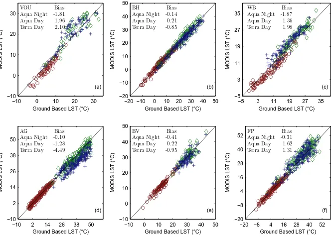
Previous studies have shown that MODIS LST estimates are often negatively biased with respect to ground-based obser-vations, for both night and day retrievals (Wan, 2008; Wan and Li, 2008; Coll et al., 2009). In this case, the use of a time-differential LST in the first term of Eq. (18) will reduce the impact of this bias on model estimates. However, this con-dition is not always met at the validation sites used in this study. Specifically, when comparing the LST measured us-ing ground instruments at the HOBE and AmeriFlux sites with the MODIS LST, the night-time MODIS LST is quently underestimated while daytime MODIS LST is fre-quently overestimated as shown in Fig. 6. The biases are par-ticularly large at VOU and WB, with FP and AG showing
negligible bias during the night but strong positive bias dur-ing the day. Applydur-ing Eq. (18) in those cases compounds the biases, and may increase model errors.
However, comparing MODIS derived LST to a single point-based measurement of LST is problematic for many landscapes due to the mismatch in the scale of the ground-based LST measurement and the MODIS LST pixel resolu-tion (Coll et al., 2009). This is especially evident during the day and could be the main cause of the observed bias mis-match between the night and day measurements. Since LST is a key input for the DTD model, this can lead to a large dis-crepancy between the measured and modelled energy fluxes. This is further complicated by an order of magnitude differ-ence between the source area contributing to the flux tower measurements (≈102×102m) and the area represented by the MODIS pixel (≈103×103m).
The DTD model, modified as described in Sect. 2 and us-ing Eq. (18), was run at the 7 validation sites usus-ing MODIS LST, LAI,fg, albedo and emissivities along with field
mea-surements of meteorological conditions (air temperature, rel-ative humidity, wind speed, pressure and incoming solar radi-ation) and vegetation height. Fluxes were modelled for a par-ticular day only if the night Aqua LST observation was of highest quality, as indicated by the quality flag, and at least one of the day Terra/Aqua LST observations was of highest quality as well. A statistical analysis comparing the instan-taneous modelled fluxes at timetiwith tower measurements is presented in Table 5, with scatter plots shown in Figs. 7 (forested sites), 8 (agricultural sites) and 9 (grassland sites).
2820 R. Guzinski et al.: Using two source energy balance model with day–night MODIS observations
−10 0 10 20 30
−10 0 10 20 30
Ground Based LST (°C)
MODIS LST (
°
C)
(a)
VOU Bias
Aqua Night -1.81
Aqua Day 1.96
Terra Day 2.10
−20 −10 0 10 20 30 40 50 −20 −10 0 10 20 30 40 50
Ground Based LST (°C)
MODIS LST (
°
C)
(b)
BH Bias
Aqua Night -0.14
Aqua Day 0.21
Terra Day -0.85
−5 3 11 19 27 35
−5 3 11 19 27 35
Ground Based LST (°C)
MODIS LST (
°
C)
(c)
WB Bias
Aqua Night -1.87
Aqua Day 1.36
Terra Day 1.98
−10 2 14 26 38 50 −10 2 14 26 38 50
Ground Based LST (°C)
MODIS LST (
°
C)
(d)
AG Bias
Aqua Night -0.10
Aqua Day -1.28
Terra Day -4.49
−10 0 10 20 30 40 50 −10 0 10 20 30 40 50
Ground Based LST (°C)
MODIS LST (
°
C)
(e)
BV Bias
Aqua Night -0.41
Aqua Day 0.22
Terra Day -0.95
−20 −8 4 16 28 40 52 −20 −8 4 16 28 40 52
Ground Based LST (°C)
MODIS LST (
°
C)
(f)
FP Bias
Aqua Night -0.31
Aqua Day 1.62
[image:12.595.133.467.64.302.2]Terra Day 1.31
Fig. 6. Comparison of ground measured LST with night time Aqua LST (circles), day time Aqua LST
(dia-monds) and day time Terra LST (crosses) at mixed crop land (VOU,a), coniferous forest(BH,b), deciduous
forest (WB,c), semi-arid grassland (AG,d), maize/soybean crop land (BV,e) and temperate grassland (FP,f).
Bias (MODIS LST – ground LST) is noted in◦C.
0 200 400 600 800 0
200 400 600 800
Observed Fluxes (W/m2)
Modeled Fluxes (W/m
2)
(a) GLU
0 200 400 600 800 0
200 400 600 800
Observed Fluxes (W/m2)
Modeled Fluxes (W/m
2)
(b) BH
0 200 400 600 800 0
200 400 600 800
Observed Fluxes (W/m2)
Modeled Fluxes (W/m
2)
(c) WB
Fig. 7.Instantaneous modelled net radiation (points), latent heat (diamonds), sensible heat (crosses) and ground
heat (x-es) fluxes at forested sites: coniferous (GLU,a), coniferous (BH,b) and deciduous (WB,c). DTD was
run using predominantly MODIS inputs withfgestimated using VI and night time fluxes ignored.
30
Fig. 6. Comparison of ground measured LST with night-time Aqua LST (circles), daytime Aqua LST (diamonds) and daytime Terra LST
(crosses) at mixed cropland (VOU, a), coniferous forest (BH, b), deciduous forest (WB, c), semi-arid grassland (AG, d), maize/soybean cropland (BV, e) and temperate grassland (FP, f). Bias (MODIS LST – ground LST) is noted in◦C.
−10 0 10 20 30
−10 0 10 20
Ground Based LST (°C)
MODIS LST (
°
C)
(a)
Aqua Day 1.96
Terra Day 2.10
−20 −10 0 10 20 30 40 50 −20 −10 0 10 20 30
Ground Based LST (°C)
MODIS LST (
°
C)
(b)
Aqua Day 0.21
Terra Day -0.85
−5 3 11 19 27 35
−5 3 11 19 27
Ground Based LST (°C)
MODIS LST (
°
C)
(c)
Aqua Day 1.36
Terra Day 1.98
−10 2 14 26 38 50 −10 2 14 26 38 50
Ground Based LST (°C)
MODIS LST (
°
C)
(d)
AG Bias
Aqua Night -0.10 Aqua Day -1.28 Terra Day -4.49
−10 0 10 20 30 40 50 −10 0 10 20 30 40 50
Ground Based LST (°C)
MODIS LST (
°
C)
(e)
BV Bias
Aqua Night -0.41
Aqua Day 0.22
Terra Day -0.95
−20 −8 4 16 28 40 52 −20 −8 4 16 28 40 52
Ground Based LST (°C)
MODIS LST (
°
C)
(f)
FP Bias
Aqua Night -0.31
Aqua Day 1.62
[image:12.595.130.465.362.473.2]Terra Day 1.31
Fig. 6. Comparison of ground measured LST with night time Aqua LST (circles), day time Aqua LST
(dia-monds) and day time Terra LST (crosses) at mixed crop land (VOU,a), coniferous forest(BH,b), deciduous
forest (WB,c), semi-arid grassland (AG,d), maize/soybean crop land (BV,e) and temperate grassland (FP,f).
Bias (MODIS LST – ground LST) is noted in◦C.
0 200 400 600 800 0
200 400 600 800
Observed Fluxes (W/m2)
Modeled Fluxes (W/m
2)
(a) GLU
0 200 400 600 800 0
200 400 600 800
Observed Fluxes (W/m2)
Modeled Fluxes (W/m
2)
(b) BH
0 200 400 600 800 0
200 400 600 800
Observed Fluxes (W/m2)
Modeled Fluxes (W/m
2)
(c) WB
Fig. 7.Instantaneous modelled net radiation (points), latent heat (diamonds), sensible heat (crosses) and ground
heat (x-es) fluxes at forested sites: coniferous (GLU,a), coniferous (BH,b) and deciduous (WB,c). DTD was
run using predominantly MODIS inputs withfgestimated using VI and night time fluxes ignored.
30
Fig. 7. Instantaneous modelled net radiation (points), latent heat (diamonds), sensible heat (crosses) and ground heat (x-es) fluxes at forested
sites: coniferous (GLU, a), coniferous (BH, b) and deciduous (WB, c). DTD was run using predominantly MODIS inputs, withfgestimated
using VI and night-time fluxes ignored.
The simpleRn estimation scheme in the DTD performs well at most sites, with the exception of semi-arid grassland (AG) where a large positive bias is present (Table 5). This is mostly caused by the underestimation in MODIS emissiv-ity at the predominantly bare soil site (results not shown) and may be improved in the upcoming V6 of the M*D11A1 prod-ucts (Wan, 2006). Further improvements can be expected by implementing the two-stream approach for estimating net ra-diation for soil and canopy (Kustas and Norman, 2000). Er-rors inGwere also acceptable (Table 5), especially within the context of the overall energy budget.
At most sites, the DTD performed well in partitioning the remaining available energy (Rn−G) between sensible and latent heat fluxes (Table 5) – particularly at the forested sites (Fig. 7). Partitioning was less accurate at the grassland sites,
AG and FP (Fig. 9), where strong positive bias in LE was observed, which may partly be caused by the relatively short period of vegetation activity, leading to low measured values of LE throughout most of the observation period. In addi-tion, the overestimation ofRn, particularly at AG, resulted in
overestimation of LE due to its calculation as residual. The presence of irrigated crops and a river within the FP MODIS pixel likely contributed to the overestimation of LE relative to the flux tower measurements.
0 200 400 600 0
200 400 600
Observed Fluxes (W/m2)
Modeled Fluxes (W/m
2)
(a) VOU
0 200 400 600 800 0
200 400 600 800
Observed Fluxes (W/m2)
Modeled Fluxes (W/m
2)
(b) BV
0 200 400 600 800 0
200 400 600 800
Observed Fluxes (W/m2)
Modeled Fluxes (W/m
2)
[image:13.595.130.465.65.174.2] [image:13.595.51.545.284.384.2](c) BV
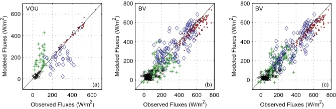
Fig. 8.Instantaneous modelled net radiation (points), latent heat (diamonds), sensible heat (crosses) and ground
heat (x-es) fluxes at crop land sites: mixed crops (VOU,a), maize/soybean rotation (BV,b), maize/soybean with
fgtaken from ground observations of LAI (BV,c). DTD was run using predominantly MODIS inputs with night
time fluxes ignored andfgin panels(a)and(b)estimated using VI during senscence and ketp at unity during
the growing season.
0 200 400 600 800 0
200 400 600 800
Observed Fluxes (W/m2)
Modeled Fluxes (W/m
2 )
(a) AG
0 200 400 600 0
200 400 600
Observed Fluxes (W/m2)
Modeled Fluxes (W/m
2 )
(b) FP
Fig. 9.Instantaneous modelled net radiation (points), latent heat (diamonds), sensible heat (crosses) and ground
heat (x-es) fluxes at grassland sites: AG semi-arid(a)and FP temperate(b). DTD was run using predominantly
MODIS inputs withfgestimated using VI and night time fluxes ignored.
[image:13.595.55.315.287.521.2]31
Fig. 8. Instantaneous modelled net radiation (points), latent heat (diamonds), sensible heat (crosses) and ground heat (x-es) fluxes at cropland
sites: mixed crops (VOU, a), maize/soybean rotation (BV, b), maize/soybean withfg taken from ground observations of LAI (BV, c).
DTD was run using predominantly MODIS inputs, with night-time fluxes ignored andfgin panels (a) and (b) estimated using VI during
senescence and kept at unity during the growing season.
Table 5. Comparison of modelled instantaneous daytime energy fluxes with flux tower measurements. RMSE and bias (modelled−observed) showed in W m−2, CV unitless. DTD was run using predominantly MODIS inputs, withfgestimated using VI, except at BV and VOU during
growing season wherefg=1, and night-time fluxes ignored.
Number of H LE Rn G
Site Ecosystem Observations Bias RMSE CV Bias RMSE CV Bias RMSE CV Bias RMSE CV GLU coniferous forest 34 51 97 0.34 −81 116 0.39 −34 37 0.06 −5 12 0.97 BH coniferous forest 121 −13 78 0.24 −12 78 0.29 −22 28 0.05 −2 20 0.91 WB deciduous forest 72 15 82 0.36 −34 93 0.23 −17 33 0.05 10 14 2.03 VOU heterogeneous cropland 37 93 122 1.43 −85 125 0.44 3 18 0.04 −12 19 0.47 BV maize/soybean cropland 105 −45 102 0.57 9 101 0.28 −44 63 0.11 −23 49 0.80 AG semi−arid grassland 281 −53 76 0.37 105 120 0.79 72 75 0.19 21 35 0.65 FP temperate grassland 162 −45 89 0.41 106 128 0.89 37 49 0.11 −38 54 0.54
0 200 400 600
0 200 400 600
Observed Fluxes (W/m2
)
Modeled Fluxes (W/m
2)
(a) VOU
0 200 400 600 800
0 200 400 600 800
Observed Fluxes (W/m2
)
Modeled Fluxes (W/m
2)
(b) BV
0 200 400 600 800
0 200 400 600 800
Observed Fluxes (W/m2
)
Modeled Fluxes (W/m
2)
[image:13.595.52.286.414.531.2](c) BV
Fig. 8.Instantaneous modelled net radiation (points), latent heat (diamonds), sensible heat (crosses) and ground heat (x-es) fluxes at crop land sites: mixed crops (VOU,a), maize/soybean rotation (BV,b), maize/soybean with fgtaken from ground observations of LAI (BV,c). DTD was run using predominantly MODIS inputs with night time fluxes ignored andfgin panels(a)and(b)estimated using VI during senscence and ketp at unity during the growing season.
0 200 400 600 800 0
200 400 600 800
Observed Fluxes (W/m2)
Modeled Fluxes (W/m
2)
(a) AG
0 200 400 600 0
200 400 600
Observed Fluxes (W/m2)
Modeled Fluxes (W/m
2)
(b) FP
Fig. 9.Instantaneous modelled net radiation (points), latent heat (diamonds), sensible heat (crosses) and ground heat (x-es) fluxes at grassland sites: AG semi-arid(a)and FP temperate(b). DTD was run using predominantly MODIS inputs withfgestimated using VI and night time fluxes ignored.
31
Fig. 9. Instantaneous modelled net radiation (points), latent heat
(di-amonds), sensible heat (crosses) and ground heat (x-es) fluxes at grassland sites: semi-arid (AG, a) and temperate (FP, b). DTD was run using predominantly MODIS inputs, withfgestimated using
VI and night-time fluxes ignored.
the errors are reduced (Fig. 8c). In particular, the RMSE ofH
reduces from 101 W m−2to 76 W m−2and the RMSE of LE reduces from 100 W m−2to 93 W m−2. Nevertheless, latent heat flux is modelled quite accurately during both crop peri-ods even when usingfg,VIduring senescence andfg=1
dur-ing growdur-ing season. At the VOU site, it should be noted that the MODIS-estimated LST exhibited strong negative bias at night and positive bias during the day when compared to
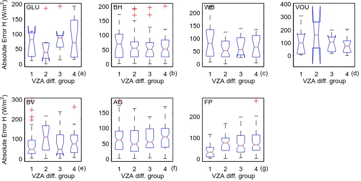
local ground-based measurements, which may contribute to overestimation of H and underestimation of LE by residual. The issue of inaccurate parametrization offg is most prob-ably present at this site as well, amplified by the different growing rates of the different ecosystems present within the MODIS pixel. Finally, the issue of sub-pixel heterogeneity is most problematic at this site – the tower is unlikely to be sam-pling fluxes that are representative at the 1 km scale (Fig. 1). We further investigated the impact of using the day and night LST observations with different VZA in Eq. (18) on the accuracy of the modelled fluxes. The sensible heat fluxes modelled with MODIS input data were grouped into four categories based onθdif= |θ1−θ0|: (1)θdif≤10, (2) 10< θdif≤20, (3) 20< θdif≤30, and (4)θdif>30. The
distribu-tion of absolute errors in each category was compared and the results are summarized in Fig. 10. The figure shows that there is no clear trend in the accuracy of the model asθdif
increases. At most of the sites there is no statistically signifi-cant difference at 5 % significance level between the medians of the absolute errors of the four categories, as indicated by the overlapping of the notched intervals. At the agricultural site BV and temperate grassland site FP, where there is sig-nificant difference between the median of the first category (with smallestθdif) and any of the other three categories, the first category has the smallest absolute errors. This indicates