Developing a decision support tool for assessing land use change and BMPs in ungauged watersheds based on decision rules provided by SWAT simulation

https://doi.org/10.5194/hess-22-3789-2018 © Author(s) 2018. This work is distributed under the Creative Commons Attribution 4.0 License.

Developing a decision support tool for assessing land

use change and BMPs in ungauged watersheds based

on decision rules provided by SWAT simulation

Junyu Qi1, Sheng Li2,3, Charles P.-A. Bourque2, Zisheng Xing2,4, and Fan-Rui Meng2

1_{Earth System Science Interdisciplinary Center, University of Maryland, College Park, 5825 University Research Ct,} College Park, MD, 20740, USA

2_{Faculty of Forestry and Environmental Management, University of New Brunswick, P.O. Box 44400, 28 Dineen Drive,} Fredericton, NB, E3B 5A3, Canada

3_{Potato Research Centre, Agriculture and Agri-Food Canada, P.O. Box 20280, 850 Lincoln Road,} Fredericton, NB, E3B 4Z7, Canada

4_{Portage La Prairie Site of Brandon Research and Development Centre, Agriculture and Agri-Food Canada, MB, Canada} Correspondence:Junyu Qi ([email protected])

Received: 15 July 2017 – Discussion started: 16 August 2017

Revised: 18 November 2017 – Accepted: 4 July 2018 – Published: 18 July 2018

Abstract.Decision making on water resources management at ungauged, especially large-scale watersheds relies on hy-drological modeling. Physically based distributed hydrolog-ical models require complicated setup, calibration, and val-idation processes, which may delay their acceptance among decision makers. This study presents an approach to develop a simple decision support tool (DST) for decision makers and economists to evaluate multiyear impacts of land use change and best management practices (BMPs) on water quantity and quality for ungauged watersheds. The example DST de-veloped in the present study was based on statistical equa-tions derived from Soil and Water Assessment Tool (SWAT) simulations and applied to a small experimental watershed in northwest New Brunswick. The DST was subsequently tested against field measurements and SWAT simulations for a larger watershed. Results from DST could reproduce both field data and model simulations of annual stream dis-charge and sediment and nutrient loadings. The relative er-ror of mean annual discharge and sediment, nitrate–nitrogen, and soluble-phosphorus loadings were −6, −52, 27, and −16 %, respectively, for long-term simulation. Compared with SWAT, DST has fewer input requirements and can be applied to multiple watersheds without additional calibra-tion. Also, scenario analyses with DST can be directly con-ducted for different combinations of land use and BMPs without complex model setup procedures. The approach in

developing DST can be applied to other regions of the world because of its flexible structure.

1 Introduction

Many studies have been conducted to evaluate the impact of land use change and BMPs on water quality based on field experiments (Novara et al., 2011; Pimentel and Krum-mel, 1987; Sadeghi et al., 2012; Turkelboom et al., 1997; Ur-bonas, 1994). Monitoring systems have been established to assess the impact of land use change and BMPs on water re-sources in order to capture the spatial and temporal variation in soil, climate, and topographic conditions in watersheds (Veldkamp and Lambin, 2001). Statistical models developed from field data from small watersheds are usually assumed to apply to large watersheds (Blöschl and Sivapalan, 1995; Blöschl and Grayson, 2001). Although it is not difficult to quantify soil erosion and chemical loadings in experimental plots, it is time-consuming and expensive (Mostaghimi et al., 1997). Clearly, it is not practical to conduct field experiments for every possible combination of land use and BMPs, under different biophysical conditions. As a result, it is unlikely sufficient field data could be obtained to develop manage-ment plans and conduct cost–benefit analyses. In addition, statistical models could potentially be derived from exper-iments; however, it is difficult to establish cause-and-effect relationships between BMPs and water quality variables un-der varied biophysical conditions or to quantify the impact of combined land use and BMPs on water quality at the water-shed scale (Renschler and Lee, 2005).

Process-based models of hydrology can be used to ex-trapolate field data to fill data gaps (Borah and Bera, 2003, 2004; Singh, 1995; Singh and Woolhiser, 2002; Singh and Frevert, 2005). These process-based models provide quanti-tative information that is usually difficult to obtain from field experiments (Borah et al., 2002). For example, ANSWERS (Beasley et al., 1980), CREAMS (Knisel, 1980), GLEAMS (Leonard et al., 1987), AGNPS (Young et al., 1989), EPIC (Sharpley and Williams, 1990), and the Soil and Water As-sessment Tool (SWAT; Arnold et al., 1998) have been used to understand surface runoff, soil erosion, nutrient leaching, and pollutant-transport processes. However, these process-based models require extensive input data and complex cal-ibration procedures (Liu et al., 2015); watersheds with suf-ficient data to calibrate and validate these models are nor-mally small, resulting in lack of representation at large spatial scales. Furthermore, once a model is calibrated, parameters become watershed-specific, which cannot be easily extended to other watersheds. In addition, these models require spe-cialized expertise, which prevents nonexpert decision makers and economists using them (Viavattene et al., 2008).

A decision support tool could be developed by combining “decision rules” with geographic information systems (GISs) for water quality assessment in large ungauged watersheds. The “decision rules” could be based on regression equa-tions derived from field experiments (Renschler and Harbor, 2002), or they could be defined simply as constants based on expert knowledge. Alternatively, simulations from a well-calibrated hydrological model could be used to develop sta-tistical equation-based “decision rules”. Apart from defining

“decision rules” at each grid cell, to assess water quantity and quality in streams or at subbasin and watershed outlets, the decision support tool should consider discharge, sedi-ment, and nutrient routing within the watershed. For exam-ple, a commonly used routing method for sediments is the sediment–delivery ratio (SDR) method, which is widely em-ployed in many GIS-based erosion models (May and Place, 2010; Wilson et al., 2001; Zhao et al., 2010). For discharge, a simple summation routing at the outlet produces accept-able accuracy for small- and medium-sized watersheds, con-sidering that there is negligible water losses from surface runoff and streamflow. For large watersheds, water losses are generally greater. These water losses can be estimated using simple linear equations. The annual export of nutrients from watersheds (via the nutrient–delivery ratio) has been stud-ied empirically in many studies as nutrient loading per land area (Endreny and Wood, 2003; Beaulac and Reckhow, 1982; Reckhow and Simpson, 1980).

A decision support tool developed based on “decision rules” is generally flexible and easy for decision makers and economists to use (Endreny and Wood, 2003). However, their practicality in normal circumstances, particularly with re-spect to their level of accuracy, needs to be evaluated. In addition, to provide sufficient “decision rules” with reason-able accuracy, fully validated hydrological models are re-quired to be able to fill data gaps in field experiments. The present study used SWAT to provide modeled data in the development of the decision support tool. The main objec-tive of the present study is to develop a simple decision sup-port tool with the intent to evaluate the impact of land use change and BMPs on water resources in a large ungauged watershed in New Brunswick, Canada. This paper presents the development and testing of a decision support tool us-ing data from two watersheds in the potato belt of New Brunswick: one small experimental watershed, with exten-sive monitoring and field survey data, and a larger watershed containing the smaller watershed. Specifically, this involves (1) setting up, calibrating, and validating SWAT for a small experimental watershed; (2) developing statistical equations relating water quality and quantity variables with weather, soil, land use information based on SWAT simulations for different combinations of land use and BMPs; (3) integrat-ing the statistical equations into a decision support tool with the aid of ArcGIS; and (4) testing the decision support tool against field measurements and model simulations of stream discharge, sediment, and nutrient loadings for a large water-shed.

2 Materials and methods

2.1 Study sites and data collection

Figure 1.Location of the Little River watershed (LRW) and Black Brook watershed (BBW) in New Brunswick (NB), Canada and water-monitoring stations no. 01 and no. 12 as well as weather stations no. 08 and St. Leonard. Elevations and subbasins are also shown for LRW.

of northwestern New Brunswick, Canada (Fig. 1). It covers an area approximately 380 km2 with a mixture of agricul-tural (16.2 %), forest (77 %), and residential (6.8 %) land uses (Xing et al., 2013). Elevation in the watershed ranges from 127 to 432 m a.m.s.l. (above mean sea level) (Fig. 1). The soil in the study sites is classified as mineral, derived from various parent materials. The major associations are Cari-bou, Carleton, Glassville, Grandfalls, Holmesville, McGee, Muniac, Siegas, Thibault, Undine, Victoria, Waasis, and one organic soil (Fig. 2). The study site belongs to the upper Saint John River valley ecoregion in the Atlantic Maritime Ecozone (Marshall et al., 1999). The climate of the region is considered to be moderately cool boreal with approxi-mately 120 frost-free days, annually (Yang et al., 2009). Daily maximum and minimum temperatures are 24 (in July) and−18.1◦C (in January) based on Canadian Climate Nor-mal station data at St. Leonard (http://climate.weather.gc.ca/ climate_normals, last access: 15 July 2018). The average temperature is 3.7◦C and annual precipitation is 1037.4 mm (Zhao et al., 2008). About one-third of the precipitation is in the form of snow. Snowmelt leads to major surface runoff and groundwater recharge events from March to May (Chow and Rees, 2006). The land use and soil maps in the setup of SWAT for LRW were derived from publicly available data (Department of Energy and Resource Development – ERD, New Brunswick; Fig. 2).

The small experimental watershed of the study is the Black Brook Watershed (BBW), a subbasin of LRW (Fig. 1). The BBW has been studied extensively for more than 20 years to evaluate the impact of agriculture on soil erosion and water quality (Li et al., 2014; Chow and Rees, 2006). The water-shed covers an area of 14.5 km2, with 65 % being

agricul-Figure 2.Slope classes created using a 10 m resolution lidar (light detection and ranging)-based DEM (digital elevation model), soil and land use maps, and land use IDs in SWAT (see Table 2 for land use ID meaning).

ture land, 21 % forest land, and 14 % residential areas and wetlands. Slopes vary from 1–6 % in the upper basin to 4– 9 % in the central area. In the lower portion of the water-shed, slopes are more strongly rolling at 5–16 %. Soil surveys (1:10 000 scale) identified six mineral soils, namely Grand-falls, Holmesville, Interval, Muniac, Siegas, and Undine, and one organic soil, St. Quentin (Mellerowicz, 1993).

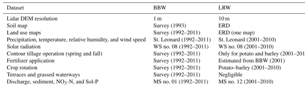
Table 1.Datasets in SWAT setup, calibration, and validation for BBW and LRW.

Dataset BBW LRW

Lidar DEM resolution 1 m 10 m

Soil map Survey (1993) ERD

Land use maps Survey (1992–2011) ERD (one map)

Precipitation, temperature, relative humidity, and wind speed St. Leonard (1992–2011) St. Leonard (2001–2010) Solar radiation WS no. 08 (1992–2011) WS no. 08 (2001–2010)

Contour tillage operation (spring and fall) Survey (1992–2011) Only for potato and barley (2001–2010) Fertilizer application Survey (1992–2011) Estimated from BBW (2001)

Crop rotation Survey (1992–2011) Potato–barley (2001–2010) Terraces and grassed waterways Survey (1992–2011) Negligible

Discharge, sediment, NO3-N, and Sol-P MS no. 01 (1992–2011) MS no. 12 (2001–2010)

Detailed description of data collection procedures and sam-ple analyses can be found in Chow et al. (2011). Weather data including daily precipitation, air temperature, relative humid-ity, and wind speed were acquired from the St. Leonard En-vironment Canada weather station (http://climate.weather.gc. ca, last access: 15 July 2018), located approximately 5 km northwest of BBW (Fig. 1). The daily average relative hu-midity and wind speed were calculated based on averaging hourly values. Since this weather station did not monitor daily solar radiation, the study used solar radiation collected from a weather station located approximately 10 km south-east of BBW (WS no. 08; Fig. 1).

2.2 SWAT setup, calibration, and validation for BBW and LRW

A modified version of SWAT has been developed for cold regions (Qi et al., 2016a, b, 2017a, b), and it was used for the BBW and LRW in this study. Detailed model setup, calibration, and validation for BBW can be found in Qi et al. (2017b). Specific model inputs for both watersheds are provided in Table 1. The same weather data were used for both watersheds (Table 1). The digital elevation model (DEM) for LRW and BBW were both based on high-resolution lidar (light detection and ranging) data; the first was created at 10 m and the second at 1 m resolution. The LRW was delineated into 32 subbasins from which their topographic characteristics were defined (Fig. 1). The soil types and slopes, which were classified into five separate classes, are illustrated in Fig. 2 for LRW. After combining the soil, slope, and land use maps through the ArcSWAT-interface function, 362 HRUs were subsequently created for LRW (based on thresholds: 10, 15, and 20 % for land use, soil, and slope).

Since only one land use map was available for LRW (Ta-ble 1), assumptions were made based on information avail-able on land use and management records for BBW to adjust the SWAT-management files for LRW as follows:

Table 2.Land use and land use groups for BBW and LRW.

Land use groups Land use ID Land use type in SWAT

General crops AGRL Agricultural land – generic

CANA Canola

CRON Corn

FPEA Field peas

POTA Potato

Grains BARL Barley

OATS Oats

PMIL Millet

RYE Rye

SWHT Spring wheat WWHT Winter wheat

Grasses BERM Bermuda grass

CLVR Clover

HAY Hay

PAST Past

RYEG Ryegrass

TIMO Timothy

Forestry FRSD Forest – deciduous

FRSE Forest – evergreen FRST Forest – mixed RNGB Range – bush WETF Wetlands – forested WETN∗ Wetlands – no forest Nonvegetated lands URMD Residential

UTRN Transportation UIDU∗ Industrial

Note: “∗_{” indicates unique land use types to LRW not present in BBW and, therefore,}

unaccounted for in the development of the decision support tool.

1. Potato–barley rotations were assigned to the land use ID POTA (Table 2); for other land use IDs, a single crop was considered.

fields over the entire watershed, based on 2001 survey data from BBW.

3. Contour tillage was applied only to potato and barley fields.

4. It was assumed that flow diversion terraces (FDTs) and grassed waterways in LRW were not used. It is worth noting that these four assumptions serve as a baseline scenario for the assessment of FDT in LRW.

To evaluate the global performance of the decision sup-port tool for LRW, related land use and management files were prepared and accessed by SWAT. For the purpose of comparison, simulations with SWAT were produced in an initial application by setting the adjustable parameters of the model to their default values, and in a second application by setting the parameters according to values produced with a watershed-specific model calibration to BBW. This approach with model parameterization is widely accepted when apply-ing SWAT to large ungauged watersheds (Panagopoulos et al., 2011).

2.3 Decision rules

The decision support tool was designed to use the “decision rules” to estimate annual discharge and sediment and nutrient loadings from individual grid cells:

A= n X

i=1

DRi·Ai, (1)

where A is the annual discharge or sediment and nutrient loadings at the outlet of the watershed, and DRi andAi are the delivery ratios and annual discharge or loadings, respec-tively, for grid celli. For the present study, statistical equa-tions derived from simulaequa-tions of the calibrated version of SWAT for BBW were defined as the “decision rules” in the decision support tool.

2.3.1 Land use groups and BMP scenarios

In statistical equation development, land uses in BBW (24, in total) were first classified into five land use groups according to their influences on hydrological processes (Table 2). Note that water land use type (WATR) was not used due to its small overall coverage (Fig. 2). As for watershed management, we considered three main BMPs, i.e.,

1. FDT+contour tillage, 2. contour tillage only, and

3. no-BMP (without FDT and contour tillage).

The calibrated version of the enhanced SWAT for BBW was used to generate annual outputs based on HRUs from 1992 to 2011. The model was run 3 times to generate the BMP-specific data for statistical equation development.

2.3.2 Explanatory variables selection

Explanatory candidate variables must be physically mean-ingful in hydrological and biochemical processes. It is worth noting that both continuous and categorical variables were included in the regression equation. The land use groups were the only categorical variable, and the remaining were all continuous variables. To detect significant predictors, the analysis of covariance (ANCOVA) was used. It requires at least one continuous and one categorical explanatory vari-able and is used to identify the major interaction of predictor variables. By including continuous variables, the method can reduce the variance of error to increase the statistical power and precision in estimating categorical variables (Keselman et al., 1998; Li et al., 2014). Inclusion of interaction terms in these regression models dramatically increased model per-formance.

In the present study, we only considered interactions be-tween two explanatory variables at a time. Student t tests were conducted to examine the statistical significance of each level of land use groups and their interaction with the vari-ous continuvari-ous variables. When one level of land use groups (e.g., grains; Table 2) did not significantly correlate with wa-ter quality or quantity, or there were nominal inwa-teractions between a given level and other explanatory variables, this particular level of land use groups would be combined with other levels of land use groups until all new levels of land use groups were statistically significant.

Multiple linear regression analyses were used to relate an-nual total discharge (mm) and sediment (t ha−1), NO3–N (kg ha−1), and Sol–P (kg ha−1) loadings to the explanatory variables. These work was conducted in R (Ihaka and Gen-tleman, 1996). Only six continuous explanatory variables were determined for the specification of the statistical mod-els. Annual precipitation (PCP), annual mean air tempera-ture (TMP), and mean saturated hydraulic conductivity of soil (SOL_K) were common to the dependent variables (i.e., total discharge and sediment, NO3–N, and Sol–P loadings). The LS factor (USLE_LS) and annual N and P application rates (N_APP and P_APP) were unique to the equations ad-dressing sediment, NO3–N, and Sol–P loading.

2.3.3 Delivery ratio definition

The LS factor of the universal soil loss equation (USLE) was determined by slope gradient (slp) and slope length (L) of individual HRUs:

USLE_LS= _L

22.1 m

·65.41·sin2(a)+4.56·sin(a)

+0.065) , (2)

wheremis the equation exponent anda is the angle of the slope (in degrees). The exponentmis calculated by

where slp is in units of meters per meter (m m−1). For the de-cision support tool, slope lengthLequal to the length of the grid side and slope gradient was determined by theSlopetool in ArcGIS. The sediment–delivery ratio was not considered in the decision support tool application to BBW. We assumed that annual sediment loadings from grid cells in the decision support tool were all exported to the outlet of BBW. How-ever, when the decision support tool was applied to LRW, the sediment–delivery ratio was used to correct estimates of sed-iment loading at the watershed outlet. The sedsed-iment loadings at the outlet of LRW (sed) were determined by

sed=SDR·sed∼, (4)

where sed∼_{is the sediment loading calculated with the}

sed-iment loading equation (one for each BMP and land use group), and SDR is determined by the following (Vanoni, 1975):

SDR=0.37·D−0.125, (5)

whereD(km−2) is the drainage area. For annual discharge and nutrient loadings, we assumed their delivery ratios are equal to 1.0 for all grid cells in LRW.

2.4 Decision support tool assessment

Inputs to the decision support tool included the six continu-ous explanatory variables and land use groups as well as in-formation on management practices, e.g., contour tillage and FDT implementation. Simulations from each grid cell were summarized at the outlet of the study watersheds. We first tested the impact of cell size on simulations of water quan-tity and quality at the outlet of BBW. The cell size range was determined by considering different farmland sizes in the watershed. We assumed that farmland-based grid cells can sufficiently represent basic hydrological processes, land use change, and management practice implementations for hy-drological modeling. Simulated annual water flow and sed-iment and nutrient loadings with the decision support tool were compared with those produced with the calibrated ver-sion of the enhanced SWAT. Subsequently, the deciver-sion sup-port tool was applied to LRW, and the simulations were com-pared with the results of the uncalibrated and calibrated ver-sions of SWAT. The purpose of this was to test if the decision support tool (i.e., land use and BMP assessment tool; LBAT) performed better, or at least as well, as both the uncalibrated and calibrated version of SWAT.

Model performance in terms of water quantity and quality at the outlet of the study watersheds was assessed based on the coefficient of determination (R2) and relative error (RE),

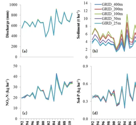
Figure 3.LBAT-produced simulations of annual stream discharge and sediment, NO3–N, and Sol–P loadings determined for different DEM grid-cell sizes (i.e., 25, 50, 100, 200, and 400 m).

i.e.,

R2= 

   

n P i=1

Oi−Oavg· Pi−Pavg

n P i=1

Oi−Oavg 2

· n P i=1

Pi−Pavg 20.5



    2

,

RE= Pavg−Oavg

Oavg

·100 %, (6)

whereOi,Pi,Oavg, andPavgare the observed and predicted and averages of the observed (O) and predicted (P) values. 2.5 FDT assessment in LRW

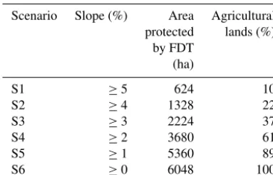
A series of FDT-implementation scenarios were set up for LBAT based on six slope classes to assess the impact of FDT on water quantity and quality on agricultural lands in LRW (Fig. 3; Table 3). From scenarios one (S1) to six (S6), the to-tal area protected by FDT gradually increased until all agri-cultural lands were protected (Table 3). Mean annual simu-lations of total discharge and sediment, NO3–N, and Sol–P loadings from LRW from 2001 to 2010 were compared with those of the baseline scenario (FDT=0 %) for each scenario using two performance indicators, i.e., mean difference (MD) and percentage relative difference (PRD), given as follows:

Table 3.Slope classes and corresponding areas in the agricultural land of LRW.

Scenario Slope (%) Area Agricultural protected lands (%)

by FDT (ha)

S1 ≥5 624 10

S2 ≥4 1328 22

S3 ≥3 2224 37

S4 ≥2 3680 61

S5 ≥1 5360 89

S6 ≥0 6048 100

3 Results and discussion

3.1 Statistical equations (decision rules) 3.1.1 Model structure and coefficients

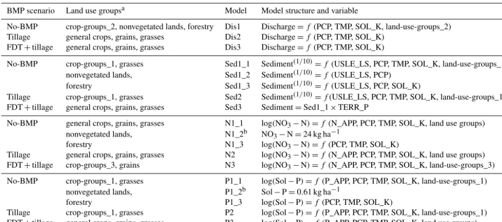
Linear regression equations and their explanatory variables for annual discharge and sediment, NO3–N, and Sol–P load-ings under different combinations of land use groups and BMP scenarios are provided in Tables 4 and 5. In total, three discharge models (Dis1, Dis2, and Dis3) and five sediment (Sed1_1, Sed1_2, Sed1_3, Sed2, and Sed3), NO3–N (N1_1, N1_2, N1_3, N2, and N3), and Sol–P (P1_1, P1_2, P1_3, P2, and P3) loading models were developed. Data transfor-mations (via logarithm and power transfortransfor-mations) were ap-plied to sediment, NO3–N, and Sol–P loadings to meet the assumption of normality in multiple regression analysis (Ta-ble 4). The contour tillage and FDT were applied only to agri-cultural lands (including general crops, grains, and grasses; Table 4). For the no-BMP scenario, three separate sediment, NO3–N, and Sol–P loading models were developed for agri-cultural lands, nonvegetated lands, and forestry, and one dis-charge model (Dis1) for all land use groups (Table 4). It is worth noting that the sediment loading model, Sed3, was a modified version of Sed1_1 (multiplied by TERR_P) for the FDT+contour tillage scenario (Table 4), and the values of TERR_P (Qi et al., 2017b) used for Sed3 were the same as the calibrated values in SWAT for BBW (Qi et al., 2017b). Also, NO3–N and Sol–P loadings (N1_2 and P1_2) for non-vegetated lands were determined as constants, which were equal to the calculated means of NO3–N and Sol–P loadings determined by SWAT (i.e., 24 and 0.61 kg ha−1_{, respectively;} Table 4).

In model development, three new land use groups (i.e., groups_1, groups_2, and land-use-groups_3) were formulated by combining general crops, grains, and grasses (Tables 4 and 5). For example, land-use-groups_2 was derived by combining general crops, grains, and grasses on total discharge (i.e., Dis1 model). Individ-ual model structures are shown in Table 4, whereas the

ex-planatory variables for these models appear in Appendix A. The coefficients estimated for the explanatory variables and their interactions, and theirt-test results are also shown in Appendix A. Most of the p values for these explanatory variables were <0.001, except for several that were be-tween 0.001 and 0.08, which were also taken as acceptable. 3.1.2 Statistical equation assessment

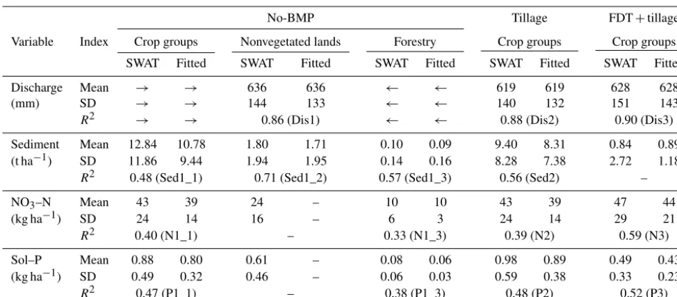
Simulations based on the statistical equations and the calcu-lated outputs from individual HRUs for the different BMPs are compared in Table 6. In general, discharge models were able to reproduce SWAT simulations for the three BMPs, with R2 ranging from 0.86 to 0.9. Mean discharge sim-ulated with the statistical equations was equal to that of SWAT (Table 6). Mean discharge (636 mm) for the no-BMP-case (BMP 3) was greater than that for BMPs using contour tillage and FDTs (619 and 628 mm for BMP 1 and 2, respec-tively), suggesting that contour tillage and FDTs can cause evapotranspiration to increase.

Models Sed1_2 and Sed1_3 were able to reproduce sim-ulations with SWAT (yieldingR2=0.71 and 0.57, respec-tively), and simulated mean sediment loadings were close to that of SWAT (Table 6). Models Sed1_1 and Sed2 tended to underestimate results from SWAT (Table 6), with an overall lower mean sediment loading of 10.78 vs. 12.84 and 8.31 vs. 9.4 t ha−1, respectively. Mean sediment load-ing with Sed3 (0.89 t ha−1) was slightly greater than that of SWAT (0.84 t ha−1), because Sed3 only took into account TERR_P, whereas SWAT took into account TERR_CN and the impact of grassed waterways. Results from the statistical equations showed that the mean sediment loading for BMP 2 (8.31 t ha−1_{) was significantly different than that for BMPs 1} and 3, with mean loading of 0.89 and 10.78 t ha−1(Table 6). The smallest mean sediment loading (0.09 t ha−1) was found to occur with the forestry land use grouping (Table 6).

load-Figure 4.Impact of grid-cell size on LBAT simulation of sediment loading. Mean annual sediment loadings and standard errors (verti-cal bars) from 1992 to 2011 are indicated.

ings for the forestry land grouping (10 vs. 0.06 kg ha−1_{) were} much less than those of the crop groups (including general crops, grains, and grasses), 39 vs. 0.8 kg ha−1(Table 6). 3.2 LBAT assessment

3.2.1 Impact of grid cell size on LBAT simulation Simulations of water quantity and quality by LBAT with different grid-cell sizes (i.e., 25, 50, 100, 200, and 400 m) for BBW are shown in Fig. 3. Statistical tests indicated that grid-cell size had a significant effect on sediment load-ing (pvalue<0.01), with no effect observed for discharge and NO3–N and Sol–P loadings (pvalues>0.99). Increas-ing cell size (i.e., slope length) increased sediment loadIncreas-ing. However, the mean slope gradient was reduced. As a result, the mean sediment loadings were correlated nonlinearly with cell size, as shown in Fig. 4. The highest mean sediment load-ing was found with a cell size of 100 m (5.86 t ha−1), whereas the lowest was found to occur with a cell size of 25 and 400 m (3.37 t ha−1). The LBAT with a cell size of 25 and 400 m was able to generate sediment loadings consistent with field mea-surements. Considering computational efficiency, we chose a grid-cell size of 400 m as the basic LBAT-simulation unit for LRW.

3.2.2 LBAT vs. SWAT in LRW

Simulations of water quantity and quality with LBAT and the uncalibrated and calibrated versions of SWAT are compared with field measurements for LRW (Fig. 5). Model assess-ments for different simulation periods (depending on mea-surement availability) are shown in Table 7. It is worth not-ing that, to eliminate unrealistic results, USLE_LS was con-strained in Sed1_2 to the nonvegetated lands:

USLE_LS=

Eq. (2) USLE_LS≤1.28,

1.28 USLE_LS>1.28, (7)

where 1.28 is the maximum USLE_LS for BBW.

Figure 5. Simulations of annual stream discharge and sediment, NO₃–N, and Sol–P loadings with LBAT and SWAT compared with field measurements at the outlet of LRW.

Table 4.Statistical models based on land use groups and BMP scenarios.

BMP scenario Land use groupsa Model Model structure and variable

No-BMP crop-groups_2, nonvegetated lands, forestry Dis1 Discharge=f(PCP, TMP, SOL_K, land-use-groups_2) Tillage general crops, grains, grasses Dis2 Discharge=f(PCP, TMP, SOL_K)

FDT+tillage general crops, grains, grasses Dis3 Discharge=f(PCP, TMP, SOL_K)

No-BMP crop-groups_1, grasses Sed1_1 Sediment(1/10)=f (USLE_LS, PCP, TMP, SOL_K, land-use-groups_1) nonvegetated lands, Sed1_2 Sediment(1/10)=f (USLE_LS, PCP)

forestry Sed1_3 Sediment(1/10)=f (USLE_LS, PCP, SOL_K)

Tillage crop-groups_1, grasses Sed2 Sediment(1/10)=f(USLE_LS, PCP, TMP, SOL_K, land-use-groups_1) FDT+tillage general crops, grains, grasses Sed3 Sediment=Sed1_1×TERR_P

No-BMP general crops, grains, grasses N1_1 log(NO3−N)=f(N_APP, PCP, TMP, SOL_K, land use groups) nonvegetated lands, N1_2b NO3−N=24 kg ha−1

forestry N1_3 log(NO3−N)=f(PCP, TMP, SOL_K)

Tillage general crops, grains, grasses N2 log(NO3−N)=f(N_APP, PCP, TMP, SOL_K, land use groups) FDT+tillage crop-groups_3, grains N3 log(NO3−N)=f(N_APP, PCP, TMP, SOL_K, land-use-groups_3) No-BMP crop-groups_1, grasses P1_1 log(Sol−P)=f(P_APP, PCP, TMP, SOL_K, land-use-groups_1)

nonvegetated lands, P1_2b Sol−P=0.61 kg ha−1

forestry P1_3 log(Sol−P)=f(PCP, TMP, SOL_K)

Tillage crop-groups_1, grasses P2 log(Sol−P)=f(P_APP, PCP, TMP, SOL_K, land-use-groups_1) FDT+tillage general crops, grains, grasses P3 log(Sol−P)=f(P_APP, PCP, TMP, SOL_K, land use groups)

a_{General crops and grains are combined into one group, namely crop-groups_1 in land-use-groups_1; general crops, grains, and grasses are combined into one group, namely crop-groups_2 in}

land-use-groups_2; general crops and grasses are combined into one group, namely crop-groups_3 in land-use-groups_3.b_{Variable is set constant.}

Table 5.Explanatory variables determined for statistical analysis.

Variable Unit Meaning

land use groups – Including general crops, grains, grasses, forestry, and nonvegetated lands land-use-groups_1 – General crops and grains are combined into a new group: crop-groups_1 land-use-groups_2 – General crops, grains, and grasses are combined into a new group: crop-groups_2 land-use-groups_3 – General crops and grasses are combined into a new group: crop-groups_3 N_APP kg ha−1 Annual N application rate

P_APP kg ha−1 Annual P application rate PCP mm Annual precipitation

SOL_K mm h−1 Mean saturated hydraulic conductivity of soil TERR_P – P factor for FDT

TMP ◦ Annual mean air temperature USLE_LS – LS factor of USLE

and d). The LBAT had the smallest absolute value of RE (i.e., RE= −16), while the uncalibrated and calibrated versions of SWAT had larger values (RE= −59 and−55, respectively). These results suggested that the LBAT and the calibrated version of SWAT performed fairly equivalently in simulat-ing annual streamflow and sediment and NO3–N loadings, with LBAT performing slightly better for annual Sol–P load-ing. LBAT performed noticeably better than the uncalibrated version of SWAT, especially for annual sediment and NO3– N loadings. Poor performance for both versions of SWAT and LBAT on simulation of annual sediment and Sol–P load-ings in LRW might be attributable to a lack of detailed man-agement practice and fertilizer application information from agricultural lands. We only had 1 year of data for LRW and made assumptions about rotation and management practices

for other years based on information from BBW, which could introduce major input uncertainty.

Since LBAT is based on decision rules (statistical equa-tions in this study) that were derived from SWAT simulaequa-tions for BBW, its usage should be constrained to areas with soil, landscape, and land use characteristics similar to BBW. Input characteristics exceeding the range of SWAT data could lead to large errors in predictions. LBAT is flexible in its structure, and with thoughtful development of decision rules, it can be applied to diverse environments.

3.2.3 FDT assessment in LRW

Table 6.Comparisons of simulations of statistical models and outputs from SWAT for different land use groups and BMPs based on mean and standard deviation for the entire simulation period (1992–2011).

No-BMP Tillage FDT+tillage

Variable Index Crop groups Nonvegetated lands Forestry Crop groups Crop groups

SWAT Fitted SWAT Fitted SWAT Fitted SWAT Fitted SWAT Fitted

Discharge Mean → → 636 636 ← ← 619 619 628 628

(mm) SD → → 144 133 ← ← 140 132 151 143

R2 → → 0.86 (Dis1) ← ← 0.88 (Dis2) 0.90 (Dis3) Sediment Mean 12.84 10.78 1.80 1.71 0.10 0.09 9.40 8.31 0.84 0.89 (t ha−1) SD 11.86 9.44 1.94 1.95 0.14 0.16 8.28 7.38 2.72 1.18

R2 0.48 (Sed1_1) 0.71 (Sed1_2) 0.57 (Sed1_3) 0.56 (Sed2) –

NO3–N Mean 43 39 24 – 10 10 43 39 47 44

(kg ha−1) SD 24 14 16 – 6 3 24 14 29 21

R2 0.40 (N1_1) – 0.33 (N1_3) 0.39 (N2) 0.59 (N3) Sol–P Mean 0.88 0.80 0.61 – 0.08 0.06 0.98 0.89 0.49 0.43 (kg ha−1) SD 0.49 0.32 0.46 – 0.06 0.03 0.59 0.38 0.33 0.23

R2 0.47 (P1_1) – 0.38 (P1_3) 0.48 (P2) 0.52 (P3)

Note: crop groups include general crops, grains, and grasses; the statistics for discharge in no-BMP scenario are based on crop groups, nonvegetated lands, and forestry.

Table 7.Statistical assessments of LBAT and SWAT for annual stream discharge and sediment, NO3–N, and Sol–P loadings at the outlet of LRW for different simulation periods.

Period Variable Index Measurement SWAT- SWAT- LBAT uncalibrated calibrated

01–07 Discharge Mean 704 691 638 664

(mm) RE (%) – −2 −9 −6

R2 – 0.63 0.69 0.54

01–10 Sediment Mean 0.95 2.95 0.65 0.45 (t ha−1) RE (%) – 212 −32 −52

R2 – 0.01 0.01 0.04

03–10 NO3–N Mean 12 22 14 15 (kg ha−1) RE (%) – 87 22 27

R2 – 0.59 0.45 0.35

03–10 Sol–P Mean 0.31 0.13 0.14 0.26 (kg ha−1) RE (%) – −59 −55 −16

R2 – 0.02 0.11 0.01

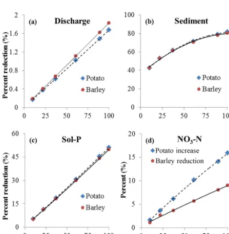
626 mm greater than that for the six FDT scenarios (Table 8). When all agricultural lands were protected (S6), there was a 2 % reduction in discharge (equivalent to 11 mm; Table 8). With the steepest areas protected (accounting for 10 % of the total land base; S1), the mean annual sediment loading was reduced by as much as 43 % (equivalent to 4.5 t ha−1; Ta-ble 8) and by as much as 81 % (i.e., 8.57 t ha−1) with all agri-cultural lands protected (S6; Table 8). Mean annual Sol–P loading was reduced by 51 % (equivalent to 0.47 kg ha−1; Ta-ble 8). In contrast, increased usage of FDT tended to increase

the mean annual loading of NO3–N by about 6 % when used across all agricultural lands (equivalent to 1.73 kg ha−1).

in-Table 8.Impact of FDT on mean annual discharge and sediment, NO₃–N, and Sol–P loadings simulated with LBAT under different FDT, provided in Table 3.

Variable Index Baseline S1 S2 S3 S4 S5 S6

Discharge Mean 626 625 623 622 619 616 615 (mm) MD – −1 −2 −4 −7 −10 −11 PRD (%) – 0 0 −1 −1 −2 −2

Sediment Mean 10.54 6.04 4.94 4.02 3.04 2.26 1.97 (t ha−1) MD – −4.50 −5.60 −6.52 −7.50 −8.28 −8.57 PRD (%) – −43 −53 −62 −71 −79 −81

NO3–N Mean 29.70 29.86 30.02 30.34 30.82 31.22 31.42 (kg ha−1) MD – 0.16 0.32 0.64 1.13 1.52 1.73

PRD (%) – 1 1 2 4 5 6

Sol–P Mean 0.94 0.89 0.83 0.76 0.65 0.52 0.46 (kg ha−1) MD – −0.05 −0.11 −0.17 −0.28 −0.42 −0.47 PRD (%) – −5 −11 −19 −30 −45 −51

Figure 6.Percentage change in discharge and sediment, NO3–N, and Sol–P loadings as a function of % area, where FDTs were used.

creased linearly for potato, while it decreased for barley. The increase for potato was nearly twice as much as the reduc-tion for barley (Fig. 6d). Seemingly the interacreduc-tion between barley and FDT had positive impacts on nitrate retention in soils, whereas the interaction between potato and FDT had an opposite effect.

These results are consistent with the results from previous studies (Yang et al., 2010, 2012), which used SWAT to as-sess the impact of FDT on water quantity and quality within BBW. When using SWAT, greater efforts are needed to pre-pare basic inputs, such as daily weather records, to proceed

with its calibration and validation, involving complex sce-nario setup and analysis. For every new watershed, SWAT needs dedicated effort and time for its setup. LBAT, in con-trast, can be used for multiple watersheds as long as they have similar environmental conditions. Scenario analysis can be directly conducted with different combinations of land use and BMPs using fewer inputs than what is required by SWAT. Also, once developed, LBAT does not require additional cal-ibration.

4 Conclusion

The present study addresses the development of a decision support tool to assess the impact of land use change and BMPs on water quantity and quality for ungauged water-sheds. An enhanced version of SWAT was calibrated and validated for a small experimental watershed. Multiple re-gression analyses were used to develop statistical equations based on simulations from SWAT. In total, three discharge and five sediment, NO3–N, and Sol–P loading models were developed for different combinations of land use groups and BMP scenarios. Only four common predictors (i.e., annual precipitation, annual mean air temperature, mean saturated hydraulic conductivity of soil, and land use groups) and three unique predictors (LS factor and annual nitrogen and phos-phorus application rates for sediment, NO3–N, and Sol–P loading models, respectively) are required.

equiv-alently with respect to annual stream discharge and sediment and NO3–N loadings. LBAT performed slightly better, when Sol–P loading was considered. Compared with the uncali-brated version of SWAT, LBAT performed better. The im-pact of FDT on water quantity and quality was evaluated with LBAT for LRW; its results were consistent with the re-sults generated with SWAT for the same region in previous studies. LBAT has fewer input requirements than SWAT and can be applied to multiple watersheds without additional cal-ibration. Also, scenario analyses can be directly conducted with LBAT without complex setup procedures. We recom-mend using LBAT for economic analysis and management decision making for watersheds with similar environmental conditions of New Brunswick. The LBAT developed in this study may not be directly applied to other regions; however, the approach in developing LBAT can be applied to other re-gions of the world because of its flexible structure.

Appendix A

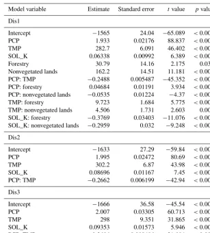
Table A1.Coefficient values for the three discharge models.

Model variable Estimate Standard error tvalue pvalue

Dis1

Intercept −1565 24.04 −65.089 <0.001 PCP 1.933 0.02176 88.837 <0.001 TMP 282.7 6.091 46.402 <0.001 SOL_K 0.06338 0.00992 6.389 <0.001 Forestry 30.79 14.16 2.175 0.030 Nonvegetated lands 162.2 14.51 11.181 <0.001 PCP: TMP −0.2488 0.005487 −45.352 <0.001 PCP: forestry 0.04684 0.01191 3.934 <0.001 PCP: nonvegetated lands −0.0535 0.01224 −4.37 <0.001 TMP: forestry 9.723 1.684 5.775 <0.001 TMP: nonvegetated lands 4.506 1.731 2.603 0.009 SOL_K: forestry −0.3769 0.03403 −11.076 <0.001 SOL_K: nonvegetated lands −0.2959 0.032 −9.248 <0.001

Dis2

Intercept −1633 27.29 −59.84 <0.001 PCP 1.995 0.02472 80.69 <0.001 TMP 302.2 6.87 43.98 <0.001 SOL_K 0.08696 0.01167 7.45 <0.001 PCP: TMP −0.2662 0.006199 −42.94 <0.001

Dis3

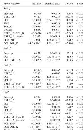
Table A2.Coefficient values for the four sediment loading models.

Model variable Estimate Standard error tvalue pvalue

Sed1_1

Intercept 0.2749 0.06125 4.488 <0.001 USLE_LS 0.1201 0.02224 54.018 <0.001 PCP 0.000788 5.54×10−5 14.218 <0.001 TMP 0.1117 0.01528 7.307 <0.001 SOL_K 0.000568 0.00022 2.585 0.010 Grasses −0.0353 0.00881 −4.007 <0.001 USLE_LS: SOL_K −0.00014 4.69×10−5 −3.045 0.002 USLE_LS: grasses −0.02623 0.006826 −3.842 <0.001 PCP:TMP −0.00011 1.38×10−5 −7.967 <0.001 PCP: SOL_K −4.6×10−7 1.91×10−7 −2.406 0.016

Sed1_2

Intercept 0.8575 0.008826 97.15 <0.001 PCP 0.000123 7.82×10−6 15.67 <0.001 PCP: USLE_LS 0.000209 5.02×10−6 41.65 <0.001

Sed1_3

Intercept 0.3992 0.02267 17.613 <0.001 USLE_LS 0.07935 0.01967 4.034 <0.001 PCP 0.000204 1.96×10−5 10.371 <0.001 SOL_K 0.000545 5.71×10−5 9.534 <0.001 USLE_LS: PCP 4.94×10−5 1.71×10−5 2.9 0.004 USLE_LS: SOL_K −0.00067 4.89×10−5 −13.718 <0.001 Sed2

Table A3.Coefficient values for the four NO₃–N loading models corresponding to land use and BMPs described in Table 4.

Model variable Estimate Standard error tvalue pvalue

N1_1

Intercept 1.44 0.1753 8.213 <0.001 N_APP −0.00862 0.000699 −12.325 <0.001 PCP 0.000543 0.00016 3.4 <0.001 TMP 0.1363 0.03357 4.059 <0.001 SOL_K −0.00344 9.78×10−5 −35.163 <0.001 Grains −1.117 0.1021 −10.937 <0.001 Grasses −1.97 0.1562 −12.611 <0.001 N_APP: PCP 5.31×10−6 6.45×10−7 8.233 <0.001 N_APP: TMP 0.000963 7.45×10−5 12.929 <0.001 N_APP: SOL_K 9.6×10−6 6.4×10−7 15.024 <0.001 PCP: grains 0.000677 9.38×10−5 7.215 <0.001 PCP: grasses 0.001029 0.000143 7.201 <0.001 PCP: TMP −0.00025 2.64×10−5 −9.467 <0.001 TMP: grains 0.1 0.01134 8.817 <0.001 TMP: grasses 0.2132 0.01651 12.912 <0.001

N1_3

Intercept −1.411 0.3087 −4.573 <0.001 PCP 0.001875 0.000279 6.710 <0.001 TMP 0.4437 0.07831 5.666 <0.001 SOL_K −0.00104 0.000116 −8.979 <0.001 PCP: TMP −0.00032 7.06×10−5 −4.484 <0.001 N2

Intercept 1.429 0.1757 8.134 <0.001 N_APP −0.00858 0.000701 −12.233 <0.001 PCP 0.000548 0.00016 3.425 <0.001 TMP 0.1376 0.03365 4.089 <0.001 SOL_K −0.00345 9.8×10−5 −35.223 <0.001 Grains −1.11 0.1023 −10.849 <0.001 Grasses −1.962 0.1566 −12.526 <0.001 N_APP: PCP 5.3×10−6 6.47×10−7 8.187 <0.001 N_APP: TMP 0.000957 7.46×10−5 12.82 <0.001 N_APP: SOL_K 9.65×10−6 6.4×10−7 15.067 <0.001 PCP: grains 0.000674 9.41×10−5 7.167 <0.001 PCP: grasses 0.001026 0.000143 7.162 <0.001 PCP: TMP −0.00025 2.64×10−5 −9.456 <0.001 TMP: grains 0.09934 0.01137 8.738 <0.001 TMP: grasses 0.2122 0.01655 12.821 <0.001

N3

Table A4.Coefficient values for four Sol–P models.

Model variable Estimate Standard error tvalue pvalue

P1_1

Intercept −3.711 0.1306 −28.416 <0.001 P_APP 0.002341 0.000623 3.757 <0.001 PCP 0.003195 0.000117 27.286 <0.001 TMP 0.5542 0.03197 17.337 <0.001 SOL_K 0.00298 0.000472 6.305 <0.001 Grasses −0.4321 0.0382 −11.312 <0.001 P_APP: PCP −2.4×10−6 5.2×10−7 −4.64 <0.001 P_APP: TMP 0.000829 7.7×10−5 10.797 <0.001 PCP: TMP −0.00052 2.9×10−5 −18.297 <0.001 PCP: SOL_K −1.2×10−6 3.97×10−7 −3.095 0.002 TMP: SOL_K −0.00026 5.7×10−5 −4.526 <0.001 TMP: grasses 0.03787 0.00941 4.024 <0.001

P1_3

Intercept −4.43817 0.589848 −7.512 <0.001 PCP 0.002509 0.000534 4.701 <0.001 TMP 0.417306 0.1496445 2.789 0.005 SOL_K 0.001247 0.000222 5.622 <0.001 PCP: TMP −0.0003 0.000135 −2.253 0.024

P2

Intercept −3.667 0.1357 −27.017 <0.001 P_APP 0.003461 0.000663 5.218 <0.001 PCP 0.003017 0.000122 24.783 <0.001 TMP 0.5149 0.03304 15.584 <0.001 SOL_K 0.003531 0.000488 7.233 <0.001 Grasses −0.2039 0.09001 −2.265 0.024 P_APP: PCP −2.4×10−6 5.54×10−7 −4.305 <0.001 P_APP: TMP 0.000432 7.93×10−5 5.445 <0.001 P_APP: grasses −0.03304 0.007019 −4.707 <0.001 PCP: TMP −0.00044 2.95×10−5 −14.952 <0.001 PCP: SOL_K −1.4×10−6 4.1×10−7 −3.446 <0.001 PCP: grasses −0.00025 7.66×10−5 −3.25 0.001 TMP: SOL_K −0.00025 5.87×10−5 −4.184 <0.001 TMP: grasses 0.05117 0.009839 5.201 <0.001

P3

Author contributions. Conceptualization and methodology were developed by FRM and JQ. SL and ZX worked with the resources. JQ and CPAB prepared and wrote the paper, which was reviewed and edited by CPAB.

Competing interests. The authors declare that they have no conflict of interest.

Special issue statement. This article is part of the special issue “Coupled terrestrial-aquatic approaches to watershed-scale water resource sustainability”. It is not associated with a conference.

Acknowledgements. This research was funded by Agriculture

and Agri-Food Canada (AAFC) projects no. 1145, no. 1256, and no. 1538, and Natural Science and Engineering Research Council (NSERC) Discovery Grants to Charles P.-A. Bourque and Fan-Rui Meng.

Edited by: Alberto Guadagnini Reviewed by: two anonymous referees

References

Arnold, J. G., Srinivasan, R., Muttiah, R. S., and Williams, J. R.: Large area hydrologic modeling and assessment part I: Model development, J. Am. Water Resour. Assoc., 34, 73–89, 1998. Beasley, D., Huggins, L., and Monke, a.: ANSWERS: A model for

watershed planning, T. ASAE, 23, 938–944, 1980.

Beaulac, M. N. and Reckhow, K. H.: An Examination of Land Use– Nutrient Export Relationships, J. Am. Water Resour. Assoc., 18, 1013–1024, 1982.

Blöschl, G. and Sivapalan, M.: Scale issues in hydrological mod-elling: a review, Hydrol. Process., 9, 251–290, 1995.

Blöschl, G. and Grayson, R.: Spatial observations and interpola-tion, in: Spatial patterns in catchment hydrology: observations and modelling, edited by: Grayson, R. and Blöschl, G., Cam-bridge University Press, CamCam-bridge, UK, 17–50, 2001. Borah, D. K. and Bera, M.: Watershed-scale hydrologic and

nonpoint-source pollution models: Review of mathematical bases, T. ASAE, 46, 1553, https://doi.org/10.13031/2013.15644, 2003.

Borah, D. K. and Bera, M.: Watershed-scale hydrologic and nonpoint-source pollution models: Review of applications, T. ASAE, 47, 789–803, 2004.

Borah, D. K., Demissie, M., and Keefer, L. L.: AGNPS-based as-sessment of the impact of BMPs on nitrate-nitrogen discharging into an Illinois water supply lake, Water Int., 27, 255–265, 2002. Chow, L., Xing, Z., Benoy, G., Rees, H., Meng, F., Jiang, Y., and Daigle, J.: Hydrology and water quality across gradients of agricultural intensity in the Little River watershed area, New Brunswick, Canada, J. Soil Water Conserv., 66, 71–84, 2011. Chow, T. and Rees, H.: Impacts of intensive potato production on

water yield and sediment load (Black Brook Experimental Wa-tershed: 1992–2002 summary), Potato Research Centre, AAFC, Fredericton, New Brunswick, Canada, 26–27, 2006.

D’Arcy, B. and Frost, A.: The role of best management practices in alleviating water quality problems associated with diffuse pollu-tion, Sci. Total Environ., 265, 359–367, 2001.

Endreny, T. A. and Wood, E. F.: Watershed weighting of export co-efficients to map critical phosphorous loading areas, Wiley On-line Library, https://doi.org/10.1111/j.1752-1688.2003.tb01569. x (last access: 15 July 2018), 2003.

Ihaka, R. and Gentleman, R.: R: a language for data analysis and graphics, J. Comput. Graph. Stat., 5, 299–314, 1996.

Keselman, H., Huberty, C. J., Lix, L. M., Olejnik, S., Cribbie, R. A., Donahue, B., Kowalchuk, R. K., Lowman, L. L., Petoskey, M. D., and Keselman, J. C.: Statistical practices of educational researchers: An analysis of their ANOVA, MANOVA, and AN-COVA analyses, Rev. Educ. Res., 68, 350–386, 1998.

Knisel, W. G.: CREAMS: a field scale model for Chem-icals, Runoff, and Erosion from Agricultural Management Systems [USA], United States, Conservation research report, Dept. of Agriculture, Tucson, Arizona, USA, 1980.

Leonard, R., Knisel, W., and Still, D.: GLEAMS: Groundwater loading effects of agricultural management systems, T. ASAE, 30, 1403–1418, 1987.

Li, Q., Qi, J., Xing, Z., Li, S., Jiang, Y., Danielescu, S., Zhu, H., Wei, X., and Meng, F.-R.: An approach for assessing impact of land use and biophysical conditions across landscape on recharge rate and nitrogen loading of groundwater, Agr. Ecosyst. Environ., 196, 114–124, https://doi.org/10.1016/j.agee.2014.06.028, 2014. Liu, Y., Yang, W., Yu, Z., Lung, I., and Gharabaghi, B.: Estimat-ing sediment yield from upland and channel erosion at a water-shed scale using SWAT, Water Resour. Manage., 29, 1399–1412, 2015.

Marshall, I., Schut, P., and Ballard, M.: A national ecological frame-work for Canada: Attribute data. Ottawa, Ontario: Environmen-tal Quality Branch, Ecosystems Science Directorate, Environ-ment Canada and Research Branch, Agriculture and Agri-Food Canada, Ottawa, Canada, 1999.

May, L. and Place, C.: A GIS-based model of soil erosion and transport, Freshwater Forum, Freshwater Biological Association, Cumbria, UK, 2010.

Mellerowicz, K. T.: Soils of the Black Brook Watershed St. An-dre Parish, Madawaska County, New Brunswick, [Fredericton], New Brunswick Department of Agriculture, Fredericton, New Brunswick, Canada, 1993.

Mostaghimi, S., Park, S., Cooke, R., and Wang, S.: Assessment of management alternatives on a small agricultural watershed, Wa-ter Res., 31, 1867–1878, 1997.

Novara, A., Gristina, L., Saladino, S., Santoro, A., and Cerdà, A.: Soil erosion assessment on tillage and alternative soil manage-ments in a Sicilian vineyard, Soil Till. Res., 117, 140–147, 2011. Ongley, E. D., Xiaolan, Z., and Tao, Y.: Current status of agricul-tural and rural non-point source pollution assessment in China, Environ. Pollut., 158, 1159–1168, 2010.

Panagopoulos, Y., Makropoulos, C., and Mimikou, M.: Reduc-ing surface water pollution through the assessment of the cost-effectiveness of BMPs at different spatial scales, J. Environ. Manage., 92, 2823–2835, 2011.

Qi, J., Li, S., Li, Q., Xing, Z., Bourque, C. P.-A., and Meng, F.-R.: A new soil-temperature module for SWAT application in regions with seasonal snow cover, J. Hydrol., 538, 863–877, 2016a. Qi, J., Li, S., Li, Q., Xing, Z., Bourque, C. P.-A., and Meng, F.-R.:

Assessing an Enhanced Version of SWAT on Water Quantity and Quality Simulation in Regions with Seasonal Snow Cover, Water Resour. Manage., 30, 5021–5037, 2016b.

Qi, J., Li, S., Jamieson, R., Hebb, D., Xing, Z., and Meng, F.-R.: Modifying SWAT with an energy balance module to simulate snowmelt for maritime regions, Environ. Model. Softw., 93, 146– 160, 2017a.

Qi, J., Li, S., Yang, Q., Xing, Z., and Meng, F.-R.: SWAT Setup with Long-Term Detailed Landuse and Management Records and Modification for a Micro-Watershed Influenced by Freeze-Thaw Cycles, Water Resour. Manage., 31, 3953–3974, https://doi.org/10.1007/s11269-017-1718-2, 2017b.

Quan, W. and Yan, L.: Effects of agricultural non-point source pol-lution on eutrophication of water body and its control measure, Acta Ecol. Sin., 22, 291–299, 2001.

Reckhow, K. and Simpson, J.: A procedure using modeling and er-ror analysis for the prediction of lake phosphorus concentration from land use information, Can. J. Fish. Aquat. Sci., 37, 1439– 1448, 1980.

Renschler, C. S. and Harbor, J.: Soil erosion assessment tools from point to regional scales – the role of geomorphologists in land management research and implementation, Geomorphology, 47, 189–209, 2002.

Renschler, C. S. and Lee, T.: Spatially distributed assessment of short-and long-term impacts of multiple best management prac-tices in agricultural watersheds, J. Soil Water Conserv., 60, 446– 456, 2005.

Sadeghi, S. H., Moosavi, V., Karami, A., and Behnia, N.: Soil ero-sion assessment and prioritization of affecting factors at plot scale using the Taguchi method, J. Hydrol., 448, 174–180, 2012. Sharpley, A. N. and Williams, J. R.: EPIC-erosion/productivity im-pact calculator: 1. Model documentation, Technical Bulletin, United States Department of Agriculture, Washington, D.C., USA, 1990.

Singh, V. P.: Computer models of watershed hydrology, Water Re-sources Publications, Highlands Ranch, Colorado, USA, 1995. Singh, V. P. and Frevert, D. K.: Watershed Models, CRC Press, Boca

Raton, FL, USA, 2005.

Singh, V. P. and Woolhiser, D. A.: Mathematical modeling of wa-tershed hydrology, J. Hydrol. Eng., 7, 270–292, 2002.

Turkelboom, F., Poesen, J., Ohler, I., Van Keer, K., Ongprasert, S., and Vlassak, K.: Assessment of tillage erosion rates on steep slopes in northern Thailand, Catena, 29, 29–44, 1997.

Urbonas, B.: Assessment of stormwater BMPs and their technology, Water Sci. Technol., 29, 347–353, 1994.

Vanoni, V. A.: Sedimentation Engineering, Manuals and Reports on Engineering Practice, American Society of Civil Engineers, New York, NY, USA, 1975.

Veldkamp, A. and Lambin, E. F.: Predicting land-use change, Agr. Ecosyst. Environ., 85, 1–6, 2001.

Viavattene, C., Scholes, L., Revitt, D., and Ellis, J.: A GIS based decision support system for the implementation of stormwater best management practices, in: 11th International Conference on Urban Drainage, Edinburgh, Scotland, UK, 2008.

Vörösmarty, C. J., McIntyre, P. B., Gessner, M. O., Dudgeon, D., Prusevich, A., Green, P., Glidden, S., Bunn, S. E., Sullivan, C. A., and Liermann, C. R.: Global threats to human water security and river biodiversity, Nature, 467, 555–561, 2010.

Wilson, C. J., Carey, J. W., Beeson, P. C., Gard, M. O., and Lane, L. J.: A GIS-based hillslope erosion and sediment delivery model and its application in the Cerro Grande burn area, Hydrol. Pro-cess., 15, 2995–3010, 2001.

Xing, Z., Chow, L., Rees, H., Meng, F., Li, S., Ernst, B., Benoy, G., Zha, T., and Hewitt, L. M.: Influences of sampling methodologies on pesticide-residue detection in stream water, Arch. Environ. Contam. Toxicol., 64, 208–218, 2013.

Yang, Q., Meng, F.-R., Zhao, Z., Chow, T. L., Benoy, G., Rees, H. W., and Bourque, C. P.-A.: Assessing the impacts of flow diver-sion terraces on stream water and sediment yields at a watershed level using SWAT model, Agr. Ecosyst. Environ., 132, 23–31, 2009.

Yang, Q., Zhao, Z., Benoy, G., Chow, T. L., Rees, H. W., Bourque, C. P.-A., and Meng, F.-R.: A watershed-scale assessment of cost-effectiveness of sediment abatement with flow diversion terraces, J. Environ. Qual., 39, 220–227, 2010.

Yang, Q., Benoy, G. A., Chow, T. L., Daigle, J.-L., Bourque, C. P.-A., and Meng, F.-R.: Using the Soil and Water Assessment Tool to estimate achievable water quality targets through imple-mentation of beneficial management practices in an agricultural watershed, J. Environ. Qual., 41, 64–72, 2012.

Young, R. A., Onstad, C., Bosch, D., and Anderson, W.: AGNPS: A nonpoint-source pollution model for evaluating agricultural wa-tersheds, J. Soil Water Conserv., 44, 168–173, 1989.