A comparative study of algorithms in neural networks for big data analysis

(1)

A COMPARATIVE STUDY OF ALGORITHMS IN NEURAL NETWORKS

FOR BIG DATA ANALYSIS

Hantis Vijayan1_{and V. M. Priyadharshini}2

1_{Computer Science and Engineering, Indian Institute of Information Technology, Srirangam, Trichy, India} 2_{Department of Computer Science and Information Technology, Anna University, BIT Campus, Trichy, India}

E-Mail: [email protected]

ABSTRACT

Machine learning is a part of artificial intelligence where in a system is made to learn from the data which can be used to make real world simulations, predictions, pattern matches and classifications of the data given. Amongst the various approaches in machine learning under the sub-field in data classification, the use of neural networks have been found to be useful alternatives to the other statistical methods. Artificial neural networks are mathematical models, which are inspired by a biological neural network process – the biological neuron, and are used for the modeling of various complex relationships of inputs and outputs and also to find and match patterns of any given data. Here, the objective is to make understand the machine learning process by using neural networks. By the end of this paper, there will be various comparisons of different machine learning strategies, which are currently used to increase the accuracy of predictions. From a trained neural network to a satisfactory level, we can classify any kind of generalized input data, process as often termed as the generalization capability of the learning system.

Keywords: MSE (mean square error), neural network, neuron, ANN (artificial neural network).

1. INTRODUCTION

The natural metaphor for artificial neural networks is the “Brain” of any individual. The basic concept of machine learning by using neural networks is that it is based on the learning process of any living being, like how we learn any new thing through our own experiences, trials and errors since childhood. Artificial neural networks can be defined or called as a computation system which is made up of a number of simple, highly interconnected processes/elements which process the information using their dynamic state response to the external inputs. Information processing is carried out through connectionist approach to computation. An example of such a neural network appears in Figure-1

Figure-1. An artificial neural network.

Here, there can be any number of inputs, hidden layers and output layers that are connected in the network. In the simplest of terms, a neural network initially makes

random guesses and tries to see how far the answer is from the actual answers and tries to make an appropriate adjustment to its node – connection weights.

Some advantages in using neural networks

A few of the benefits when using neural networks in big data analysis are:

(i) Nonlinearity: The Linearity of a process permits researchers to make assumptions and close estimations so that the basic computation of results can be done. But however, the assumptions made, cannot be done easily in a nonlinear method. Hence a nonlinear process is usually impossible or hard to model or foresee the behavior. So however, the neurons that are present in the neural network have the capability to approximate a nonlinear process effectively, and hence giving the researcher a promising result.

(ii) Adaptivity: An ANN is considered as an adaptive system which changes the structure of itself based on the data input which flows through the network, or in other words, an ANN does its learning by trial and error [4].

(iii) Graceful degradation: This is also called as a fault tolerance. It is a system that can continue to perform at a reduced level of performance even if one of the components of the system fails to work. In neural networks, failing which, if one of the neurons are damaged, the network will not reduce its performance drastically.

(2)

(v) Parallel organization: Computation process of a neural network is done in a parallel fashion. This helps us to bring solutions to the various problems faced. There are certain specialized hardware that are designed that take the advantage of parallel organization [5].

(vi) Input–output mapping: It is possible for aneural network to be able to train its input and this training function is repeated till the system reaches a stable state of behavior, which can be said in other words that when the error lies in between the actual response and the desired response is minimized to a low value. It helps to make the improve the accuracy of the prediction.

(vii) Various changes give varied results: In aneural network, a change in the activation function produces varied results that help minimize the error rate and bring about a system where the accuracy is more correct to the rate at which it learns [5].

Some disadvantages in neural networks

Some of the disadvantages in neural networks that have been found are:

(i) Neural Networks can be called as “slow learners”. They could take quite a long time to converge and train itself in order to find a solution [6].

(ii) Sometimes a neural network might not actually produce favorable results in all the times as compared to certain other methods that are used. Choosing the right method will be a wise choice.

(iii) Parameters of a neural network need to be designed by hand or by using hill-climbing techniques to attain optimized results, which could be quite time consuming [8].

(iv) Neural networks are capable of producing accurate and precise prediction of data, but they cannot provide explanation to the input data.

2. ALGORITHMS

Back propagation algorithm

A Back propagation algorithm can be used to train an artificial neural network as described in the previous section. This helps to achieve the desired output from provided inputs which are under supervised learning.

Learning parameters

Learning rate: The learning rate is the rate, which we want a neural network to learn the training function. By keeping the learning rate very small, the neural network convergence to the desired results become too slow. And by keeping the learning rate at a large value, makes the neural network not to converge at all. Hence, it is important to choose the right learning rate.

Hidden layer neurons: A Hidden layer neuron can be described according to the Kolmogorov equation, that any given continuous function can be exactly implemented by

using a 3-layer neural network having n number of neurons in the input layer, 2n+1 number of neurons in the hidden layer and m number of neurons in the output layer. Weight and biases: Weights and biases are used for reducing the difference between the actual and the desired results. This type of learning method for a neural network is termed as a supervised learning where the neural network is fed with various inputs and also the corresponding desired outputs. Hence, based on the weight of if the function the input is matched with the desired output.

Activation function: An activation function for a node sets the output of a node which is given an input or set of data. In smaller terms, an activation function is a binary— which is, either the neuron is firing or not. An activation function can also be termed as that which is used to change the activation level of a neuron into an output signal.

Figure-2. Activation functions.

Transfer function: A transfer function calculates the layer's outputs from the net input value. The sigmoid function introduces a non – linearity situation in the network. Without a transfer function, the network (node) can only learn from functions which have linear combinations of its input values.

Figure-3. Transfer function: sigmoid

Association rule mining: In this rule, interesting hidden rules which are also called as association rules which are used in a large transactional data base is mined out. i.e. Take the rule {milk, butter  biscuit} provides us the information where, whenever milk and butter are together bought, biscuit is also bought, which suggests us thatthese items could be placed together in a market to increase sales of the overall sales for each of the items [3, 40].

3. CHOOSING THE RIGHT ALGORITHM

(3)

huge amounts of feature vectors where not all of those features would be useful for a decision making process. Hence if we could eliminate a false feature vector from the lot, we can have a better chance for a positive prediction. One way to eliminate false feature vectors is the process of using Genetic Algorithms. Stein et al. have done similar research on feature selection using Genetic Algorithm [4].

a) Gradient descent back-propagation algorithm The Back – propagation algorithm is a gradient descent algorithm. An algorithm used for taking one training case and computing it efficiently for all the weights in that network, depending on how the error could change based on that particular training case as the weight is changed. We can also compute how fast the error will change as we modify a hidden activity for a particular training case. So hence instead of using the activities of the hidden units for our desired states, we can use the error derivatives with respect for our activities. The core of the back propagation algorithm is to take the error derivatives from one layer and computing the error derivatives from them in the layer that comes before that.

Figure-4. Back – propagation.

Configuration Learning rate = 0.02

Total number of hidden layer neurons = 639 Training function = traingd

Transfer function = tansig - tansig

Results

Table-1. Gradient descent back-propagation results.

Desired performance

(MSE) Performance reached

epochs

Less than 0.01 0.014 23

Figure-5. Performance graph of Back – Propagation.

Here the graph output shows us that the performance curve used by the gradient descent algorithm is measured using the mean square error method. Starting with some initial random weights of the neural network, the learning curve shows us the good descent from within the first little iterations and as we can see a steep reduction in the mse from 0.09 to 0.02 in first two iterations, over the entire training input dataset. Continuing to train the neural network done to make the performance better for some more iterations and finally became a negligible/unaccountable value after 23 passes. The best mse which is able to be reached by the network is 0.014 and within 23 epochs.

Resilient back-propagation algorithm

The fundamental inspiration behind resilient back – propagation approach is that the size of the slope can be altogether different for distinctive weights & can change amid learning. Along these lines selecting a solitary global learning rate won't be effortlessly conceivable. To turn out with an answer we can change our stochastic plunge calculation in such a route, to the point that it will now just consider the indication of the incomplete subsidiary over all examples and along these lines it can be effortlessly connected on diverse weights autonomously. The algorithm is as follows

(1) If there is change in indication of the incomplete subordinates from past emphasis, then the weight will be overhauled by a component of η−.

(2) If there is no adjustment in indication of the fractional subordinates from past emphasis, then the weight will be upgraded by an element of η+.

Every weight is changed by its own upgrade esteem, the other way of that weight's fractional subordinate. This system is one of the most fast and memory proficient weight overhaul components when contrasted with standard steepest plunge calculation.

Number of hidden layer neurons =639 Training function = trainrp

Transfer function used = tansig - tansig

Delta_increase = 1.3This decides the addition to the weight change

Delta_increase = 0.6 It decides the Decrement to the weight change

Delta_initial = 0.07 .it determines the initial weight change Delta_Maximum = 50 .it determines the maximum amount by which the weights can be

Updated

(4)

Table-2. Resilient back-propagation results.

epochs

[image:4.612.314.542.111.293.2]

Less than 0.01 0.014 20

Figure-6. Performance graph of Resilient back-propagation

The figure demonstrates the logarithmic execution bend of the strong back-spread calculation measured utilizing mse of the system regarding the emphases over the preparation dataset. At begin, with introductory arbitrary weights, the preparation performing was deteriorating, as opposed to diminishing the slip distinction between the yield anticipated and the sought yield, the preparation was redesigning weights bringing about expanded mse for starting emphases delivering steep slant upwards for the initial two cycles. Contrasted with angle plummet, the outcomes are totally inverse of the beginning learning periods of the preparation. The diagram demonstrates couple of spikes produced because of the approach of upgrading weight by η+. Alternately

η−. The best mse ready to reach by the system was 0.0145 in 20 ages just. in spite of the fact that the preparation was quick as thought about slope plunge however had a reduction in mse from 0.014 to 0.0.

Scaled conjugate gradient back-propagation

The fundamental back- propagation calculation changes the weights in the steepest plunge heading while in a scaled conjugate angle drop a hunt is performed in light of conjugate headings. It doesn't perform a line look at every emphasis/iteration. This calculation is ended up being quicker than the fundamental gradient descent back-propagation.

Number of hidden layer neurons =639 Training function = trainscg

sigma = 5.0e-5 .It determines the change in the weight for the second derivative approximation.

lambda = 5.0e-7. This parameter is used for regulating the indecisiveness of the Hessian

Results

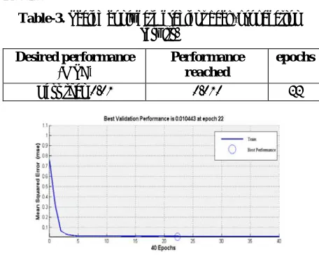
Table-3. Scaled conjugate gradient back-propagation results.

epochs

Less than 0.01 0.010 22

Figure-7. Performance graph of Scaled conjugate gradient back-propagation.

The figure here demonstrates the execution bend of the scaled conjugate calculation utilizing mse concerning the quantity of cycles over the preparation dataset. Amid the starting learning period of the preparation the execution was very much alike to that of angle plummet calculation creating a precarious incline down inside initial two cycles of the preparation yet beats it later on by coming to the best mse of 0.010 when contrasted with 0.014 from inclination drop inside 22 passes of the preparation dataset.

Momentum back-propagation algorithm

Not like in mini – batch machine learning, in Momentum method we utilize the adjustment in slope to redesign the speed and not the position of weight parts. In this system, we take the portion of the past weight overhauls and add that to the current one. The principle thought behind doing this is to enhance the productivity of the neural system by keeping the framework to join to a neighborhood least or to meet to a seat point.

Considering the fact that we have taken high momentum as a parameter which may help us accelerate the merging rate of the neural system, yet this may additionally cause the danger of overshooting the energy and making framework temperamental creating more capacity treks. Then again, in the event that we take force parameter little, it may happen that neural system adapts gradually. The tradeoff in the middle of high and low esteem must be remembered before picking the energy size for preparing.

Total number of hidden layer neurons used =639 Training function = traingdm

[image:4.612.75.299.116.277.2]

(5)

[image:5.612.73.300.132.307.2]

Results

Table-4. Momentum back-propagation results.

epochs

[image:5.612.317.544.292.443.2]

Less than 0.02 0.014 2

Figure-8. Performance graph of Momentum back-propagation.

Figure shows the performance curve of the momentum back-propagation using mse with respect to the number of iterations over the training dataset. The Steep drop in mse showing by the graph for the first two iterations is similar to that of gradient descent and SCG but it differs at a point that the best mse of 0.014, which is similar to that SCG and not too far from gradient descent, was achieved in first two epochs only. Although there was no any further/accountable decrease in network mse over the next few iterations continuously.

The figure demonstrates the execution bend of the Momentum back-proliferation utilizing mse concerning the quantity of emphases over the preparation dataset. The Precarious drop in mse indicating by the chart for the initial two cycles is like that of angle plunge and SCG yet it varies at a point that the best mse of 0.014, which is like that SCG and not very a long way from slope plummet, was attained to in initial two epochs, though there was no further/responsible decline in system mse, throughout the following couple of iterations persistently.

Adaptive learning rate back-propagation algorithm We have utilized multi-layer neural system, henceforth, we have to consider that there is a wide variety on what will be the suitable learning rate at every relating layer i.e. the particular inclination sizes at every layer are for the most part diverse. This circumstance spurs to utilize a worldwide learning rate in charge of every weight overhaul. With versatile learning system, the experimentation hunt down the best starting qualities for the parameters can be dodged. Ordinarily the adaption methodology has the capacity to rapidly receive from the beginning offered qualities to the proper ones. Likewise, the measure of weight that can be permitted to adjust relies on upon the state of the blunder surface at every specific circumstance. The estimations of the learning rate ought to be sufficiently expansive to permit a quick learning process additionally sufficiently little to ensure its adequacy. On the off chance that at some minute the quest

for the base is being done in the gorge, it is attractive to have a little learning rate, subsequent to generally the calculation will waver between both sides of the gorge.

Total number of hidden layer neurons =639 Training function = traingda

learningrate_increase = 1.04 .This helps determine the increase in the learning rate.

learningrate_decrease = 0.6 .This helps determine the decrease in the learning rate.

Results

Table-5. Adaptive learning rate back-propagation results.

epochs

Less than 0.02 0.014 2

Figure-9. Performance graph of Adaptive learning rate back-propagation.

The figure demonstrates the execution bend of the adaptive back – propagation utilizing mse regarding the quantity of cycles over the preparation dataset. Taking after the comparable example of mse (mean square error) bend as prior calculations the diminishment in mse demonstrated a lofty slant inside the initial couple of cycles over the dataset however it varies at a point that it had the capacity achieve the best mse of approx. 0.014 in 28 cycles. which by a long shot is the most elevated mse up till now obliging biggest number of iterations.

Momentum back-propagation with Adaptive learning

Rate back-propagation

This technique utilizes a combination of both momentum back-propagation strategy and the adaptive learning rate algorithm in order to train the neural network.

Total number of hidden layer neurons =639 Training function = traingda

(6)

Momentum = 0.9 . This helps determines the momentum constant used.

learning rate _increase = 1.04 .This helps determine the increase in the learning rate.

learning rate _decrease = 0.6 . This helps determine the decrease in the learning rate.

Results

Table-6. Momentum back-propagation with Adaptive learning rate back-propagation results.

epochs

Less than 0.01 0.014 3

Figure-10. Performance graph of Momentum propagation with Adaptive Learning Rate

back-propagation.

Here the figure demonstrates the performance graph of momentum back-propagation with adaptive learning algorithm using mse to the number of iterations on the training data input. This curve is quite similar to the adaptive learning rate algorithm technique and reaching a mse of 0.014. But this technique is much faster than the previous method where the number of total iterations required for this is 3 which is reduced from 28.

5.CONCLUSIONS

Beginning with performing distinctive analyses with all the different training algorithms to discover the best calculation with the most reduced conceivable mse on the preparation dataset, the outcomes from inclination drop and scaled conjugate angle plunge gave great mse when contrasted with other preparing calculations. The scaled conjugate slope drop delivered the slightest mse of 0.192 among all the preparation calculations, consequently kept preparing with more progressed systematic strategies utilizing these specific calculations setups as the premise for the analyses. In the arrangement of distinctive expository models, at first extremely encouraging results were accomplished with the assistance of the variety in the edge strategy which helped the score increment from 0.54 prior to 0.69 on the Innocentive leadership dashboard. In later phases of the examination, the procedure of retraining the effectively prepared systems for the imperative columns discovered exceptionally powerful in lessening the mse from 0.192 to 0.185.

The avoidance of commotion from the system further took mse to one of the best conceivable esteem so far accomplished.

At long last, as the last two methodologies looked exceptionally encouraging in expanding the system execution hence consolidate both the systems brought about a level 4 neural system which delivered the most reduced ever mse of 0.127 just, which was much closer to the craved mse of 0.1

6. FUTURE WORK

As the quantity of highlights in the application dataset increment, similar to on account of expansive scale applications, the layers size (neurons) of the fake neural system needs to be expanded to suit the expanded measurements of the information dataset. After certain point, the system size gets to be huge to the point that it gets to be very nearly infeasible to be executed effectively on account of the expanded unpredictability affected because of the exponential development of the between associations among the hubs (neurons) in the system. This marvel is by and large expressed as "the condemnation of dimensionality" in the field of machine learning. Along these lines, there is a need to turn out with a calculation to process extensive dataset productively keeping the neural system size significant little by upgrading the quantities of neurons and the interconnection between them.. The future work will be on streamlining the neural systems. There are a few paper distributed with diverse ways to deal with attain to this, yet the two most encouraging ones are hereditary calculations and particular configuration method.

REFERENCES

[1] Proceedings / International Work Conference on Artificial and Natural Neural Networks, IWANN '99. (1999). Berlin: Springer.

[2] Hassoun M. H. 1995. Fundamentals of artificial neural networks. Cambridge, Mass.: MIT Press.

[3] Bishop C. M. 1998. Neural networks and machine learning. Berlin: Springer.

[4] Wikipedia, Artificial neural network, 2007. [Online].[Accessed on 26th_{November 2014].} http://en.wikipedia.org/wiki/Artificial_neural_networ k.

[5] C. Stergiou& D. Siganos, Neural network, 1996. http://www.doc.ic.ac.uk/~nd/surprise_96/journal/vol4/ cs11/report.html.

(7)

[7] Gary Stein, Bing Chen, Annie S. Wu, and Kien A. Hua. 2005. Decision tree classifier for network intrusion detection with GA-based feature selection. In Proceedings of the 43rd_{annual Southeast regional} conference - Volume 2 (ACM-SE 43), Vol. 2.

[8] V. M. Rivas, J. J. Merelo, P. A. Castillo, M. G. Arenas and J. G. Castellano. 2004. Evolving RBF neural networks for time series forecasting with EvRBF, InformationSciences, 165, 207-220.

[9] Anderson, J. R., Michalski, R. S., Carbonell, J. G., and Mitchell, T. M. 1983. Machine learning: an artificial intelligence approach. Palo Alto, Calif.: Tioga Pub. Co.

[10]R. Nicole. “Title of paper with only first word capitalized,” J. Name Stand. Abbrev., inpress.

[11]Twinkle Bedi. 2014. “Green Cloud Computing using Artificial Neural Networks”, International Journal of Advanced Research in Computer Science and Software Vol. 4, No. 5, May.

[12]Azadeh S. F. Ghaderi and S. Sohrabkhani. 2007. Forecasting electrical consumption by integration of neural network, time series and ANOVA, Applied Mathematics and Computation, Vol 186, No. 2, pp. 1753-1761.