Study on Direct Numerical Simulation of Two dimensional Turbulence

2018 International Conference on Modeling, Simulation and Optimization (MSO 2018) ISBN: 978-1-60595-542-1

Study on Direct Numerical Simulation of Two-dimensional Turbulence

Fu-sheng QIU

_{, Yang LIU and Hong-juan ZHAO}

Shenyang Aerospace University, Shenyang, China *Corresponding author

Keywords: 2D turbulence, Direct numerical simulation, Vorticity-stream function method.

Abstract. Turbulence is one of the unsolved problems in fluid mechanics. The study of 3D

turbulence is very complex and difficult to achieve; while 2D turbulence is similar to 3D turbulence in many properties, and the related study is easier to carry out. Therefore, the study of 2D turbulence is significant to understand the characteristics of 3D turbulence. In this paper, the vorticity-stream function method is applied to the direct numerical simulation of 2D turbulence without any turbulence model. The third order Runge Kutta-Crank Nicholson method is used as the time integration method, and finite difference method of second order accuracy is for space discretization with central difference scheme and staggered grid. Turbulence conditions are used as boundary conditions and initial conditions. The vorticity distribution under different Reynolds number and different grid resolutions are obtained by numerical simulation. When the Reynolds number is low, the numerical discretization method with low order accuracy can resolve all vortex structures in space with higher grid resolution. But as the Reynolds number increases, the higher accuracy of the numerical discretization method is the best choice compared with the grid resolution enhancement.

Introduction

Direct numerical simulation (DNS) is an effective method to study turbulence. However, its complex numerical methods and the huge computational resources that required are daunting in 3D direct numerical simulation[1]. Although 2D turbulence is different from 3D turbulence in some respects, such as the inverse energy cascade characteristics[2]. 2D turbulence is similar to 3D turbulence in many properties, such as some statistical characteristics[3]. In addition, some 3D turbulence behave as 2D turbulence in some particular directions. Therefore, the study of the characteristics of 2D turbulent flow is of great significance for understanding that of the 3D turbulent flow.

It is difficult to simulate 2D turbulence under experimental conditions. Many scholars have made many attempts, for example, the 2D vortex formed by laminar flow through the cylinder shows 2D turbulence[4]. In contrast, numerical simulations seem to be easier to implement. In this paper, the vorticity-stream function method for 2D incompressible flow by direct numerical simulation is uesd with initial and boundary conditions of turbulence. The time integration is third order Runge Kutta-Crank Nicholson method, and the space discretization is second order finite difference method with central difference scheme and staggered grid. Finally, the vortices distribution at different time are obtained.

Governing Equations

It is difficult to solve the NS equations which describ 2D incompressible fluid flow because velocity and pressure are coupled. Here the vorticity-stream function method is used to eliminate the pressure term in the equation, which makes the solution easier. The dimensionless governing equations are 1-3.

2 2

2 2

1 Re

u v

t x y x y

      

 _  _  _  _

 

 

2 2

2 2

x y

  _

 _ _

  (2)

u v y x       

  (3)

Numerical Method

Time Discretization

Mixed third order Runge Kutta-Crank Nicholson method are taken for time integration. The product of vorticity and stream function is treated explicitly, and the second order derivative of vorticity is solved implicitly. This method avoids the strict restrictions on the time step if all items are explicitly processed and also avoids the problems that the large matrix is difficult to deal with if all of that are solved implicitly[5]. That is to ensure the accuracy of calculation and improve the computational efficiency at the same time. Then after the treatment, the equation 4 is changed to solve the first order ordinary differential equation of time derivative.

1 R e i i i d N L dt

 _{   (4)}

Although the Runge-Kutta method is one-step method, the third order accuracy method consists of three sub steps:





1

1 1 1

1 2 Re

n n n n

i i tNi tNi t Li Li

 _ _{ } _ _  _  _  _{ (5)}





2 2 2

1 2 Re n

i i tNi tNi t Li Li

 __{ }  _ _{ }  _ _  ₍₆₎





1 1

3 3 3

1 2 R e

n n

i i tNi tNi t Li Li

  __{ } _ _ _  _  _  (7)

Spatial Discretization

In this paper, the first order partial derivatives and the second order partial derivatives of the governing equations are discretized by the finite difference method with second order accuracy, and the central difference scheme is used. The finite difference method is simple in form and easy to program. The numerical simulation of 2D fluid flow requires small amount of computation at low Reynolds number. In this paper, the higher grid resolution is chosen to improve the numerical accuracy rather than the complex high order discretization method. The second order accuracy of first order partial derivative satisfies the calculation requirement, and the second order partial derivative has less influence on the calculation, so the second order accuracy is also used to discretize. In order to avoid the meaningless calculation results when the central difference scheme is applied to the calculation of incompressible fluid, due to the special treatment of boundary conditions or some other coincidences in the numerical solution, the staggered grid is adopted[6], and the linear interpolation is applied to the variable at the center.

 

 

, 1/ 2 , 1/ 2 2 ,

i j i j

i j

i j i j

 

 

1/ 2, , 1/ 2, 2

2 2

, 2

, 1/ 2 , , 1/ 2 2

2 2 , 2 1 4 2 1 4

i j i j i j

i j

i j i j i j

i j x x x y y y     _     _        _{ }     _{ }      (9)

Boundary Conditions and Initial Conditions

The application of real turbulent boundary conditions are very complicated. In this paper, the simplified turbulent boundary condition-the periodic condition-is applied in both two directions. That is, the values at the start and at the end are equal.

 

 

X i  X i n j X m j (10)

The variation of 2D turbulent flow depends on the initial conditions. The merging of vortices depends on the size and spatial distribution of the initial field[2]. The initial energy spectrum of the literature [7] is used. Firstly, the initial energy is obtained from the initial energy spectrum. Then the stream function values in wavenumber space are obtained with initial energy. Finally, the initial values of the stream function in physical space are obtained by Fourier transform.

 





0

, 0 exp /

E k Ck k k (11)











 



1, 2 1 2 1, 2 1, 2

E k k k k  k k  k k



 

  (12)

2 2 1 2

k k k (13)

 





1 2

1 2 2

1 /2 1

1 2 0 /2

, ,

N N

k i k j

k k N

i j k k e e 

   

 



 

Others

When the unsteady fluid flow is solved, it is necessary to ensure the convergence of the calculation in each time step, and the choice of time step depends on the CFL condition. The CFL condition can be understood as the time marching solution must be larger than the propagation velocity of the physical disturbance, and only in this way can all physical perturbations be captured. When the time marching method is used, the time step is the maximum time allowed by the CFL condition. In this paper, the theoretical value of CFL for RKCN method is 1.73.

The computational domain size is 22 with uniform grid.

1.73 1.73 min , max max x y t u v         

 (15)

Conclusion

The vorticity contours of different grid resolutions and different Reynolds numbers are calculated with the code which is written in Fortran. As shown in Figure 1 and Figure 2, the resolution is

obviously insufficient with the grid 128 128 , and the vortex structures that should be present do not

appear. After increasing the resolution to 256 256 , numerical oscillation still appears in the small

and thin vortices[8]. When the resolution continues to increase to 512 512 and 1024 1024 , the

But as the Reynolds numbers continue to increase, as shown in Figure 4, numerical oscillations still

occur in some areas even with the grid resolution of 512 512 . Numerical experiments show that

even if the grid resolution is increased to a high degree, the numerical oscillations will not disappear.

Figure 1. Vorticity contours of different grid resolutions at t10s,Re 5000 .

Figure 2. Vorticity contours of different grid resolutions at t10s,Re 5000 _.

That means, it is more effective to improve the accuracy of numerical discretization instead of grid accuracy. However, here the numerical oscillations in some regions where it’s not so important do not affect the study at higher Reynolds numbers.

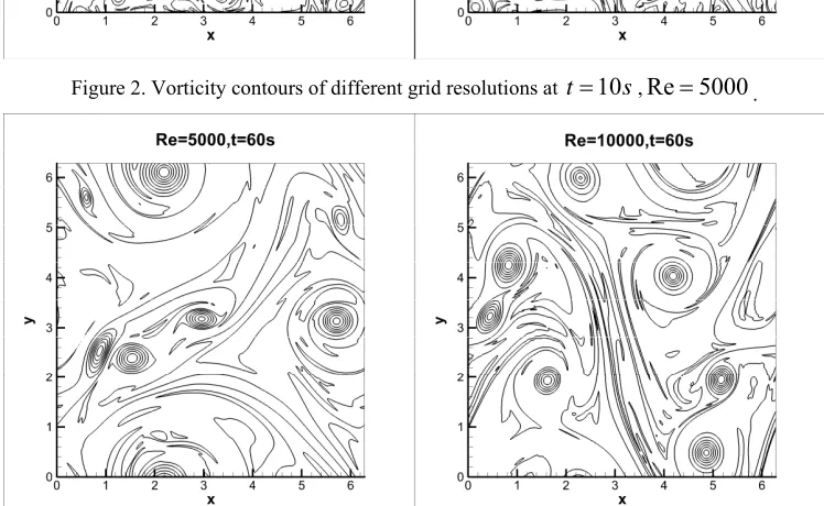
The 2D vortices will merge and eventually form a single dipole with the advance of time. As shown in Figure 3 and Figure 4, when the Reynolds number is high, the vortex merging rate decreases with time. In other words, the time of dipole emergence will get longer.

Figure 4. Vorticity contours of different Reynolds numbers at t60s,512 512 _.

Acknowledgement

This research was financially supported by the Foundation of Liaoning Educational Committee (L2013079).

References

[1] P. Moin, K. Mahesh, Direct Numerical Simulation: A Tool in Turbulence Research, J. Sci. Annual Review of Fluid Mechanics. 30 (1998) 539-578.

[2] P. Orlandi, Fluid Flow Phenomena: A Numerical Toolkit, Second ed., Springer Netherlands, Dordrecht, 2001.

[3] S.A. Orszag, G.S. Patterson, Numerical Simulation of Three-Dimensional Homogeneous Isotropic Turbulence, J. Sci. Physical Review Letters. 28 (1972) 76-79.

[4] D. Marteau, O. Cardoso, P. Tabeling, Equilibrium states of 2D turbulence: an experimental study, J. Sci. Physical Review E. 51 (1995) 5124-5127.

[5] Xi Jiang, Choi-Hong Lai, Numerical Techniques for Direct and Large-Eddy Simulations, first ed., CRC Press, Boca Raton, 2016.

[6] Y.Q. Zeng, Q.H. Liu, A staggered-grid finite-difference method with perfectly matched layers for poroelastic wave equations, J. Sci. Journal of the Acoustical Society of America, 109 (2001) 2571-80. [7] N.N. Mansour, AA Wray, Decay of isotropic turbulence at low Reynolds number, J. Sci. Physics of Fluids. 6 (1994) 808-814.