Panayotopoulos, Nikolaos, Lucas, Gary and Pradhan, Suman
Simulation of a four sensor probe using a rotating dual sensor probe
Original Citation
Panayotopoulos, Nikolaos, Lucas, Gary and Pradhan, Suman (2006) Simulation of a four sensor
probe using a rotating dual sensor probe. In: Proceedings of Computing and Engineering Annual
Researchers' Conference 2006: CEARC’06. University of Huddersfield, Huddersfield, pp. 16.
This version is available at http://eprints.hud.ac.uk/id/eprint/3807/
The University Repository is a digital collection of the research output of the
University, available on Open Access. Copyright and Moral Rights for the items
on this site are retained by the individual author and/or other copyright owners.
Users may access full items free of charge; copies of full text items generally
can be reproduced, displayed or performed and given to third parties in any
format or medium for personal research or study, educational or notforprofit
purposes without prior permission or charge, provided:
•
The authors, title and full bibliographic details is credited in any copy;
•
A hyperlink and/or URL is included for the original metadata page; and
•
The content is not changed in any way.
For more information, including our policy and submission procedure, please
contact the Repository Team at: [email protected].
Simulation of a four sensor probe using a rotating dual sensor
probe.
N. Panagiotopoulos, G. P. Lucas, P. Suman
ABSTRACT
In the current project a rotating dual sensor probe has been designed and fabricated. A set of measurements were performed using the rotating dual sensor. Analysis on the results occurred, and it showed that the rotating dual sensor with the supporting algorithm has an acceptable, reliable and repeatable performance for measurements in multiphase flows.
Keywords velocity components, conductivity probes, rotating probe, multiphase flows.
1 INTRODUCTION
.
In previous work of Lucas et al [1][2][3][4] the use of multi-sensor conductivity probes in bubbly multiphase flows is presented. It shows a method of fabricating two and four sensor probes, their electronic circuits and the resulting voltage waveform at their output. Also, it shows the signal processing scheme for extracting the bubble signature from the acquired signal, and the model for calculating flow properties of the dispersed phase in the pipe. Lucas et al compared the results from his measurements in different flow conditions with reference data and data from [5] and [6].
The multi-sensors that have been used by Lucas et al, were two sensor probe and four sensor probe. In literature [1][2][3][4], the description of their fabrication and the supporting electronic circuit can be found in detail. In the same literature, the signal processing and the calculation of the flow properties are described in detail too. As it can be seen, the two sensor probe is able to measure two flow properties of the disperse phase, which are the volume fraction and the axial velocity of the bubble. The four sensor probe is able to extract more information from the signals (due to the extra sensors), which is the vector velocity of the bubble.
Several measurements have been acquired using the two types of probes. The outcome of the analysis for the dual sensor probe showed that the whole system (probe, electronics, model, implementation of the algorithm in the computer, and visual presentation) performed very well with a small error. Detailed presentation of the performance of the dual sensor can be found in [3] and [4].
The four sensor probe showed results that exhibit some ambiguities and as a result from the previous description, a further investigation on the four sensor probe system was undertaken. So, a new test rig has been made, a new type of probe has been fabricated, and more data sets have been collected. Next, a detailed description of the rotating dual sensor probe is given.
2 LABORATORY
APPARATUS
.A bubble column was used in order to do the experiments. The bubble column has a bubble injector at the bottom, which is connected to a controllable air pump. The pump controls the amount of air that is inserted into the bubble column. A metal sheet over the air injector was positioned into the column. The metal sheet was drilled in many places having holes of a specific and identical diameter (6mm diameter). The pumped air from the injector was hitting the mesh and through the holes bubbles of almost 6mm diameter were created. Then the buoyancy force drives the bubbles straight to the top of the bubble column1.
Since it is desirable to measure bubble vector velocities, three parameters must be acquired. These are the polar angle or gamma (γ), the azimuthal angle or beta (β), and the velocity magnitude (v). It is important to mention that in the current work the azimuthal angle is defined as the angle between the y-axis and the projection of the vector on the x-y plane; also, the polar angle is defined as the angle between the z-axis and the vector. Positive azimuthal angles correspond to clockwise direction, and positive polar angles correspond to angles smaller than 900. This type of format is the
same with the one that was used in Mishra et al [2]. So, in order to be sure that the calculations of the model are correct, it is obligatory to acquire some reference data, in order to do the comparison and measure the error.
The reference data for the azimuthal β and polar γ angles can be acquired straight from the hinged probe holder and using an inclinometer. For the magnitude of the velocity vector (which is always vertical and parallel with the bubble column) a cross correlation meter was used. This is a pipe that fits into the bubble column and has two metal strips connected at its walls. The axial separation of these strips is 5cm. These metal pieces are connected with a set of cables. A two channel electronic set up has been built to support and drive the cross correlation meter. The electronic circuit was connected with a data acquisition. A software program (written in Visual Basic) was made to use the data acquisition unit. The acquired data were processed through another program (written in MatLab) to calculate the mean velocity of the bubbles.
As a result from the above, a bubble column system has been made for acquiring reference measurements and giving the advantage of a controllable and observable environment for the experiments. The figure below (figure 1) shows the system in a diagram.
Figure 1. Schematic of the bubble column and the instruments.
AIR PUMP Bubble
injector MESH
Cross Correlation electrodes
Driver for the Cross Correlation Meter DAC & PC with S/W
Bubbles
Cables
3
THE ROTATING PROBE
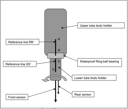
. [image:4.595.90.508.235.591.2]The rotating probe that was made is an original design and idea suggested by Lucas. It is a dual sensor but it has the ability to be rotated having the front sensor in the axis of rotation (and at the centre of the whole probe) and the rear sensor in any position that is desired. This type of probe can be used as a multi sensor probe (two sensor probe, four sensor probe, six sensor probe, 10 sensor probe, etc). In this paper it was used as a four sensor probe. The advantage of this type is that it has a smaller area of interface than the other probes, affecting the bubble’s motion less. Also, the design and fabrication of a dual sensor is simpler than a multisensor probe. The only disadvantage that this rotating dual sensor does have is that the flow condition must be in steady state during the measurements, while the other type of probes can be used in a non-steady state flow. But for the current work where the flow condition is in steady state, the specific disadvantage of the probe disappears. Figure 2 shows a drawing of the rotating dual sensor probe.
Figure 2. The rotating dual sensor probe.
Note that the upper part of the probe is clamped in the holder. As it was mentioned before, by rotating the lower tube of the probe in three distinct positions the result is to have a four sensor probe. For the current experiments, the rotation was clockwise and the angle step was 1200. So, the first position of the rear sensor was in 900 with respect to the x-axis (in a coordinate system that has as
origin the lead sensor), the second position of the rear sensor was 3300 (or -300), and the third position and the third position of the rear sensor was 2100. In other words, the first position of the rear sensor defines the y-axis of the, which passes from the lead and rear sensor. Also, based on figure 3, the first position of the rear sensor, makes the RR’ to be in line with SS’. In addition, the x-axis can be defined as any 900 degrees clockwise from the y-axis when viewed from the upper to lower tube of the probe. The (x,y,z) dimensions in mm of the virtual four sensor probe for each rear sensor with respect to the front sensor are: rear sensor 1 (0,0.7326,1.1765), rear sensor 2
(0.6344,-Waterproof Ring ball bearing
Lower tube body holder Upper tube body holder
Front sensor Rear sensor
Reference line RR’ R
R’
S
4
DUAL SENSOR PROBE’S ALGORITHM
After acquiring measurements from the rotating dual sensor probe, data processing has to be done. Next the algorithm that was used for processing the data is shown.
1. Stage 1: Calculate the numerator and denominator of
tan
( )
β
.2. Stage 2: Call N the result of numerator and D the result of denominator.
IF N>0 & D>0 THEN
=
−D
N
1tan
β
IF N>0 & D<0 THEN
−
⋅
=
−D
N
1tan
2
π
β
IF N<0 & D<0 THEN
+
=
−D
N
1tan
π
β
IF N<0 & D>0 THEN
−
=
−D
N
1tan
π
β
IF N=0 & D=0 THEN β=0
IF N=0 & D>0 THEN
2
π
β
=
IF N=0 & D<0 THEN
2
3
π
β
=
⋅
IF N>0 & D=0 THEN β=0 IF N<0 & D=0 THEN
β
=
π
3. Stage 3: Apply stages 1 and 2 to all 6 formulae of β.4. Stage 4: Find the β that gives positive γ angle. Those values are the correct ones.
5. Stage 5: Continue with the calculations of velocities (Azimuthial velocity, Radial Velocity, and Axial Velocity).
7) RESULTS OF THE NEW 4-SENSOR PROBE ALGORITHM.
The data that were used for testing the proposed algorithm were the same as the ones that are shown in table 1. Below, the results of data set 1 are presented when the rotating dual sensor probe and its algorithm are used. Each data set is a group of 5 flow conditions. For each flow condition the reference values of β, γ, and velocity are shown. As it was mentioned before, the reference β and γ are measured using an inclinometer and the probe holder, whilst the velocity magnitude is measured using a cross correlation instrument. Also, in the same table that presents the results of a flow condition, the β angle without considering the signs is shown for comparison reasons (this is the column that has “beta” as a label). Also the average time delays for each rear sensor are shown and they are labelled as “dt11”, “dt22”, and “dt33”.
Next, the data results using the new algorithm are presented.
SET 1
Reference DATA 1
beta: 0 dt11: 0.005207
gamma: 0 dt22: 0.005556
Vb_xcorr: 0.4026 dt33: 0.005675
beta gamma
Rotating probe 194.145 4.702547
Table 1
SET 1
Reference DATA 2
beta: 0 dt11: 0.006878
gamma: 24 dt22: 0.004833
Vb_xcorr: 0.4026 dt33: 0.004912
beta gamma
Rotating probe 358.0497 21.19236
SET 1
Reference DATA 3
beta: 180 dt11: 0.004164
gamma: 21 dt22: 0.005946
Vb_xcorr: 0.38845 dt33: 0.005887
beta gamma
Rotating probe 178.3495 19.39786
Table 3
SET 1
Reference DATA 4
beta: 90 dt11: 0.005428
gamma: 5 dt22: 0.005777
Vb_xcorr: 0.38845 dt33: 0.005637
beta gamma
Rotating probe 156.4698 3.325042
Table 4 SET 1
Reference DATA 5
beta: 270 dt11: 0.005631
gamma: 3 dt22: 0.005427
Vb_xcorr: 0.3743 dt33: 0.00576
beta gamma
Rotating probe 277.3747 3.174744
Table 5
SET 1 (measured velocities of the data)
Data Vaz Vrad Vax V
DATA 1 -0.00868 -0.03443 0.431614 0.433072
DATA 2 -0.00454 0.133465 0.344428 0.36941
DATA 3 0.004392 -0.15243 0.433075 0.459138
DATA 4 0.009724 -0.02233 0.419247 0.419954
DATA 5 -0.02299 0.002976 0.418032 0.418675
Table 6
8) COMMENTS ON THE RESULTS.
Visual inspection of the results, show that polar and azimuthal angles are very close to the reference values. It is important to mention again that for the flow conditions where the probe is vertical to the flow of bubbles there is no obligation that the azimuthal angle must be 00 degrees. It can take any value between 00 and 3590 degrees. Therefore, for this flow condition the value of β
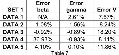
angle is not of great interest. The next two tables show the error percentage of polar, azimuthal, and velocity magnitude of the two data sets.
SET 1 Error beta gamma Error Error V
DATA 1 N/A 2.61% 7.57%
DATA 2 -1.08% -1.56% -8.24%
DATA 3 -0.92% -0.89% 18.20%
DATA 4 36.93% -0.93% 8.11%
[image:6.595.210.419.422.520.2]DATA 5 4.10% 0.10% 11.86%
Table 7
As it can be seen from the previous tables the polar angle is very close to the reference value and it is positive. This means that the flow is upwards and the algorithm could calculate the γ angle with an acceptable accuracy.
Figure 5. Oscillating plume [11].
It is also interesting how big the error of β for “DATA 4” flow condition becomes in both data sets. There is no currently any valid explanation regarding this case, therefore no comment can be said.
The polar angle is very close to the reference data. Looking at the tables, it is obvious that the error is small (less than 2%). This can be classified into the 95% confidence level in statistics.
9) Conclusions
Considering all the above, a new type of probe has been developed. Data have been acquired with the new probe and validated using the new algorithm. The results show a significant improvement for the calculation of azimuthal angle with a small errors comparing with the reference data. The comparison between the polar angles showed that a significant improvement has been achieved as well, with a small error (less than 2%). Also, a limitation has been proposed for the use of the specific algorithm. This limitation is that the knowledge of the direction of flow is essential and must be known.
REFERENCES
[1] G. P. Lucas and R. Mishra, “Measurement of bubble velocity components in a swirling gas-liquid pipe flow using a local four sensor conductance probe”, Measurements Science and Technology, vol. 15, pages 749-758, 2005.
[2] R. Mishra, G. P. Lucas, and H. Kieckhoefer, “A model for determining the velocity vectors of bubbles in a multiphase flow from seven time intervals measured using a four-sensor probe”, somewhere, sometime.
[3] N. Panayotopoulos, G. P. Lucas, and R. Mishra, “Calculation of volume fraction and mean bubble vector velocity using two and four sensor conductivity probes in vertical and inclined bubbly air-water flows”, School of Computing and Engineering Researchers’ Conference, Nov 2005.
[4] G. P. Lucas, R. Mishra, N. Panayotopoulos, “Power law approximation to gas volume fraction and velocity profiles in low void fraction vertical gas-liquid flows”, Flow Measurement and Instrumentation, vol. 15, pages 271-283, 2004.
[5] Van der Welle R 1985, “Void Fraction, bubble velocity and bubble size in two phase flow”, Int. J. Multiphase Flow, volume 11, pages 317-345.
[6] N. Zuber, J. A. Findlay, “Average volumetric concentration in two phase flow systems”, ASME J. Heat Transfer, vol. 87 (1965), pages 453-468.
[7] J. R. Grace and D. Harrison, “The influence of bubble shape on the rising velocities of large bubbles”, Chemical Eng. Science, vol. 22, pages 1337-1347, 1967.
[8] J. R. Crabtree and J. Bridgwater, “Bubble coalescence in viscous liquids”, Chemical Eng. Science, vol. 26, pages 839-851, 1970.
[9] Moshe Favelukis, Cam Hung Ly, “Unsteady mass transfer around spheroidal drops in potential flow”, Chemical Eng. Science, vol. 60, pages 7011-7021, 2005.
[10] Sergio Bordel, Rafael Mato, Santiago Villaverbe, “Modeling of the evolution with length of bubble size distributions in bubble column”, Chemical Eng. Science, vol. 61, pages 3663-3673, 2006.
![Figure 5. Oscillating plume [11].](https://thumb-us.123doks.com/thumbv2/123dok_us/382868.1038850/7.595.205.428.68.205/figure-oscillating-plume.webp)
