Three Papers on Asset Pricing
Petar Svilenov Sabtchevsky
Thesis submitted to the Department of Finance of the London
School of Economics and Political Science for the degree of
Doctor of Philosophy
Declaration
I certify that the thesis I have presented for examination for the PhD degree of the London School of Economics and Political Science is solely my own work other than where I have clearly indicated that it is the work of others (in which case the extent of any work carried out jointly by me and any other person is clearly identified in it).
The copyright of this thesis rests with the author. Quotation from it is permitted, provided that full acknowledgement is made. This thesis may not be reproduced without my prior written consent.
I warrant that this authorization does not, to the best of my belief, infringe the rights of any third party.
Statement of conjoint work
I confirm that Chapter 3 is jointly co-authored with Philippe Mueller, Andrea Vedolin, and Paul Whelan. I contributed 25% of the work for Chapter 3.
Acknowledgment
I would like to thank my academic supervisors Ian Martin and Georgy Chabakauri for their guidance and support. This thesis would not have been possible without the help I received from them. Both Ian and Georgy have been very patient, help-ful, inspirational, and valuable advisers throughout the course of my PhD studies. Whereas Ian introduced me to academic research during my first year on the PhD programme, Georgy’s lectures and research papers solidified my interest in contin-uous time general equilibrium models. I would also like to thank Peter Kondor. I immensely benefited from many discussions with him. He was always very ap-proachable and willing to discuss early stage research ideas. Additionally, I benefited from discussions with Thummim Cho, Victor DeMiguel, Christian Julliard, Martin Oehmke, Andrea Tamoni, and Dimitri Vayanos.
I am particularly indebted to my co-authors Andrea Vedolin, Philippe Mueller, and Paul Whelan. I would not be where I am now without their support. Andrea, Philippe, and Paul introduced me to the fascinating world of empirical research. I learned tremendously from numerous lively and eye-opening discussions with them. I am particularly grateful to Philippe and Paul for their continuous guidance and support.
Todorov, and Yue Yuan.
Abstract
This thesis consists of three papers on asset pricing.
In the first paper, I analyse the effects of volatility management (a trading strat-egy in which risky asset exposure is inversely proportional to the level of volatility) in a general equilibrium heterogeneous agent model. Two distinct types of agents popu-late the model economy, an unconstrained investor endowed with logarithmic utility over instantaneous consumption and a volatility-managed portfolio. My model goes a long way towards the rationalization of the behaviour of investment vehicles that follow investment management strategies that are isomorphic to the ones implied by the principles of volatility management. Whereas my theoretical approach offers a high degree of tractability, it is subject to some important caveats. Specifically, the model implies unrealistically high leverage for the unconstrained investor.
In the second paper, I propose a general equilibrium intermediary asset pricing model featuring a heterogeneous intermediary sector. Two distinct types of interme-diaries populate the financial intermediary sector: equity-constrained intermeinterme-diaries and shadow financial intermediaries. The main theoretical contribution of this pa-per is threefold. First, I show that over the region of the state space where the intermediation constraint binds, the risk premium on the intermediated risky asset is decreasing in the degree of intermediary sector heterogeneity. Second, intermedi-ary sector heterogeneity allows for rich leverage dynamics within the intermediintermedi-ary sector and at the level of the aggregate intermediary sector. Third, the constrained region shrinks relative to the benchmark model in which the intermediary sector is homogeneous.
1 Volatility-Managed Portfolios in General Equilibrium 13
1.1 Introduction . . . 14
1.2 Model . . . 21
1.2.1 Assets . . . 22
1.2.2 Volatility-Managed Portfolios . . . 23
1.2.3 Unconstrained Investors . . . 28
1.2.4 Equilibrium Conditions . . . 30
1.3 Characterization of Equilibrium . . . 31
1.3.1 Main Results . . . 31
1.4 Analysis of Equilibrium (Main Case, ρ > ρv) . . . 37
1.4.1 Comparative Statics . . . 41
1.5 Analysis of Equilibrium forρ < ρv . . . 42
1.6 Broader Perspective and Discussion . . . 46
1.6.1 Implications of Homogeneous Agent General Equilibrium Mod-els . . . 46
1.6.2 Relation to Moreira and Muir (2017) . . . 47
1.6.3 Relation to Martin (2017) . . . 48
1.7 Conclusion . . . 49
1.8 Mathematical Appendix . . . 50
1.8.1 Portfolio Choice of the Risk-neutral Investor . . . 50
1.8.2 Portfolio Choice of the Unconstrained Investor . . . 52
1.8.4 Proof of Proposition 1 (Model-Implied Total Return Process
Volatility) . . . 53
1.8.5 Proof of Proposition 2 (Properties of Total Return Process Volatility) . . . 55
1.8.6 Proof of Proposition 3 (Risk Premium) . . . 56
1.8.7 Proof of Proposition 4 (Quadratic Co-variation) . . . 59
1.8.8 Proof of Proposition 5 (Properties of Quadratic Co-variation) 61 1.8.9 Proof of Proposition 6 (Portfolio Sensitivities) . . . 63
1.8.10 Proof of Proposition 7 (Equilibrium, Baseline Model) . . . 63
1.8.11 Derivation of the Equilibrium Risk-free Interest Rate . . . 65
2 Intermediary Asset Pricing with Heterogeneous Financial Interme-diaries 78 2.1 Introduction . . . 79
2.2 Model . . . 86
2.2.1 Assets . . . 88
2.2.2 Equity-Constrained Financial Intermediary . . . 89
2.2.3 Households . . . 92
2.2.4 Shadow Financial Intermediary . . . 94
2.2.5 Equilibrium Conditions . . . 95
2.2.6 Stochastic Discount Factor (SDF) . . . 97
2.3 Model Solution . . . 97
2.3.1 Separating Boundary . . . 98
2.3.2 Risk Premium . . . 100
2.3.3 Characterization of Equilibrium . . . 101
2.3.4 Price-Dividend Ratio . . . 106
2.3.5 Model-Implied Leverage Dynamics . . . 107
2.3.6 Discussion of Results and Economic Intuition . . . 109
2.4 Conclusion . . . 114
2.5.1 Euler Equation of the Equity-Constrained Financial
Interme-diary . . . 115
2.5.2 Portfolio Choice . . . 115
2.5.3 Price-Dividend Ratio . . . 119
2.5.4 Volatility of the Total Return Process . . . 120
2.5.5 Leverage Dynamics . . . 122
2.5.6 Proof of Proposition 8 (Separating Boundary) . . . 123
2.5.7 Proof of Proposition 9 (Equilibrium, Both Constraints Bind) . 123 2.5.8 Proof of Proposition 10 (Equilibrium, Only the Intermediation Constraint Binds) . . . 124
2.5.9 Proof of Proposition 11 (Equilibrium, Only the Leverage Con-straint Binds) . . . 124
2.5.10 Proof of Proposition 12 (Equilibrium, Neither Constraint Binds)124 2.5.11 Proof of Proposition 13 (Equilibrium Quantities, Properties) . 124 2.5.12 Separating Boundary (Leverage Constraint) . . . 125
2.6 Appendix (Figures) . . . 128
2.7 Appendix (Tables) . . . 136
3 Variance Risk Premia on Stocks and Bonds 138 3.1 Introduction . . . 139
3.2 Estimation of Expected Variance . . . 145
3.2.1 Data . . . 146
3.2.2 Variance Trading and Variance Risk Premia . . . 148
3.2.3 Physical Variance . . . 149
3.2.4 Implied Variance . . . 152
3.3 Descriptive Analysis . . . 153
3.3.1 Basic Properties. . . 154
3.3.2 Time-Series Evidence . . . 154
3.3.3 Co-movement . . . 157
3.4.1 Univariate Regressions . . . 159
3.4.2 Multivariate Regressions . . . 161
3.4.3 Controls . . . 162
3.5 Real Nominal Risks . . . 164
3.6 Conclusion . . . 169
3.7 Appendix (Figures) . . . 171
2.1 Intermediary Asset Pricing with Heterogeneous Financial
Intermedi-aries, Parameter Values . . . 137
3.1 Summary Statistics (Futures Excess Returns) . . . 179
3.2 Summary Statistics (Implied Volatilities and Variance Risk Premia) . 180
3.3 Return Predictability Regressions (Univariate) . . . 181
3.4 Return Predictability Regressions (Multivariate) . . . 182
3.5 Equity Return Predictability Regressions (Controls) . . . 183
3.6 10y Treasury Futures Return Predictability Regressions (Controls) . . 184
3.7 Real versus Nominal Risks (Full Sample) . . . 185
3.8 Real versus Nominal Risks (Post 2000 Sample TIPS regressions) . . . 186
3.9 Real versus Nominal Risks (Post 2000 Sample Nominal regressions) . 187
1.1 Model Solution, Case ρ > ρv (zoomed-in version) . . . 67
1.2 Model Solution, Case ρ > ρv . . . 68
1.3 Model Solution, Case ρ < ρv (zoomed-in version) . . . 69
1.4 Model Solution, Case ρ < ρv . . . 70
1.5 Quadratic Co-variation and Sharpe Ratios, Case ρ > ρv . . . 71
1.6 Quadratic Co-variation and Sharpe Ratios, Case ρ < ρv . . . 72
1.7 Price-Dividend Ratio . . . 73
1.8 Relation to Martin (2017) (zoomed-in version) . . . 74
1.9 Relation to Martin (2017) . . . 75
1.10 Comparative Statics (zoomed-in version) . . . 76
1.11 Comparative Statics . . . 77
2.1 Model Diagram . . . 129
2.2 Separating Boundary . . . 130
2.3 Risk Premium . . . 131
2.4 Risk Premium (zoomed-in version) . . . 132
2.5 Total Return Process Volatility . . . 133
2.6 Total Return Process Volatility (zoomed-in version) . . . 134
2.7 Portfolio Policy Functions . . . 135
3.1 Expected Physical and Risk Neutral Volatility . . . 171
3.2 Equity and Treasury Variance Risk Premia . . . 172
3.3 Standardized Variance Risk Premia . . . 173
3.4 Conditional Correlations between Equity and Treasury Returns . . . 174
3.5 Conditional Correlations between Treasury and Equity Variance Risk
Premia . . . 175
3.6 Variance Risk Premia around LTCM and Tamper Tantrum . . . 176
3.7 Futures Excess Returns Long Horizon Predictability (R2) . . . 177
Volatility-Managed Portfolios in
General Equilibrium
1.1.
Introduction
The volatility-managed trading strategy requires that the size of the risky asset position is inversely proportional to the level of volatility. Traders that follow volatility-managed trading strategies decrease their risky asset exposure in high-volatility states and increase risky asset exposure in low-high-volatility states. Given that volatility tends to be high in adverse states of the world, investors following a volatility-managed trading strategy would decrease their exposure at times of severe market dislocations and re-enter the market at times when market conditions are more favorable.
Volatility management constitutes a profitable trading strategy so long as asset volatility and the risk premium do not move in lockstep; that is, an increase in volatility is not immediately followed by a corresponding increase in the risk pre-mium. If that is the case, an increase in asset volatility leads to a drop in the Sharpe ratio that renders the risky asset less attractive1 and justifies portfolio rebalancing towards the risk-free asset.
The sign of the correlation between expected returns and conditional variance is the subject of a heated debate. Conventional wisdom suggests that it is prudent to increase risk taking, or at the very least keep it constant, during economic downturns when volatility tends to be high. Investors failing to follow this advice are warned that they risk missing out on a once-in-a-generation buying opportunity at their own peril. This type of advice is put forward not only by leading practitioners, such as Warren Buffet, CEO of Berkshire Hathaway, but also by leading financial economists such as John Cochrane of the University of Chicago. Cochrane goes so far as to argue that
If you’re less leveraged, less affected by recessions, and have a longer horizon than the average, it makes sense to buy. If you’re more leveraged, more affected by recession or have a shorter horizon, it might be the time
to sell, even though you might be cashing out at the bottom. If you’re about the same as everyone else, do nothing and relax. If you’re wrong, at least you will have excellent company.
In a widely cited paper, Fama and French (1989) show, in line with the con-ventional view, that expected returns are high during recessions. On the theoret-ical front, the trading recommendation is broadly the same. Prominent off-the-shelf, single-agent equilibrium models, Bansal and Yaron (2004) andCampbell and Cochrane (1999), among others, imply a positive sign for the correlation between conditional volatility and expected returns. Clearly, the conventional view advocates for a portfolio trading strategy that is in many respects the opposite of a portfolio strategy devised in the spirit of volatility management.
In a recent paper, Moreira and Muir (2017) challenge this conventional view. They empirically show that conditional variance is only weakly related to future expected returns and the increase in expected returns is nowhere big enough to compensate investors for the increase in volatility. They also show that volatility-managed portfolios, scaled by the inverse of previous month’s realized variance, earn large risk-adjusted alphas across a wide range of asset pricing factors, hinting at the possibility that the expected return conditional volatility trade-off weakens in high-volatility states of the world. In a companion paper,Moreira and Muir (2016) show that volatility timing is optimal for a very wide range of investors, both short-term and long-term investors, and volatility timing leads to substantial utility gains on the order of 35% of lifetime utility. These results are, however, subject to some impor-tant caveats. First, the results are sensitive to the volatility measurement horizon. The authors use a relatively short horizon of one month. Second, the authors use
high.
The recommendation for volatility timing implied by Moreira and Muir (2016) andMoreira and Muir(2017) poses a formidable puzzle, because it is not only at odds with the conventional view described above but it is also somewhat problematic from the perspective of standard general equilibrium asset pricing models. This is because standard equilibrium models imply countercyclical risk aversion, countercyclical risk premia, and countercyclical volatility.
The main objective of this chapter is to rationalize the volatility-managed trad-ing strategy and, by dotrad-ing so, reconcile the puzzle posed byMoreira and Muir(2016) and Moreira and Muir (2017). To this end, I develop a heterogeneous agent model cast in continuous time and study the model-implied pure exchange economy with heterogeneous agents. Unconstrained agents endowed with logarithmic utility over instantaneous consumption and investors following a volatility-managed investment strategy are the two different types of agents that populate the model economy. While the unconstrained investors admit the interpretation of sophisticated finan-cial market participants, the volatility timers map well to fund managers with an investment mandate to time and manage volatility.
It is instructive to note that the modeling approach I take is very different from the modeling approach inMoreira and Muir(2017). InMoreira and Muir(2017), the authors take a partial equilibrium perspective, and I propose a general equilibrium model featuring heterogeneous agents. Whereas in the partial equilibrium setups of
The main theoretical contribution of this chapter is threefold. First, my model goes a long way towards the rationalization of the volatility-managed trading strat-egy (i.e., the risky asset position inversely proportional to the level of volatility). Namely, I show that the volatility-managed trading strategy constitutes a profitable trading strategy in my model economy, so long as some mild parameter restrictions are satisfied. This is because, in my model economy, the model-implied volatility and the risk premium are negatively correlated over the entire state space, and the risk-return trade-off, as measured by the Sharpe ratio, deteriorates in high-volatility states. Thus, an investor leaving the market in high-volatility states does not sacri-fice the opportunity of earning a high risk premium. On the other hand, an investor that loads on the market in low-volatility states earns very high expected returns in risk-adjusted terms.
Second, I argue that the parametric restriction that delivers the above results is likely to hold in reality. For volatility timing to be profitable in my model economy, the fund management fee charged by volatility-managed portfolios should be lower than the subjective discount factor of the unconstrained investors. This is likely to hold in reality for the following reason. Volatility-managed portfolios effectively follow a passive investment strategy that is easy and cheap to implement. Fund managers following passive investment strategies are only able to charge very low fund management fees, and their fees are usually on the order of a few dozen basis points (i.e., very close to zero). Given that the subjective discount factor (i.e., the consumption-to-wealth ratio) of the unconstrained investor is a positive number, the above parameter restriction is likely to hold.
models that imply countercyclical risk premia.
Additionally, volatility timers exert positive externalities on the unconstrained agents, the centerpiece of my model. Being insensitive to the risk-return trade-off, volatility timers only use conditional volatility as an input to their portfolio construction process. This trading behavior, on the part of the volatility timers, creates distortions that the unconstrained investors can exploit to their advantage. Finally, the model allows me to study how the volatility timers affect equilibrium quantities of interest for different relative sizes of the asset management industry explicitly engaged in volatility timing.
The theoretical results that I report are subject to some caveats. That is to say, the model-implied leverage of the unconstrained investor is counterfactually high over the entire state space.
Related Literature
This paper closely relates to three different strands of the literature. First, it is re-lated to the literature on portfolio management and volatility management. Second, it is related to the literature studying the effects of portfolio insurance in general equilibrium. Third and finally, it also relates to the literature on equilibrium models with heterogeneous agents.
In a series of recent papers, Moreira and Muir (2017) and Moreira and Muir
(2016) empirically show that trading strategies devised in the spirit of volatility management deliver high Sharpe ratios and high risk-adjusted alphas. They further show that conditional volatility and expected returns are only weakly correlated, and the correlation weakens in high-volatility states. In a follow-up paper, Moreira and Muir(2016), the authors show that volatility management is optimal for a wide range of investors, both short term and long term.
Conceptually, the volatility-managed portfolios are the modern-day reincarna-tion of portfolio insurance, a dynamic hedging strategy developed by Hayne Leland, John O’Brien, and Mark Rubinstein in the 1970s. Portfolio insurance gained popu-larity in the 1980s as a way to protect investment portfolios against market down-turns. Two prominent papers, Grossman and Zhou (1996) and Basak (1995), use martingale techniques to study portfolio insurance in a general equilibrium context. In their classic paper, Grossman and Zhou(1996) show that portfolio insurance in-creases price volatility, induces mean reversion in asset returns, and inin-creases the Sharpe ratio and volatility in bad states of the world. There are similarities between these two papers on portfolio insurance and my paper. In the papers on portfolio insurance, portfolio insurers exit the market when the market drops. In my paper, volatility-managed portfolios exit the market when volatility rises. To the extent that market declines and volatility increases are perfectly correlated, portfolio in-surance is similar to volatility timing.
downward-sloping demand curve. Rytchkov (2014) studies the equilibrium effects of dynamic margin constraints in a dynamic heterogeneous agent economy cast in continuous time. In his paper,Rytchkov (2014) shows that a dynamic margin constraint, where the tightness of the constraint is proportional to the volatility of the total return process, results in a portfolio choice that is consistent with the principles of volatil-ity management. The main difference between my paper and that of Rytchkov
(2014) is that the volatility limit in my model binds over the entire state space. More importantly, the model proposed in Rytchkov (2014) is much less tractable compared to my model. Whereas Rytchkov (2014) resorts to numerical solution techniques, I derive all equilibrium quantities of interest in closed form. My paper is also related to Basak and Pavlova (2013), who study the effects of institutional investors on asset prices in equilibrium. Retail and institutional investors are the two types of agents that populate the model economy inBasak and Pavlova (2013). Whereas retail investors are endowed with logarithmic utility over terminal wealth, the marginal utility of institutional investors is increasing in the level of the stock market index. Interestingly, the optimal portfolio policy function of the institutional investors in Basak and Pavlova(2013) features a component that very much resem-bles a volatility-managed portfolio. This component is, however, small in magnitude, a fact that renders the model proposed byBasak and Pavlova(2013) impractical for the study of volatility management in equilibrium.
perspective and discuss how they relate to some prominent papers on volatility management. Section 1.7 concludes. Finally, in the mathematical Appendix, I provide detailed derivations of all results from the main body of the chapter.
1.2.
Model
I consider an infinite-horizon heterogeneous agent pure exchange economy cast in continuous time. The economy is populated by two distinct types of agents, dy-namic volatility timers and unconstrained investors optimizing over instantaneous consumption.
The dynamic volatility timers follow a volatility-managed trading strategy. Namely, they increase their risky asset exposure in low-volatility states and decrease their risky asset exposure in high-volatility states. As I show below, volatility timing constitutes an optimal portfolio strategy from the vantage point of a risk-neutral in-vestor subject to a risk limit (volatility budget) that is reminiscent of a value-at-risk (VaR) constraint. Given that they are risk neutral, the volatility timers populating the model economy admit the interpretation of trading desks at a large financial intermediary operating under a value-at-risk (VaR) constraint. It is also possible to map the volatility timers of the model to investment management funds with an in-vestment mandate stipulating the maintenance of a certain volatility level (volatility budgeting) or even outright volatility timing. Risk parity funds, for example, Bridge-water All Weather, AQR Risk Parity Fund, and Invesco Balanced Risk Allocation Fund, are prominent examples of the former, and volatility-managed portfolios, for example, Goldman Sachs Global Markets Navigator Fund, and AllianceBernstein Dynamic Asset Allocation Portfolio, are examples of the latter.
finan-cial market participants with relatively long investment horizons or to asset/wealth managers with long-term discretionary investment mandates. It is one of the main objectives of this chapter to study how the volatility-managed portfolios affect un-constrained investors.
I solve the model in terms of the wealth share of the unconstrained investor, which is the state variable of the model. My model is unusually tractable for a model that belongs to the class of heterogeneous agent models. That all equilibrium quantities of interest are available in closed form allows me to present the theoretical results of the chapter in a very accessible and straightforward manner.
1.2.1. Assets
Here, I describe the financial assets on offer to the agents of the model. There is a risk-free asset with an instantaneous rate of return equal to r(·). The risk-free asset is in zero-net supply, and I solve for the endogenous risk-free interest rate. Below, I show thatr(·) is a function of the state variable of the model, which is the wealth share of the unconstrained investor. There is also a single risky asset that is a claim to the dividend stream, {Dt}. The risky asset admits the interpretation of a dividend-paying common stock. Following convention in the literature, I assume that the risky asset is in a positive net supply of one unit. The stochastic differential equation
dDt
Dt
=µDdt+σDdBt (1.1)
governs the dividend growth process, {Dt}. The drift, µD ∈ R++, and the
diffu-sion, σD ∈ R++, coefficients are positive and exogenous constants. The diffusion
coefficient, σD, measures the amount of fundamental risk in the economy. Clearly, dividend growth is i.i.d. as implied by the above stochastic differential equation.
{Bt} is a standard one-dimensional Wiener process.2
2The Wiener process,{B
t}, is defined on the filtered probability space (Ω,F,F,P). I denote
Let St be the time-t price of the risky asset. Then, the total return process, {Rt}, follows the drift-diffusion process
dRt =
Dtdt+dSt
St
,
where Dt/Stdt admits the interpretation of income gain (dividend-income) per unit of time-dt, anddSt/Stis capital gain. In the following sections, I derive an expression for the endogenous price-dividend ratio, St/Dt, of the risky asset and show that it is a function of the state variable of the model.
In the model, the Brownian shocks driving the dividend growth process are the only source of randomness. Consequently, as I am going to show in the sequel, the dividend process, {Dt}, and the risky asset price process, {St}, are driven by the same Brownian motion. I conjecture, and will later on verify the conjecture, that the total return process follows a drift-diffusion,
dRt=µR(·)dt+σR(·)dBt,
where µR(·) and σR(·) are the equilibrium drift and diffusion coefficients, respec-tively. I allow all agents of the model to trade both the risk-free and the risky assets.
1.2.2. Volatility-Managed Portfolios
Here, I introduce volatility-managed portfolios that are isomorphic to the ones im-plied by the principles of volatility timing.
One possible way to generate a managed volatility portfolio is to solve a dynamic constrained portfolio optimization problem from the vantage point of a short-horizon myopic risk-neutral investor subject to a risk limit (volatility budget). I denote the time-t wealth of the risk-neutral investor by ˜Wt, her instantaneous consumption by satisfies theusual conditions; that is, the filtration is complete and right-continuous. A process in this chapter is by definition a stochastic process that is progressively measurable with respect to
˜
Ct, and I assume that the agent consumes a constant fraction, ρv, of her wealth, ˜
Ct=ρvW˜t.
It is sensible to assume that the instantaneous consumption of the fund manager equals a constant fraction of wealth under management, where the latter admits the interpretation of a fund-management fee levied on assets under management (ex-ogenous compensation contract). Let ˜θtbe the portfolio policy of the fund manager expressed as a fraction of time-t wealth. Then, the stochastic differential equation
dW˜t =(rtW˜t−C˜t)dt+ ˜θtW˜t(dRt−rtdt)
fully characterizes the intertemporal wealth evolution of the volatility timer. The first term on right-hand side, rtW˜tdt, is the instantaneous risk-free return of the investor, and ˜θtW˜t is the dollar size of her risky asset position. Using the fact that the consumption rate is constant, the stochastic differential equation simplifies to
dW˜t=(rt−ρv) ˜Wtdt+ (µR(·)−rt)˜θtW˜tdt+σR(·)˜θtW˜tdBt,
whereµR(·) andσR(·) are the conjectured drift and diffusion coefficients of the total return process, {Rt}. Clearly, the portfolio policy, ˜θt, is the only choice variable of the volatility timer. The myopic volatility timer maximizes next-period consump-tion, ˜Ct+dt, subject to a volatility budget, and to a dynamic budget constraint,
max
{θ˜t} Et
˜
Ct+dt
,
s.t. θ˜t≥0,
β
s
Vart(dW˜t)
dt ≤
˜
Wt,
where the risk limit (volatility budget) is the second constraint, and the dynamic budget constraint is the third one. The long-only restriction, ˜θt ≥ 0, squares well with the stylized fact that volatility-managed portfolios tend to be structured as long-only investment vehicles.
The risk limit (volatility budget) very much resembles a value-at-risk (VaR) constraint. Namely, β-times the risk of the portfolio, as measured by the forward-looking standard deviation of portfolio returns, admits the interpretation of value-at-risk. Parameter β ∈R++ is an exogenous parameter controlling the tightness of
the constraint. Clearly, the tightness of the constraint is increasing in parameter
β. The exogeneity of this parameter is without loss of generality. It is usually imposed on financial intermediaries by regulatory bodies. In the context of asset management, the investment mandate of the investment vehicle establishes what values β should take. The identity
Vart(dW˜t) = dhW ,˜ W˜it
allows me to calculate the instantaneous variance of wealth from the quadratic variation of {Wt}. Following convention, I use the notation h·,·i to denote the square-bracket process (quadratic variation). Given the facts that ˜Wt depends on past portfolio choices, ˜Ct = ρvW˜t, and ρv is a constant, ˜Ct is pre-determined as of time-t. Consequently,
argmax(Et( ˜Ct+dt)) = argmax(Et(dC˜t)) = argmax(Et(dW˜t)).
Therefore, it is enough for an agent with the objective of maximizing next-period consumption to maximize the increase in the value of assets under management,
Danielsson, Shin, and Zigrand (2010),
max
{θ˜t} Et
dW˜t
dt
!
,
s.t. θ˜t≥0,
β
s
Vart(dW˜t)
dt ≤W˜t,
dW˜t = (rtW˜t−C˜t)dt+ ˜θtW˜t(dRt−rtdt).
The constraints are the same as above. The only difference between the two opti-mization problems is in the objective function. Here, I maximize expected wealth growth as opposed to next-period consumption.
Absent the risk limit (volatility budget) and under the assumption that the expected total return on the risky asset is positive, the risk-neutral investor sets ˜
θt = ∞ and, by doing so, prices the unconstrained investor out of the market. In the presence of a risk limit (volatility budget), however, this strategy is no longer feasible, and the agent behaves as if she is risk averse. Namely, the volatility timer sets the size of her risky asset position in such a way so as not to violate her volatility budget. Additionally, the tightness of the constraint is inversely proportional to the endogenous wealth level, ˜Wt, of the agent. Negative shocks to wealth (assets under management), ˜Wt, erode the capital position of the agent and inhibit her ability to take large risky asset positions.
Expected wealth growth and its conditional variance immediately follow from the stochastic differential equation governing the intertemporal wealth evolution of the wealth of the volatility timer,
Et(dW˜t) =(rt−ρv) ˜Wtdt+ (µR(·)−rt)˜θtW˜tdt, Vart(dW˜t) =(σR(·)˜θtW˜t)2dt.
over the entire state space and the risky asset earns a positive risk premium. This fact immediately implies that the constrained portfolio optimization problem of the risk-neutral investor admits the solution:
˜
θt= 1
β
1
σR(·)
.
This is because ˜θtonly takes non-negative values, and the constraint associated with the risk limit(volatility budget),
β
s
Vart(dW˜t)
dt ≤
˜
Wt,
binds with equality. It is convenient to define ¯σ = 1/β. The newly defined param-eter, ¯σ, admits the interpretation of a risk limit. Clearly, the tightness of the risk limit is decreasing in ¯σ. For high values of ¯σ, the agent can take high leverage. Using the newly defined parameter, I can rewrite ˜θt,
˜
θt= ¯
σ σR(·)
.
I assume that the principal of the constrained risk-neutral investor sets the exoge-nous risk limit in such a way so as to satisfy the inequality ¯σ < σD. This parameter restriction inhibits the ability of the volatility timer to maintain a high leverage ratio. It is, however, without loss of generality and broadly in line with prevailing practice in the fund management industry. Funds with investment mandates to time volatility tend to maintain low leverage ratios, usually below one.
It is important to keep in mind that ˜θtexpresses the portfolio choice of the agent as a fraction of total wealth. Consequently, the dollar size of the risky asset position of the agent is
¯
σ σR(·)
˜
The portfolio choice of the risk-neutral agent facing a risk limit (volatility budget) is a valid volatility-managed portfolio. This is because the size of the risky asset position is inversely proportional to the level of volatility of the risky asset. More importantly, the expected return on the risky asset, µR(·), appears nowhere in this expression. This is the defining characteristic of the volatility-managed portfolio. At the same time, it is also the main point of difference between a myopic mean-variance portfolio and a volatility-managed portfolio. Additionally, the size of the risky asset position is inversely proportional to the tightness of the constraint. Finally, the volatility-managed portfolio depends on the wealth level, ˜Wt, of the agent. In this respect, the volatility-managed portfolio resembles the optimal portfolio of an investor endowed with logarithmic utility, or the portfolio of a constant relative risk aversion (CRRA) investor, if we were to abstract from the hedging demand term. The agent is nominally risk neutral, but behaves as if risk averse, because of the constraint. The effective risk aversion is inversely proportional to the wealth level.
1.2.3. Unconstrained Investors
Here, I introduce the group of unconstrained logarithmic utility investors. They admit the interpretation of sophisticated financial players or asset managers with flexible (discretionary) long-term investment mandates. The unconstrained investors are the centerpiece of my model. One of my main objectives is to study how the unconstrained and fully rational investors are affected by the volatility-managed portfolios that they co-exist with in the model economy. In equilibrium, prices have to adjust so that the unconstrained investors are happy to take the other side of the trade. The unconstrained investors are identical and form a continuum of measure one. The representative unconstrained investor solves the intertemporal consumption-portfolio choice problem,
max
{Ct,θt} E
Z ∞
0
e−ρtu(Ct)dt
subject to the dynamic constraint
dWt =rtWtdt−Ctdt+θtWt(dRt−rtdt), (1.2) where the stochastic differential equation governs the intertemporal wealth evolution (between time t and time t+dt) of the representative unconstrained agent and
u(Ct) = ln(Ct), Ct >0.
The first term on the right-hand side of (1.2) is the instantaneous return on the investment in the risk-free asset. The second and the third terms are instantaneous consumption and risky asset excess return, respectively. Additionally, ρ ∈ R++ is
the subjective discount factor of the agent, Wtis wealth, and dRt−rtdt is the total
excess return on the risky asset. Finally, θt is the portfolio choice expressed as a fraction of total wealth, Wt, and θtWt is the dollar size of the risky asset position.
In the main version of the model, I assume that ρ > ρv. Below, I am going to argue that this inequality is likely to hold in reality. While ρ is the consumption-to-wealth ratio of the unconstrained investor, ρv admits the interpretation of the fund management fee that the volatility-managed portfolios charge. Given that in its simplicity the volatility-managed strategy resembles a passive trading strategy, it is not unrealistic to assume that volatility-managed portfolios are only able to charge very low fund management fees on the order of a few dozen basis points. So long as volatility management portfolios charge a low fund management fee, ρv will be positive but will be very close to zero, and ρ > ρv is likely to hold.
the representation
θt= 1
xt − σ¯
σR(·) 1−xt
xt
,
where
xt=.
Wt
St
is the state variable of the model, which is the wealth share of the unconstrained investor. Clearly, in a pure exchange economy xt∈[0,1]. In the following sections, I explicitly solve for σR(·) and show that it is a function of the state variable, xt.
1.2.4. Equilibrium Conditions
In this subsection, I formally define the equilibrium concept used to solve the model. After enlisting all equilibrium conditions, I outline the model solution strategy that I follow in the following sections.
Definition 1. An equilibrium is a set of price processes and investment policies
{θ(·),θ˜(·)}such that the investment policies solve the dynamic portfolio optimization problems of the volatility timer and of the unconstrained investor, respectively.
1. Given the price process, the unconstrained investor and the volatility timer
solve their respective portfolio optimization problems.
2. The unconstrained investor is unconstrained in its portfolio choice and the
risk-neutral volatility timer faces a risk limit (volatility budget).
3. The goods market clears,
4. The market for the risky asset clears,
θtWt+ ˜θtW˜t=St.
5. The market for the risk-free asset clears by Walras’ law.
Given that I model a pure exchangeLucas(1978) economy, it should be the case that in equilibrium total wealth equals the price of the risky asset,
Wt+ ˜Wt=St.
Equipped with the above equilibrium conditions, I solve for the equilibrium outcome in terms of the state variable of the model, xt ∈ [0,1], which is the wealth share of the unconstrained investor. It is instructive to note that the model I propose delivers more tractability than what is typical for the class of equilibrium models with heterogeneous agents.
1.3.
Characterization of Equilibrium
In this section, I solve for the main version of the model. The logarithmic utility solution is very tractable and allows me to present some of the main results of the chapter in a very accessible way. After fully characterizing the equilibrium, I thoroughly analyze the equilibrium outcome and provide economic intuition.
1.3.1. Main Results
Given that the unconstrained investor is endowed with logarithmic utility over in-stantaneous consumption, it is optimal for her to consume a constant fraction,ρ, of her wealth. Therefore,
In the logarithmic utility case, the consumption-to-wealth ratio, ρ, is also equal to the subjective discount factor of the agent.
The interplay between the diffusion coefficient of the total return process, σR(·), and the equilibrium risk premium sways the performance of any trading strategy devised in the spirit of volatility timing. Consequently, the analysis concerned with the study of volatility timing in the context of general equilibrium necessitates the derivation of these two equilibrium quantities. The following proposition provides an equilibrium expression for the diffusion coefficient.
Proposition 1. (Model-Implied Total Return Process Volatility)
The volatility of the total return process, σR(·), is given by
σR(xt) = 1
1−A(σD −¯σA) + A
1−A(¯σ−σD)xt, (1.3)
where xt is the state variable of the model, σD and σ¯ are exogenous constants, and
A= 1. − ρ
ρv
.
Please refer to the mathematical Appendix for a detailed proof of the proposition. The total return process volatility depends on the quantity of fundamental risk in the economy, σD, on the risk limit imposed on the risk-neutral investor, ¯σ, on the ratio of the consumption-to-wealth ratios,ρv/ρ, throughA, and on the state variable of the model, which is the wealth share of the unconstrained investor, xt=Wt/St.
In the following proposition, I summarize some of the main properties of the volatility of the total return process.
Proposition 2. (Properties of Total Return Process Volatility)
• The volatility of the total return process, σR(xt), is increasing in the wealth
share of the unconstrained investor.
Please refer to the mathematical Appendix for a detailed proof of the proposition. The expression for volatility admits a very intuitive decomposition: a term that only depends on exogenous parameters and a second term that is a function of the state variable of the model, xt. Given that ¯σ −σD is negative by construction, the sign of the loading on xt depends on the sign of A, which in turn depends on
ρ and ρv, the consumption-to-wealth ratios of the unconstrained investor, and the volatility-managed portfolio, respectively. For ρ > ρv (the case I consider in this section), the volatility of the risky asset is increasing in the wealth share of the unconstrained investor. In other words, low-volatility states are states in which the unconstrained investor is undercapitalized, and the agent who is engaged in volatility timing owns most of the wealth in the economy. On the other hand, states in which the unconstrained investor owns most of the wealth in the economy are characterized by high levels of volatility and admit the interpretation of adverse states of the world. The economic intuition is as follows. When ρ > ρv, an increase in xt leads to an increase in the share of impatient agents in the economy, and this increases volatility.
Interestingly, the volatility of the total return process,σR(·), is linear in the state variable of the model, which is the wealth share of the unconstrained investor. More importantly, the sensitivity of σR(·) with respect to the state variable depends on the wedge between fundamental risk in the economy,σD, and the risk limit imposed on the volatility timer, ¯σ. The bigger the wedge, the higher the sensitivity. When the discrepancy between the two is large, the volatility-managed portfolios can take large positions in the risky asset. Consequently, even small changes in the wealth share lead to large portfolio rebalancing, and this heightens volatility.
The unconstrained investor does not face any portfolio constraints and is always marginal in the market for the risky asset. This allows me to directly derive the risk premium on the risky asset from the Euler equation of the unconstrained investor,
−ρdt−Et
dCt
Ct
+Vart
dCt
Ct
+Et(dRt) = Covt
dCt
Ct
, dRt
The Euler equation holds for any tradable asset. Consequently, the corresponding Euler equation for the risk-free asset admits the following representation:
rtdt=ρdt+Et
dCt
Ct
−Vart
dCt
Ct
.
Subtracting the expression for rtdt from the expression for E(dRt), I obtain an expression for the risk premium on the risky asset. It is a very fundamental result that under logarithmic utility consumption growth equals wealth growth, dCt/Ct=
dWt/Wt. Consequently, the risk premium on the risky asset takes the simple form Et(dRt)−rtdt =Covt
dWt
Wt
, dRt
,
Et(dRt)−rtdt =θtVart(dRt),
whereVart(dRt) =σR2(xt)dt, and the equilibrium expression for σR(xt) follows from (1.3) above. The following proposition reports the risk premium on the risky asset.
Proposition 3. (Risk Premium on the Risky Asset)
The risk premium on the risky asset is given by
Et(dRt)−rtdt =
1
xt
− σ¯
σR(xt) 1−xt
xt
σR2(xt)dt.
Under the parameter restriction σ < σ¯ D, the risk premium takes positive values over
the entire state space. The risk premium is decreasing in xt to the left of xˆ and
increasing in xt to the right of xˆ, where ˆ
x=.
s
¯
σA−σD
A(¯σ−AσD)
.
limit, ¯σ. For very low values of ¯σ (very tight volatility budget), the second term in brackets goes to zero and the risk premium is proportional to the variance of the risky asset. So long as the increase in the denominator of the coefficient 1/xt is not big enough to offset the increase in variance, the risk premium is increasing in variance.
The analysis of the joint dynamics of the model-implied volatility of the total return process and the risk premium is one of the main objectives of this paper. This analysis necessitates the derivation of the quadratic co-variation between the risk premium and the diffusion coefficient of the total return process. The following proposition reports the quadratic co-variation implied by the model.
Proposition 4. (Quadratic Co-variation)
The quadratic co-variation between the risk premium on the risky asset and its
con-ditional volatility is given by
dhRP(x), σR(x)it =
˜
A1(xt)
A
1−A
1
x2 t
+ ˜A2(xt) 1
xt
dhx, xit,
where the coefficientsA˜1(xt), A˜2(xt), and the quadratic variation,dhx, xit, are given
by
˜
A1(xt)
.
=σR(xt)(¯σ−σD)(¯σ−σR(xt)), ˜
A2(xt)=(2. σR(xt)−σ¯(1−xt))
(¯σ−σD)A 1−A
2
, dhx, xit=((θt−1)σR(xt)xt)2dt.
prof-itability of volatility timing as a trading strategy, untenable. Below, I check the sign of the quadratic co-variation over the entire state space.
Proposition 5. (Properties of Quadratic Co-variation)
The sign of the quadratic co-variation depends on the sign of
sgn(dhRP(x), σR(x)it) = sgn
˜
A1(xt)
A
1−A
1
x2 t
+ ˜A2(xt) 1
xt
.
• The sign of the quadratic co-variation is negative to the left of xˆ and positive to the right of xˆ, where
ˆ
x=.
s
¯
σA−σD
A(¯σ−σDA)
.
• Under the parameter restriction,
1− ρ
ρv
2
≤1,
ˆ
x≥1 and the quadratic co-variation is negative over the entire state space.
Please refer to the mathematical Appendix for a detailed proof of the proposition. Given that ˆx is always positive, there are two distinct regions of the state space. For x ∈ [0,xˆ], the quadratic co-variation is negative. For x ∈ (ˆx,1], conditional volatility and the risk premium are positively correlated. The case in which ˆx≥ 1 and the quadratic co-variation is negative over the entire state space is of particular interest. This inequality is satisfied when A2 ≤ 1, that is, when ρ is not too far away fromρv.
The sensitivities that I report in the proposition below are useful in analyzing the equilibrium.
Proposition 6. (Portfolio Sensitivities)
The sensitivities of the portfolio of the volatility timer with respect to the state
• Delta with respect to xt ∆x . = ∂ ˜ θt ∂xt
=− σ¯
σ2 R(xt)
A
(1−A)(¯σ−σD).
• Gamma with respect to xt Γx
.
= ∂
2θ˜ t
∂x2 t
= 2¯σ(A(¯σ−σD))
2
σ3
R(xt)(1−A)2
.
• Vega with respect to σR(xt)
V =. ∂ ˜
θt
∂σR(xt)
=− σ¯
σ2 R(xt)
.
• Volga (Volatility Gamma) with respect to σR(xt) V2 =. ∂2θ˜t
∂σ2 R(xt)
= 2¯σ
σ3 R(xt)
.
By construction, the risky asset position of the volatility timer, ˜θt, is inversely proportional to the level of volatility. This implies a negative vega (calculated with respect to σR(xt)) over the entire state space. More importantly, the absolute value of the vega is inversely proportional to the instantaneous conditionalvarianceof the risky asset. On the other hand, the volga of ˜θt (calculated with respect to σR(xt)) is always positive and decreasing in the volatility of the total return process. The sign of delta (calculated with respect toxt) is negative. This is because volatility is increasing in xt over the entire state space.
1.4.
Analysis of Equilibrium (Main Case,
ρ > ρv)
are high-volatility states. On the other hand, the dynamics of the risk premium are much more nuanced. Going back to the expression for the risk premium,
Et(dRt)−rtdt = 1
xt
1− σ¯
σR(xt)
(1−xt)
σR2(xt)dt,
it is immediate to see that 1/xt is decreasing in xt, and the remaining terms are increasing in xt. In the vicinity of the lower boundary of the state space, 1/xt dom-inates, and the risk premium is decreasing in the wealth share of the unconstrained investor. In the region of the state space, where the unconstrained investor owns most of the wealth in the economy, the sign of the derivative of the risk premium with respect to xt very much depends on the sensitivity of σR(xt) to xt. In Proposition
3, I show that the risk premium is decreasing in xt to the left of the cutoff ˆ
x=
s
¯
σA−σD
A(¯σ−AσD)
and is increasing in xt to the right of ˆx. In the calibration of the model that I will consider below, the quadratic co-variation between conditional volatility and expected returns is negative over the entire state space. This implies that the risk premium is decreasing in xt over the entire state space.
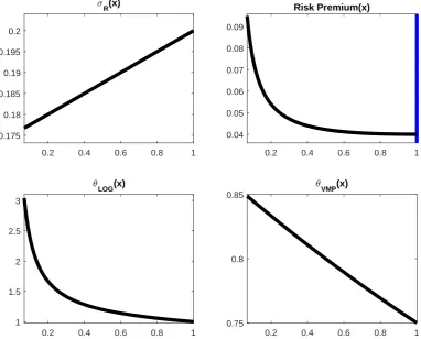
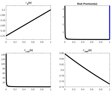
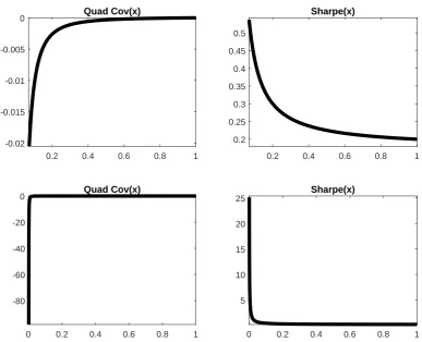
Insert Figure 1.1
Insert Figure 1.2
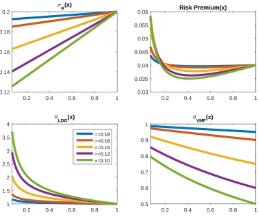
Figures 1.1 and 1.2 offer a convenient graphical representation of my results. Whereas Figure 1.2 plots the equilibrium quantities of interest over the entire state space, Figure 1.1 excludes the region that is in the immediate vicinity of the lower boundary of the state space. Therefore, Figure 1.1 is a zoomed-in version of Figure
analyzing my results. It plots the volatility of the risky asset, σR(·), (top-left panel of the figure), the risk premium, (Et(dRt)−rtdt)/dt, (top-right panel), the portfolio choice of the unconstrained investor,θt, (bottom-left panel), and the portfolio choice of the volatility timer, ˜θt, (bottom-right panel) as functions of the state variable of the model, which is the wealth share of the unconstrained investor. The vertical blue line in the top-right panel of the figure passes through the value ofxtthat minimizes the risk premium. Given that in my calibration the risk premium is decreasing in
xt over the entire state space, the blue vertical line passes through xt = 1.
In the figures, the volatility is increasing in xt over the entire state space (top-left panels). Whereas states in which the unconstrained investor owns most of the wealth in the economy are high-volatility states, those in which the volatility timer owns most of the wealth in the economy are low-volatility states. This result is intuitive. In states in which the volatility timer owns most of the wealth in the economy, volatility should be low in order to induce her to take a large risky asset position and the market for the risky asset to clear. Given that the volatility timer maintains a leverage ratio below one over the entire state space (bottom-right panel), the unconstrained investor is indispensable for market clearing. For the undercapitalized unconstrained investor to be willing to invest in the risky asset and for the market to clear, the risk premium has to be very high in the vicinity of the lower boundary of the state space (top-right panel). In the other extreme, wherextis close to the upper boundary of the state space, the unconstrained investor occupies the driving seat and the effect of the volatility timer in the price formation process is very limited. This is because for high values of xt, the wealth of the volatility timer is small, and this limits the size of the risky asset position she can take. The effective risk aversion of the unconstrained investor decreases as her wealth increases. Consequently, in this region of the state space, the agent is content with holding the risky asset even if the risk premium is relatively low.
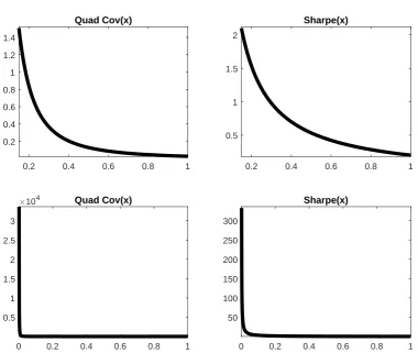
quadratic covariation between volatility and the risk premium.
Insert Figure 1.5
In this particular calibration of the model, the parameter restriction A2 ≤ 1 is
satisfied and the quadratic co-variation takes negative values over the entire state space (please see the top-left and bottom-left panels of the figure). In other words, conditional volatility and expected returns move in the opposite direction. When volatility rises, the risk premium decreases and vice versa. Consequently, any trad-ing strategy that is consistent with the principles of volatility timtrad-ing constitutes a profitable trading strategy. This is because increases in volatility are not fol-lowed by corresponding increases in the risk premium and the risk-return trade-off, as measured by the Sharpe ratio (top-right panel of Figure 1.5), deteriorates in high-volatility states. This is particularly true, when the share of the industry that follows a volatility-managed strategy, ˜Wt/St, is large relative to the total size of the economy, St.
1.4.1. Comparative Statics
Here, I conduct a comparative statics exercise. In particular, I examine how the equilibrium quantities of interest react to changes in the exogenous parameters of the model.
Insert Figure1.10
Insert Figure1.11
Figure 1.11 and the zoomed-in version of that figure in Figure 1.10 plot the sensitivities of conditional volatility, the risk premium, and the portfolio choice to the tightness of the risk limit, ¯σ. A decrease in ¯σ tightens the volatility budget of the volatility-managed portfolio. As a result of this, both the conditional volatility and the leverage ratio of the volatility-managed portfolio decrease over the entire state space. Given that for low values of ¯σ the volatility timer can take smaller risky asset positions (compared to the case in which ¯σ is high), volatility should decrease more in the region of the state space, where the unconstrained investor is undercapitalized, so that the volatility timer can take a large enough risky asset position and the market for the risky asset to clear.
1.5.
Analysis of Equilibrium for
ρ < ρ
vThe model that I develop here allows for rich equilibrium dynamics. For the case in which the consumption-to-wealth ratio of the unconstrained investor is lower than the fund management fee that the volatility-managed portfolio charges, ρ < ρv, the model delivers equilibrium dynamics that are consistent with the predictions of standard heterogeneous agent models. Namely, under this parameter restriction, the conditional volatility implied by my model is positively correlated with expected returns over the entire state space.
The consumption-to-wealth ratio is a good proxy for the degree of patience. An agent with a high consumption-to-wealth ratio admits the interpretation of an im-patient agent. On the other hand, an agent with a low consumption-to-wealth ratio admits the interpretation of a patient agent. Using this terminology, the parametric restrictionρ < ρv is likely to hold in a market environment, where the unconstrained investors are more patient than are the volatility-managed portfolios.
It is instructive to compare the equilibrium implied by my heterogeneous agent model featuring volatility timers to the equilibrium implied by a heterogeneous agent economy devoid of agents engaged in volatility timing. Below, I refer to the latter economy as the baseline economy (model). This comparison is useful, because the baseline economy very much resembles the economic setup in Longstaff and Wang
(2012), a widely cited and standard heterogeneous agent model.
To fill the void resulting from the removal of the volatility timers, I augment the baseline model by adding a new type of agent. In the interest of simplicity, I implicitly characterize the new agent through her portfolio choice, θCM,t,
θCM,t = 1
γCM
µR(xt)−rt
σ2 R(xt)
,
where the abbreviation in the subscript, CM, stands for model of comparison and
is as comparable as possible to the volatility-managed portfolio,
˜
θt= 1 ˜
λt
µR(xt)−rt
σ2 R(xt)
= ¯σ
σR(xt)
,
where ˜λt
.
= λt/σ¯2, and λt is the Lagrange multiplier associated with the volatility budget. Please see the mathematical Appendix for a closed form expression for λt. Whereas the volatility-managed portfolio, ˜θt, is insensitive to the risk premium, the newly defined portfolio, θCM,t, is a function thereof. In other words, the agent that augments the baseline model internalizes the risk-return trade-off at the portfolio construction stage. This is the main point of difference between the new agent and the volatility timer. Notably, θCM,t resembles a mean-variance portfolio. I opt for this particular parametrization in order to enhance the comparability between the volatility-managed portfolio andθCM,t. In the proposition that follows, I summarize the main equilibrium quantities of interest that the baseline model implies. Please refer to the mathematical Appendix for a detailed proof of the proposition.
Proposition 7. (Equilibrium, Baseline Model)
The portfolio choice of the unconstrained investor, the volatility of the risky asset, the
risk premium, and the quadratic co-variation between the risk premium and volatility
in the baseline model are given by
• Portfolio choice of the unconstrained investor
θt=
γCM 1 +xt(γCM −1)
,
• Volatility of the total return process
σR(xt) = σD(1−xtA˘)
1 +xt(γCM −1) 1 +xt(γCM −1)−xtγCMA˘
,
where
˘
A = 1− ρ
ρCM
• Risk premium
Et(dRt−rtdt) =
γCM 1 +xt(γCM −1)
σR2(xt)dt,
• Quadratic co-variation between the volatility of the risky asset and the risk
premium
dhRP(x), σR(x)it= Ψ1(xt)Ψ2(xt)dhx, xit,
where
Ψ1(xt)
.
=− γCM(γCM −1)
(1 +xt(γCM −1))2
σR2(xt) +
2σR(xt)γCM 1 +xt(γCM −1)
Ψ2(xt), Ψ2(xt)
.
=−σDA˘B˜+
γCMA˘A˜
(1 +xt(γCM −1)−xtγCMA˘)2
,
˜
A=.σD(1−xtA˘), ˜
B =. 1 +xt(γCM −1) 1 +xt(γCM −1)−xtγCMA˘
, dhx, xit =((θt−1)σR(xt)xt)2dt.
volatility.
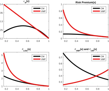
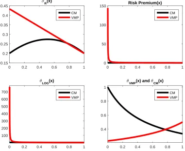
Insert Figure 1.3
Insert Figure 1.4
In all panels, the equilibrium quantities implied by the heterogeneous agent model featuring volatility timers are in red. The equilibrium quantities implied by the baseline model described in Proposition 7 are in black. For ease of interpre-tation, in Figure 1.3, I plot the results for x ∈ [0.15,1]. In Figure 1.4, I plot the results over the entire state space.
It is instructive to compare the equilibrium quantities implied by the model fea-turing volatility timers to the equilibrium quantities implied by the baseline model. The baseline model implies a hump-shaped volatility. Whenxt is close to the lower and upper boundaries of the state space one type of agent dominates, the leverage in economy is low, and volatility is subdued. In the baseline model, the portfolio policies of the agents of the model are positively correlated, and the logarithmic in-vestor takes lower leverage in the vicinity of the lower boundary of the state space, compared to the model featuring volatility timers. Finally, the risk premium im-plied by the baseline model is not very sensitive to the state variable of the model. This is because the two types of agents that populate the baseline economy are very similar. Given that the newly added agent in the baseline economy is slightly more risk averse than the unconstrained investor, the risk premium in the baseline model increases for low values of xt.
most of the wealth in the economy. Her risky asset demand becomes less sensitive to changes in wealth, and this dampens volatility. Similarly, the risk premium is high for low values of xt in order to induce the unconstrained investor to increase her leverage and for the market for the risky asset to clear. For ρ < ρv, high-volatility states are also high risk premium states. An investor willing to support market prices in high-volatility states of the world has the opportunity to earn a high risk premium. The sign of the quadratic co-variation (see Figure1.6) supports this result.
Insert Figure 1.6
1.6.
Broader Perspective and Discussion
In this section, I revisit some of the most important theoretical results from the previous sections and put them in a broader context. In particular, I will argue that, in some special cases, some of my theoretical results are broadly consistent with what standard homogeneous agent general equilibrium models predict. I then compare my results against the main implications of Moreira and Muir (2017) and
Moreira and Muir(2016).
1.6.1. Implications of Homogeneous Agent General Equilibrium Models
A wide range of consumption-based general equilibrium asset pricing models, such as the homogeneous agent economies in Campbell and Cochrane(1999) andBansal and Yaron (2004) and the intermediary asset pricing framework of He and Krish-namurthy (2013) featuring heterogeneous agents, imply a positive relation between asset volatility and risk premia. For example, inCampbell and Cochrane(1999) and
a result of this, in the above class of models, volatility timing does not constitute a sensible approximation to the optimal trading strategy. In the counter-factual case, where I setρ < ρv, the above results carry over to my heterogeneous agent economy.
1.6.2. Relation to Moreira and Muir (2017)
In a recent paper,Moreira and Muir(2017) empirically show that trading strategies that scale standard asset pricing factors, which are widely used in the empirical cross-sectional asset pricing literature, by realized variance over a one-month horizon deliver high alphas. The authors further claim that in their particular dataset the correlation between future expected returns and conditional volatility is very week. In other words, increases in volatility do not lead to increases in expected returns, or if expected returns go up, the increase is marginal relative to the increase in volatility.
formation process and have a big effect on the Sharpe ratio of the risky asset. As a result of this, the unconstrained investors, the centerpiece of my model, are materially affected by the volatility-managed portfolios.
The implications of my model for the realistic case in whichρ > ρv are consistent with the stylized empirical facts reported by Moreira and Muir(2016).
1.6.3. Relation to Martin (2017)
In a recent paper, Martin (2017) derives a lower bound on the equity premium in terms of SVIX, an implied volatility index calculated from the prices of index options. He shows that the SVIX forecast is positively correlated with subsequent returns. He further shows that a contrarian market timing strategy, using SVIX as a signal, delivers a Sharpe ratio considerably higher than the Sharpe ratio of the market. In essence, the trading strategy in Martin (2017) is the opposite of volatility timing as defined here. A trader following the trading strategy in Martin (2017) would increase his risky asset exposure when implied volatility is high and decrease risky asset exposure when volatility is low. It is important to note, however, that the results in Martin (2017) and Moreira and Muir (2017) are not directly comparable. This is because the two papers use different measures of volatility. Whereas Martin
(2017) uses forward-lookingimpliedvolatility, which is extracted from option prices,
Moreira and Muir(2017) use past realizedvolatility.
Furthermore,Martin(2017) shows that the equity risk premium perceived by an unconstrained rational investor with logarithmic utility who is fully invested in the market is proportional to the risk-neutral variance. The risk-premium implied by my model is
Et(dRt)−rtdt=θtVart(dRt).
VarQt(dRt). For the case in which θt= 1,
Et(dRt)−rtdt=VarQt(dRt).
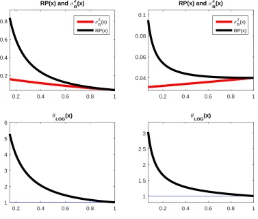
In Figures 1.8 and 1.9, I plot the risk premium (black line) and the variance of the total return process (red line) over the state space.
Insert Figure 1.8
Insert Figure 1.9
In the limit, where the unconstrained investor owns all the wealth in the economy,
xt = 1, θt = 1, and the risk premium is equal to the variance. Over the remaining region of the state space,xt <1, the variance of the risky asset is a lower bound on the risk premium.
1.7.
Conclusion
1.8.
Mathematical Appendix
1.8.1. Portfolio Choice of the Risk-neutral Investor
In this section, I derive the optimal portfolio choice of the volatility-managed port-folio. Here, the main objective is to derive a closed form expression for the Lagrange multiplier, associated with the volatility budget, and express the portfolio choice of the volatility-managed portfolio as a function thereof.
The risk-neutral volatility timer solves the constrained portfolio optimization problem
max
{θ˜t} Et
dW˜t
dt
!
,
s.t. θ˜t≥0,
β
s
Vart(dW˜t)
dt ≤
˜
Wt,
dW˜t = (rtW˜t−C˜t)dt+ ˜θtW˜t(dRt−rtdt).
Given that ˜Ct = ρvW˜t, the SDE for the dynamic budget constraint of the agent takes the form
dW˜t=(rt−ρv) ˜Wtdt+ ˜θtW˜t(µR(·)−rt)dt+ ˜θtW˜tσR(·)dBt. It is then immediate to see that
Et(dW˜t) =(rt−ρv) ˜Wtdt+ ˜θtW˜t(µR(·)−rt)dt,
dhW ,˜ W˜it =(˜θtW˜tσR(·))2dt.
Consequently, Var(dWt) = (˜θtW˜tσR(·))2dt. The corresponding Lagrangian is L= (rt−ρv) ˜Wt+ (µR(·)−rt)˜θtW˜t+λt( ˜Wt−β
q
where λt is the Lagrangian multiplier associated with the risk limit (volatility bud-get). The first order condition with respect to ˜θt gives
˜
θt=
µR(·) ˜Wt−rW˜t
λtβ(˜θtW˜tσR(·))−1
( ˜WtσR(·))−2.
In Proposition3, I prove that the risk premium on the risky asset is positive over the entire state space. Consequently, it is optimal for the risk-neutral agent to increase the size of her risky asset position up to the volatility limit. Therefore, the dynamic constraint holds with equality, i.e.,
β
s
Vart(dW˜t)
dt = ˜Wt.
This allows me to derive an expression for ˜Wt, ˜
Wt=β
µR(·) ˜Wt−rtW˜t
λtβ(˜θtW˜tσR(·))−1
(σR(·) ˜Wt)−1. Additionally, it is useful to note that
(˜θtW˜tσR(·))−1 =
β
˜
Wt
.
The next step is to solve for the Lagrange multiplier,
λt=
µR(·)−rt
βσR(·)
.
I substitute the expression for the Lagrange multiplier into the first order condition, with respect to ˜θt, and after a straightforward simplification I obtain the optimal portfolio policy,
˜
θt = 1
βσR(·)
= σ¯
σR(·)
.
1.8.2. Portfolio Choice of the Unconstrained Investor
In this sub-section of the mathematical Appendix, I derive the optimal portfolio policy of the unconstrained investor, θt, who is endowed with logarithmic utility over instantaneous consumption. I start from the market clearing condition,
θt
Wt
St + ˜θt
˜
Wt
St = 1,
where the constant on the right-hand side is the total supply of the risky asset. Given that I model a pure exchange economy, ˜Wt =St−Wt. Consequently,
θt
Wt
St + ˜θt
St−Wt
St
=1, θtxt+ ˜θt(1−xt) =1.
The last step is to solve the above expression for θt. The optimal portfolio policy of the unconstrained investor,
θt= 1
xt
−1−xt
xt ˜
θt = 1
xt
− 1−xt
xt ¯
σ σR(·)
,
follows immediately.
1.8.3. Price-Dividend Ratio
In this sub-section of the mathematical Appendix, I derive an expression for the price-dividend ratio on the risky asset. I impose market clearing in the consumption goods market,
and note thatCt =ρWt, and ˜Ct=ρvW˜t. Using the fact that ˜Wt =St−Wt, I obtain
ρWt+ρv(St−Wt) = Dt. I then solve the above expression for St and obtain
St= 1
ρv
Dt+
1− ρ
ρv
Wt.
To obtain an expression for the price-dividend ratio divide both sides by Dt,
St Dt =1 ρv +
1− ρ
ρv Wt Dt St St =1 ρv +
1− ρ
ρv
St
Dt
xt.
Solving for St/Dt, I obtain an expression for the price-dividend ratio,
St
Dt
= 1
ρv−xt(ρv −ρ)
.
This completes the derivation of the price-dividend ratio on the risky asset.
1.8.4. Proof of Proposition 1 (Model-Implied Total Return Process Volatility)
I start from the definition of the total return process,
dRt =
Dtdt+dSt
St
.
It is then immediate to see that
µR(·)dt+σR(·)dBt =
Dtdt
St
+ dSt
St
.
Clearly, in order to compute the diffusion coefficient of the total return process,
stochastic differential equation for {St}. I note that ρv and ρ are constants and do Itˆo on
St= 1
ρv
Dt+
1− ρ
ρv
Wt. The stochastic differential equation
dSt= 1
ρv
dDt+
1− ρ
ρv
dWt
follows immediately. I then use the facts that the exogenous dividend process follows a geometric Brownian motion and the stochastic differential equation
dWt=−Ctdt+rtWtdt+θtWt(dRt−rtdt)
governs the intertemporal wealth evolution of the unconstrained investor. The above SDE simplifies to
dSt= 1
ρv
(µDDtdt+σDDtdBt) +
1− ρ
ρv
(rWtdt−Ctdt+θtWt(dRt−rtdt)) =(·)dt+
1
ρv
σDDt+
<