An Improved Numerical Algorithm for the Fractional Differential Equations and Its Application in the Fractional Order Nonlinear Systems

2017 3rd International Conference on Computer Science and Mechanical Automation (CSMA 2017) ISBN: 978-1-60595-506-3

An Improved Numerical Algorithm for the Fractional Differential

Equations and Its Application in the Fractional-Order Nonlinear Systems

Xiang-Jun WU

and Bao-Qiang LIU

1_{College of Software, Henan University, Kaifeng475004, P. R. China} 2

School of Computer and Information Engineering, Henan University, Kaifeng 475004, P.R. China

Email: [email protected], [email protected]

Keywords: Fractional order, Improved numerical algorithm, Variationaliteration, Synchronization.

Abstract. In this paper, an improved numerical algorithm for the fractional differential equations is proposed based on the variational iteration method. Using the improved numerical scheme, we investigate a new fractional-order hyperchaotic system, and find that hyperchaos does exist in the new fractional-order four-dimensional system with order less than 4. The lowest order we find to yield hyperchaos is 3.46 in this new fractional-order system. The existence of two positive Lyapunov exponents further verifies our results. Numerical results show that the proposed method has a faster speed and more accurate comparing with the traditional predictor-corrector algorithm. Based on the stability theory of the fractional-order system, a nonlinear controller is constructed to achieve synchronization fora class of nonlinear fractional-order systems using the pole placement technique. The nonlinear control method can synchronize two different fractional-order hyperchaotic systems. This synchronization scheme which is simple and theoretically rigorous enables synchronization of fractional-order hyperchaotic systems to be achieved in a systematic way and does not need to compute the conditional Lyapunov exponents. Simulation results are given to validate the effectiveness of the proposed synchronization method.

Introduction

Although fractional calculus is a 300-year-old mathematical topic, fractional calculus starts to attract increasing attention of physicists and engineers from an application point of view [1, 2]. It was found that many systems in interdisciplinary fields can be elegantly described with the help of fractional derivatives. For example, The electrode-electrotype interface is a sample of fractional-order processes because at metal-electrolyte interfaces the impedance is proportional to the non-integer order of frequency for small angular frequencies [3]. The resistance-capacitance-inductance interconnect model of a transmission line is a fractional-order model [4]. In the fractional capacitor theory, if one of the capacitor electrodes has a rough surface, the current passing through it is proportional to the non-integer derivative of its voltage [5]. In economy, it has been known that some finance systems can display fractional order dynamics [6]. More examples for fractional-order dynamics can be found in [2]. Moreover, applications of fractional calculus have been reported in many areas such as signal processing [7], automatic control [8] and robotics [9]. So it is important to investigate the dynamical systems with fractional-order models.

However, there are many material differences between the ordinary differential equation systems (integer-order) and the corresponding fractional-order differential equation systems. Most of the properties or conclusions of the integer-order system cannot be simply extended to the case of the fractional-order one. To date, it was found that many fractional-order differential systems such as the fractional-order Rössler system [10], the fractional-order Chen system [11], the fractional-order Lü system [12], the fractional-order unified system [13] etc, display chaotic behavior.

addition, the predictor-corrector algorithm for solving the fractional differential equations requires more computational complexity, which leads to a slow running speed. The computational precision of it is unsatisfactory. Motivated by the above discussions, in our work, we present an improved numerical algorithm for the fractional differential equations. By the proposed numerical algorithm, we numerically investigate the hyperchaotic behaviors of a novel fractional-order four-dimensional system. It is found that hyperchaos indeed exist in the new fractional-order system with order as low as 3.46. The hyperchaotic dynamical behaviors of the system were demonstrated by computer simulations. Numeric evidence shows that the proposed algorithm is superior to the current predictor-corrector algorithm. Furthermore, synchronization of the fractional hyperchaotic systems is also investigated.

Fractional Derivative and the Improved Numerical Algorithm

There are some definitions for the fractional differential operators [1]. Riemann-Liouville definition is commonly used and defined by

d

( ) ( ), 0 d

n n n

D x t J x t

t

α −α _α

= > _{, (1)}

wheren=_{  }α _{, i.e.,} n is the first integer which is not less than α_, Jβ is the β_-order Riemann-Liouville integral operator as described by

1 0

1 ( )

( ) d , 0 1

( ) ( )

t

J t

t

β

β

φ τ

φ τ β

β τ −

= < ≤

Γ

∫

whereΓ ⋅( ) _{is the gamma function.}

Here and throughout, only the following definition is applied:

( )

( ) n n ( ), 0 D x tα J −αx t α

∗ = > , (3)

where n=_{  }α _{. The Riemann-Liouville fractional derivative appears unsuitable to be treated by the} Laplace transform technique in that it requires the knowledge of the non-integer order derivatives of the function at t=0 _{[14]. This problem does not exist in the Caputo definition that is sometimes}

referred as smooth fractional derivative in literature [15]. In addition, Riemann-Liouville initial problems require homogeneous initial conditions, whereas Caputo initial problems allow us to specify inhomogeneous initial conditions too if this is desired [16]. It is known [17] that under those homogeneous conditions the problems with Riemann-Liouville operators are equivalent to those with Caputo operators. So we would prefer the Caputo derivative to the Riemann-Liouville one.

The numerical calculation of a fractional differential equation is not as simple as that of an ordinary differential equation. Here we choose the Caputo version and use the variational iteration method for fractional differential equations according to the basic ideas in [18, 19]. The following is a brief introduction of the algorithm.

The following differential equation:

( ) ( ) 0 d

( , ), 0 d

(0) , 0 1 2 1

k k

x

f t x t T t

x x k n

α α



= ≤ ≤

 

 _{= =}

 , , ,,

-,

is equivalent to the Volterra integral equation [20]

1 ( )

0 ₀ 1

0

1 ( , ) d ! ( ) ( )

k _t

k k

t f x

x x

k t

α

α

τ τ

α τ

−

   

− =

= +

Γ −

∑

∫

We apply the variational iteration method in the above equation as follows:

1 ( )

1 0 ₀ 1

( , ( )) 1

( ) ( ) d

! ( ) ( )

k _t

k n

n

f x

t

x t x t

k t

α

α

τ τ

τ

α τ

−

   

+ = + −

Γ −

where the initial values (0) (1) ( 1) 1

0( ) 0 0 0

n n

x t =x +x t++x − t− _.

Dynamics of a New Fractional-Order Four-Dimensional System

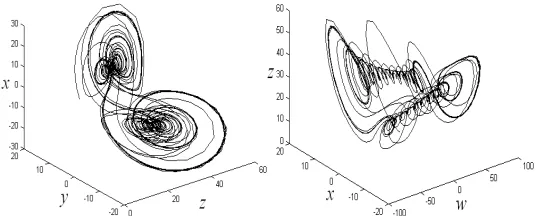
More recently, Gao et al. proposed a new hyperchaotic system [21] by adding a nonlinear quadratic controller to the second equation of the three-dimensional autonomous modified Lorenz chaotic system [22],which is given by

( )

x a y x

y bx y xz w

z xy cz

w dyz

= −



 _{= + − −}



 _{= −}



 =



, (6)

where a, b, c anddare the system parameters. When a=10_{, b}=_28, c=_{8 3 andd}=_{0.1, system (6)} behaves hyperchaotically as shown in Fig. 1.

Now we consider the fractional version of the new hyperchaotic system as follows:

d

( ) d

d d d d d d

x

a y x t

y

bx y xz w

t z

xy cz t

w dyz t

α α α

α α

α α

α 

= −

  

= + − −

 

 _{= −}

 

 ₌



, (7)

where 0<α≤1_.

According to the improved numerical algorithm of the fractional-order system in Section 2, we find that hyperchaos does exist in the new four-dimensional system with fractional order. In the following simulations, the system parameters are always chosen as a=10, b=28, c=8 3 andd=0.1

.The simulation results demonstrate that hyperchaos indeed exists in the fractional-order system (7) with order less than 4. Numeric evidence shows that, when 0.865183290824756≤α≤1, the fractional-order system (7) always exhibits hyperchaotic behaviors. For instance, when α =0.94_, α =_0.92and

0.865183290824756

α = _{, hyperchaotic attractors are found and the phase portraits are depicted in Figs.} 2, 3 and 4, respectively. The two largest Lyapunov exponentsλ1,λ2of the simulation time series are

obtained as follows:(i)when α =0.94_,

1 1.2635

λ = _and

2 0.9432

λ = _{; (ii)when}α =_0.92,

1 1.0829

λ = _and

2 0.8752

λ = _{; (iii)when}α =_{0.865183290824756,}

1 0.823

λ = _and

2 0.026

λ = _{. Obviously, the fractional-order} system (7)is hyperchaotic. However, when α <0.865183290824756_{, the fractional-order system (7)has}

no hyperchaos. The phase portraits of system (7) for α =0.864 _{are shown in Fig. 5. System (7) does}

not display hyperchaotic, but limit cycles appear which implies that there is no hyperchaos in the fractional-order system (7). Therefore, the lowest limit of the fractional order for this system to be hyperchaoticisα =0.865 0.864− _{. Thus, the lowest order we found for this system to yield hyperchaos} is 3.46.

Figure 1. Hyperchaotic attractors of the new system (6).

Figure 2. Hyperchaotic attractors of the fractional-order hyperchaotic system (7) with α=0.94.

Figure 3. Hyperchaotic attractors of the fractional-order hyperchaotic system (7) with α=0.92.

Figure 4. Hyperchaotic attractors of the fractional-order hyperchaotic system (7) with

0.865183290824756

Figure 5. Phase plots of the fractional-order system (7) withα=0.864.

Table 1. Comparion of the performance of the proposed algorithm and the predictor-corrector algorithm.

Algorithm Average running time _(Second) the lowest order for yield _hyperchaos

Our improved algorithm 28 α=0.865183290824756

The predictor-corrector algorithm 130 α ≈0.916

The Controller Design based on the Stability Theory of Fractional-Order System

Consider the following fractional-order system described by

d

( )

dt f

α

α = + +

x

Ax B x C, (8)

where n

R ∈

x is a n-dimensional state vector of the system, n n

R×

∈

A , n n

R×

∈

B and n

R ∈

C are constant matrices, f( ) :x Rn→Rn is a nonlinear vector function in terms of x, and 0<α≤1 _{is the fractional}

order. Axis the linear part of the system (8) and Bf( )x is the nonlinear part. System (8) is regarded as a drive system. Many fractional-order chaotic systems can be described as the form of system (8).

Introduce an additive controller n

U∈R _{, then the controlled response system is given by}

d

( )

dt g U

α

α = ′ + ′ + +

y

A y B y D . (9)

where n

R

∈

y denotes the state vector of the response system, n n

R×

′ ∈

A , n n

R×

′ ∈

B and n

R

∈

D are matrices of this controlled response system parameters, and ( ) : n n

g _y R →R _{is a smooth nonlinear}

function. If _{A = A}′_{, B = B}′_, C=D and f( )_x =g( )_{x , thenx and y are the states of two identical}

fractional-order systems. Otherwise, x and y are the states of two different fractional-order systems.

The synchronization problem is to design a suitable controllerU, which synchronizes the states of both the drive and response systems. For this end, the synchronization error between system (8) and system (9) is defined as_{e = y}−_{x.The fractional-order synchronization error system can be written as} follows:

d

( ) ( )

d

( ) ( ) ( )

g f U

t

g f U

α

α = ′ + ′ + − − − +

′ ′ ′

= + − + − + − +

e

A y B y D Ax B x C

A e B y B x A A x D C

. (10)

Various choices of the controller are possible. Here, we choose the controller as

( ) ( ) ( )

U =Bf x −B′g y + A−A x C′ + −D−Ke. (11)

d

( )

dt

α

α = ′−

e

A K e. (12)

We can obtain the following theorem.

Theorem 1.According to the stability theory of fractional-order systems, global asymptotic chaos synchronization between the fractional-order drive system (8)and the response system (9) can be obtained by choosing K such that | arg( (λi A′ −K)) | 0.5> απ (i=1, 2, 3, 4) wherearg( (λi A′ −K)) denotes the

argument of the eigenvalue λi of (A′ −K) in Eq. (12).

If the pair (_{A I}′, ) _{is controllable, from linear control theory, it follows that the eigenvalues of} (_A′ −_K) _{in system (12) can be placed anywhere by proper choice of the gain}

i

k (i=1, 2, 3, 4)_{and then}

there surely exist ki (i=1, 2, 3, 4) such that | arg( (λi A′ −K)) | 0.5> απ (i=1, 2, 3, 4) .The solution to the

problem of determining K such that the arguments of all the eigenvalues (or poles) of the matrix

(_A′ −_K) _{in Eq. (12) satisfy | arg( ( )) | 0.5} i

λ A′ −K > απ, i.e., the fractional-order drive system (8) and the fractional-order response system (9) is in a state of asymptotic synchronization can be easily obtained by the pole placement technique from control system theory such as the Ackermann’s method.

In the following, we will validate the proposed scheme via a numerical example. The drive system is given as system (13). The fractional-order Chen hyperchaotic system (14) is used as a response system.

1

1 1 1

1

1 1 1

1 1 1

1

1 1 1

1 d

d

0 0 0 0 0 0

d

1 0 1 0 1 0 0

d

0 0 0 1 0 0 0

d

0 0 0 0 0 0 0

d d

d x t

x x y

a a

y

y x z

b t

c z y z

z

d

w z w

t w t α α α α α α α α       −                     − _{ } − _{ }     = +        −                _{   }            

, (13)

2

1

2 2 2

2

2

2 2 2

3

2 2 2

2

2 2 2 4

2 d

d

0 1 0 0 0 0

d

0 0 0 1 0 0

d

0 0 0 1 0 0 0

d

0 0 0 0 0 1 0

d d d x t u

x x y

y

u

y x z

t

u

z y z

z

w z w u

t w t α α α α α α α α θ θ β γ δ λ       −                         _{ } − _{   }     = + +          −                  _{       }        

, (14)

where θ =35_, β =_7, γ =_{12 ,} δ =_{3 and} λ =_{0.5. When 0}

i

u = _(i=_{1, 2, 3, 4)and} α =_{1, Eq. (14) is the} classical integer-order Chenhyperchaos equation, and it has a hyperchaotic attractor. When ui=0

andα∈[0.93,1]_{, it has a hyperchaotic attractor.}

From systems (13) and (14), the following error dynamical system can be obtained:

1

1 2 2 1 1

2

2 2 2 1 1

3 2 2

3 2 2 4 4 d d

0 1 0 0 0 0 0 0 0 0

d

0 0 0 1 0 0 0 1 0 0

d

0 0 0 1 0 0 0 1 0 0 0

d

0 0 0 0 0 1 0 0 0 0

d d

d e t

e x y x y

e

e x z x z

t

e y z y

1 1 2 1 3 1 1 4 0 1

1 0 1

0 0 0

0 0 0

u x a a u y b u c z w u θ θ β γ δ λ − −            _{− −}        + +      −             

. (15)

where e1=x2−x1, e2= y2−y1, e3=z2−z1 and e4=w2−w1.

According to Eq. (11), the controller can be constructed as:

1 1 1 2 2

2 1 1 2 2

3 1 1 2 2

1 1 2 2

4

0 0 0 0 0 0 0 0

0 1 0 0 0 1 0 0

1 0 0 0 1 0 0 0

0 0 0 0 0 1 0

u x y x y

u x z x z

u y z y z

d z w z w

u            ₋    ₋    =  −                           1 1 2 1 3 1 1 4 0 1

1 0 1

0 0 0

0 0 0

e x a a e y b e c z w e θ θ β γ δ λ − −            _{− −}        − −      −             

K . (16)

Substituting Eq. (16) in Eq. (15) gives

1 1 1 2 2 2 3 3 3 4 4 4 d d 0 1 d 0 0

d _{( )}

0 0 0

d

0 0 0 d d d e t e e e e e t e e e e e t e t α α α α α α α α θ θ β γ δ λ       −                       ′ = − = −        −            _{   }          

K A K e. (17)

In the following simulation, the parameters are always selected as a=10_{, b}=_{28, c}=_{8 3,d}=_0.1,

35

θ = _, β =_7, γ =12 _, δ =_{3 and} λ =_{0.5. The fractional order} α _{is set as} α=_{0.95. Both the new}

fractional-order system (6) and the fractional-order Chen system (14) are hyperchaotic. The initial states of the drive system (13) and the response system (14) are taken as(10, 10, 7, 8)− _{and( 8, 6, 8, 5)}− − − _,

respectively. From Eq. (17), it is obvious that the pair (_{A I}′, ) _{is controllable. Thus, the condition} | arg( (λ_i A′ −K)) | 0.5> απ can be satisfied for arbitrary λ_i(A−K)= −[ 2 −2 −2 −2](i=1, 2, 3, 4)_{.Applying the}

pole placement technique, we have

33 35 0 1 7 14 0 0

0 0 1 0

0 0 0 2.5

−       =  −      K .

tt

(a) Time response ofx1( )t (―) and x2( )t (--)(b) Time response ofy1( )t (―) and y2( )t (--)

tt

(c) Time response ofz1( )t (―) andz2( )t (--)(d) Time response ofw1( )t (―) andw2( )t (--)

t

(e) Synchronization errors

Figure 6.Simulation results of synchronization between system (13) and system (14) with α=0.95.

Conclusions

This paper proposes an improved numerical algorithm for the fractional differential equations based on the variational iteration method. Using the presented algorithm, the hyperchaotic behaviors of a new fractional-order four-dimensional system are numerically studied. We have found that hyperchaos does exist in the new fractional-order system with order as low as 3.46. The hyperchaotic dynamical behaviors of the system are illustrated by computer simulations. Numerical results demonstrate the proposed numerical algorithm is superior to the traditional predictor-corrector scheme. Further, based on the stability theory of the fractional-order system, the nonlinear controller is designed to achieve synchronization for a class of nonlinear fractional-order systems by employing the pole placement technique. The synchronization method is rather simple, theoretically rigorous and convenient to implement in practice, and does not require computing the conditional Lyapunov exponents. For verifying the effectiveness of the presented synchronization scheme, some numerical simulations are performed in our work.

Acknowledgment

and 2015T80396), Program for Science & Technology Innovation Talents in Universities of Henan Province, China (Grant No 14HASTIT042), the Foundation for University Young Key Teacher Program of Henan Province, China (Grant No 2011GGJS-025), Shanghai Postdoctoral Scientific Program (Grant No 13R21410600).

References

[1]I. Podlubny, Fractional differential equations. Academic Press, New York, 1999.

[2]R. Hifer, Applications of fractional calculus in physics. World Scientific, New Jersey, 2001.

[3]M. Ichise, Y. Nagayanagi, T. Kojima, J Electroanal Chem, 33, 253-265, 1971.

[4]G. Chen, G. Friedman, IEEE Trans. Comput. Aided Des. Integr. Circuits Syst, 24, 170-183, 2005.

[5]R. De. Levie, J Electroanal Chem, 261, 1-9, 1989.

[6]N. Laskin, Physica A, 287, 482-492, 2000.

[7]B. Mandelbrot, J.W. Van Ness, SIAM Rev, 10, 422-437, 1968.

[8]I. Podlubny, IEEE Trans. Automat Control, 44, 208-214, 1999.

[9]F. B.M. Duarte, J.A.T. Macado, Nonlinear Dyn, 29, 315-342, 2002.

[10]C.G. Li, G. Chen, Physica A, 341, 55–61, 2004.

[11]C.G. Li, G. Chen, Chaos Solitons & Fractals, 22, 549-554, 2004.

[12]J.G. Lu, Phys Lett A, 354, 305-311, 2006.

[13]X. Wu, J. Li, G. Chen, J Franklin Institute, 345, 392-401, 2008.

[14]S.G. Samko, A.A. Klibas, O.I. Marichev, Fractional integrals and derivatives: theory and applications. Gordan and Breach, Amsterdam, 1993.

[15]M. Caputo, Geophys. J R Astron Soc, 13, 529-539, 1967.

[16]F. Keil, W. Mackens, J. Werther, Scientific computing in chemical engineering II-computational fluid dynamics, reaction engineering, and molecular properties. Springer-Verlag, Heidelberg, 1999.

[17]P. L. Butzer, U. Westphal, An introduction to fractional calculus. World Scientific, Singapore, 2000.

[18]L. Xu, Comput Math Appl, 54, 1071-1078, 2007.

[19]A. Ghorbani, J.S. Nadjufi, Nonlinear Anal RWA, 10, 2828-2833, 2009.

[20]K. Diethelm, N.J. Ford, J Math Anal Appl, 265, 229-248, 2002.

[21]T. Gao, G. Chen, Z. Chen, S. Cang, Phys Lett A, 361, 78-86, 2007.