User’s Gender Prediction Based on Smartphone Applications Installed: Analysis from Real World Data to Simulation

2017 2nd International Conference on Computational Modeling, Simulation and Applied Mathematics (CMSAM 2017) ISBN: 978-1-60595-499-8

User’s Gender Prediction Based on Smartphone Applications Installed:

Analysis from Real World Data to Simulation

Wen-yi FU

, Chen-yu MA, Quan-neng HUANG and Xian-kai WANG

Trustdata, Poly International Plaza, Chaoyang District, Beijing, China

Keywords: Gender prediction, Smartphone applications, Simulation.

Abstract. Users’ gender information for a smartphone application cannot be approached directly

since it is considered as private. However, this basic demographic information is of great value during persona analysis. In this paper, an innovative feature selection approach is proposed for gender prediction based on smartphone applications installed. We construct weighted average female-oriented and male-oriented features, and applying it to four machine learning algorithms. Meanwhile, simulation is carried out to make horizontal models comparison easy even between supervised and unsupervised algorithms. Prediction accuracy can be as high as 90.4% for weighted average logistic regression model.

Introduction

Gender is a crucial feature when during persona analysis. For enterprises, they can carry out users behavior analysis and targeted advertising by associating gender and other demographic information. For mobile app developers, knowing the sex ratio of users can help strengthen or improve using experience. However, due to the privacy protection, it is impossible to know each user's gender during information collection. Predicting the sex of the user through the user's open behavior information and resources will be of great value.

With over 160,000 users’ mobile application installation package lists, we plan to predict by including users gender ratio of applications. This paper solves this problem by introducing related previous work in Chapter 1, and stating analysis objective in Chapter 2, then constructing effective characteristic variables, proposing four machine learning algorithms in Chapter 3. In Chapter 4, data simulation and validation will be used for the first time to evaluate model performances for both supervised and unsupervised learning algorithms. Eventually, Chapter 5 we select the best technique by comparing evaluation metrics and drawing conclusions. The technique discussed in this paper will deepen the level of information that is available to be analyzed.

Related Work

Some papers did the same kind of prediction based on mobile applications. Seneviratne et al. (2015)[1] monitoring the application of mobile phones installed by 174 android users, the gender was predicted by logistic regression model with 69.8% accuracy. After that, Eric (2016)[2] used the same logistic regression, but he increased the sample size to 3760 and only analyzed apps of used at least once a month. This model reached 82.3% accuracy. Eric’s proved that the model accuracy is proportional to the sample size. D. Kelly et al. (2015)[3] makes gender prediction based on the user's mobile phone applications’ keywords and the feedback of users social networks.

the user access to web pages that disclose users preferences and interests. Z Qin et al. (2016)[8] took advantage of the connection between user demographic information and requests of network resources, proposing naïve Bayesian, decision tree model and logistic regression models. And do feature smoothen for similar users at the final stage of prediction, improve the probability of correctly predict users gender.

Dataset and Objective

Two different datasets contained over 160,000 Chinese android users’ mobile applications installation. One is the 100,000 sample users with gender unknown, and the other is 63163 users with labeled gender. The goal of this paper is to try predicting the gender for unlabeled data as accurate as possible.

138566 distinct mobile applications installed for all sampled users (including the system applications), and 99.72 applications installed per user on average. We got top 41 mobile phone applications with highest amount of installation and their corresponding proportion of male users.[9] The top 10 apps in the sample dataset with the highest amount of installation are: Taobao, Changba, Wifi-locating, Meituan, Glory-of-the-king, Gif-maker, Meitu and Jingdong. The top 10 apps with the highest proportion of female users are: Dayima, Miya, Meijialove, Meiyan-camera,Ttpic, Boohee, Meituan and Meituxiuxiu. The top 10 apps with the highest proportion of male users are: Huya-liveshow, Douyu-liveshow, e-daijia, Panda-liveshow, Auto-home, Guazi-dealer, Ludashi, Fantancy-westward-journey, YY-liveshow and Lu-fax.

Prediction Based on Different Learning Algorithms

Feature Selection

Users are telling his/her gender by installing gender-oriented applications. The key to our characteristic variables is to choose representative applications as features. The more typical an application is, the more information it gives. Thus, applications with gender proportion away from 50% will be strong gender-oriented applications which could be our feature variable candidates.

Also, a balance between female-oriented and male-oriented applications is important in feature selection to get a stable and unbiased prediction. It is a balance of the number of variables chosen for each kind of gender oriented applications, also the prevalence of them.

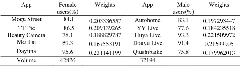
Under these rules, ten applications are chosen (Table 1). They are divided evenly into two parts. The users’ gender proportion is at least 60% and is as high as 90%. The proportion of amount of installed is 1:1.3. Therefore, features are selected and ready to be transferred into characteristic variables.

For each application, if a user installed this application, we assume that the probability of a user is male equals to this application’s proportion of male users. Otherwise, it equals to the proportion of female users. Denote p_ij as the ith user’s probability of being male, AppP_j as the proportion of male users for the jth application.

p_ij = AppP_jΙ_instij + (100 − AppP_j) (1 − Ι_instij)

Ι_{𝑖𝑛𝑠𝑡𝑖𝑗} = { 1, if the ith users installed the jth application 0, if the ith users didn′tinstall the jth application

The corresponding pseudo codes to achieve above equations are as follow: For user in Users:

Feature_Installed = [1 if installed apps in feature applications else 0 for installed apps in all other apps]

For i in feature applications: If Feature_installed == 1:

Else:

Prob[i] = the ith application female users proportion

However, the level of entropy each application carries will be ignored. We proposed weighted average gender probability as our characteristic variables, in order to bring higher variance between applications.

Table 1. Gender oriented applications.

App Female

users(%)

Weights App Male

users(%)

Weights

Mogu Street 84.1 _{0.203336557 Autohome 83.1 0.197293447}

TT Pic 86.5 0.209139265 YY Live 77.6 0.184235518

Beauty Camera 78.1 0.188829787 Huya Live 93.3 0.221509972

Mei Pai 69.3 0.167553191 Douyu Live 91.4 0.21699905

Dayima 95.6 0.231141199 Qiushibaike 75.8 0.179962013

Volume 42826 32194

For the jth application, the weight (wj) is expressed in Eq. 1.

w_j = AppPj

∑mj=1AppPj

, j = 1,2, … ,10 (1)

Therefore, for the ith user, the probability of being female (fi) and male (mj) are expressed in Eq.

2.

fi = ∑m/2j=1 wj(100 − pij)Ι𝑖𝑛𝑠𝑡𝑖𝑗 ; mi= ∑ wjpijΙ𝑖𝑛𝑠𝑡𝑖𝑗

m i=m

2+1

(2)

Weighted Average Clustering

Unsupervised learning algorithms can be applied to our unlabeled data, Clustering is one of them. Cluster analysis is not a specific algorithm. It contains several models. The basic steps of K-means algorithm is to randomly initialize the center of clusters, then attribute the closest cluster to each data point, then set the position of each cluster to the mean of all data points belonging to that cluster, and we need to repeat the previous steps until centers convergence.

We optimize cluster models by controlling the expected number of clusters. Models evaluated by two index: Silhouette Coefficient and MSE.

Silhouette Coefficient[11]: for each data point a, let a(i) be the average dissimilarity of i with all other data within the same cluster, and b(i) be the lowest average dissimilarity of i to any other clusters, of which i is not a member. Silhouette coefficient can be defined as Eq. 3.

S = 1

n∑

b(i)−a(i) max{a(i),b(i)} n

i=1 ∈ [−1,1] (3)

Silhouette coefficient ranges from -1 to 1. The closer it to 1, representing more coherent within cluster and separate between clusters, which is what we want for well-separated clusters. Thus, we are going to find model that has Silhouette coefficient close to 1.

Mean Square Error (MSE): Since the gender proportion of each application is known, the predicted gender proportion can also be calculated from the predicted gender of each user. When the predicted genders are accurate, the difference between true and predicted gender proportion should be really small. Therefore, we proposed mean square error (MSE) to evaluate how far our predicted ratio from true gender ratio. It can be defined as Eq. 4.

MSE =1

n∑ (true ratioi− predicted ratioi) 2 n

i=1 (4)

The corresponding pseudo codes to return the best number of clusters are as follow: F = np.average(female_feature_installed,weights=female_weight)

M = np.average(male_feature_installed,weighted=male_weight) Avg = list(zip(f,m)

Def sh_score(min_k,max_k): Sh_score = []

For I in range(min_k,max_k):

Cluster_labels = KMeans(n_cluster=k,init=“k-means+”).fit(avg).labels_ Sh_score.append(silhouette_score(features,labels))

Best_cluster = min(list(enumerate(sh_score,start=min_depth)) Return(best_cluster)

After calculation, the optimal expected number of cluster is k = 3, which is going to maximize Silhouette coefficient and minimize MSE.

Diagonal Classifier

We got two variables, one is the probability of a user is female, and the other is the probability of being male. By common logic, we deduce a rule to classify user’s gender: user belongs to a gender which this user has a higher probability. Since it is a linear classifier with slope=1, we name this classification algorithm as diagonal classifier.

The corresponding pseudo codes to achieve diagonal classifier are as follow: F = np.average(female_feature_installed,weights=female_weight)

M = np.average(male_feature_installed,weighted=male_weight) For user in Users:

If f>m:

Gender = ‘female’ If m>f:

Gender = ‘male’ Else:

Gender = ‘unknown’

Decision Tree

The philosophy of decision tree algorithm is based on the successive division of the problem into several subproblems with a smaller number of dimensions, until a solution for each of the simpler problems can be found.[12] Because the decision branch is graphically shaped like a tree trunk, it is called a decision tree. In machine learning, decision tree is a predictive model, which represents a mapping relation between object attributes and object values. The nodes are divided by Gini impurity.

The maximum depth of tree is controlled to optimize models. Labeled dataset is split into train set and test set, and models evaluated by accuracy for each maximum depth. The 100,000 unlabeled data can be used as validation set, evaluated by MSE. Ideally, we can find a maximum depth to maximize accuracy and minimize MSE.

The corresponding pseudo codes to achieve decision tree are as follow: Avg = list(zip(F,M)

def best_tree_by_mse(min_depth,max_depth): depth_range = range(min_depth,max_depth) MSE = []

for i in depth_range: MSE.append(mse(i))

gender_tree = tree.DecisionTreeClassifier(max_depth = best_depth).fit(avg,sex) return(best_depth,min(MSE))

Logistic Regression

Since the dependent variable of this case is a binary virtual variable, we can try the logistic regression model. Logistic regression is a generalized linear regression. The difference between ordinary linear regression is that the dependent variable follows the binomial distribution instead of the normal distribution, Y ϵ {0,1}. The model can be expressed as Eq. 5.

Pr(Y=k|X) =β₀+ β₁X₁+ β₂X₂ (5) Parameters are estimated with the maximum likelihood method. Given observation x, we predict y such that (Eq. 6):

ŷ = argmaxPr(Y=k|X=x) (6) If we denote the probability of being male as ‘1’, the response variable is the probability of being male. Users will be classified as male if the response variable exceeds a threshold, otherwise it will be classified as a female. Threshold should be controlled in case of overfitting. Since threshold hasn’t been available to be controlled in Python 3.0, this process can be completed in R by drawing ROC curve.

Models Performance with Simulated Data

Model comparison can be inaccurate because of inaccurate gender proportion of each application provided. A labeled dataset can be simulated with known gender proportion and volume of installation set by us. Accuracy of evaluation within models can be guaranteed in this case.

Data Simulation

Gender proportion and amount of installation of each application need to be set prior to simulation. Assuming that the gender proportion is 1:1 for a large sample size.

pi: male user proportion for the ith application. i = 1,2, … ,10

I_i: amount of installation fot the ith application. i = 1,2, … ,10 No_F_i: the number of female users for the ith application No_M_i: the number of male users for the ith application. n: number of users simulated.

The corresponding pseudo codes to simulate data are as follow: Pop=n

Sex = list('female'*(pop/2)+'male'*(pop/2)) For I in range(i):

No_M = nIp No_F = nI(1 − p)

female_select = random select F numbers from the first half of Sex male_select = randomly select M numbers from the second half of Sex all_select = combine selected female and male

#assign "1" for selected people representing he/she installed this app installed = [1 if num in all_select else 0 for num in range(pop)]

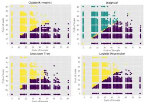
Results

Figure 1. Classification results predicted by K-means (top left), diagonal classifier (top right), decision tree (bottom left) and logistic regression (bottom left).

To show how much the weighted average features improves our models, comparisons between weighted and unweighted feature for each algorithm are also made under the same model constructing process.

Models measured by the overall accuracy, MSE, gender ratio of overall samples and accuracy that after neglecting users with values (0,0). If the enterprisers or apps developers would like to know the gender information for each user, highest accuracy model makes more sense. If the gender ratio of each app is of interest, MSE can be used to calculate the confidence interval that makes the ratio more statistically valid.

For the accuracy shown in Fig. 2, all models with weighted features have higher accuracy than which with unweighted average features. Models from high to low overall accuracy is: logistic regression, decision tree, clustering and diagonal classifier. The highest overall accuracy is 82.68% for weighted logistic regression model. Unweighted diagonal classifier performances the worst among them, with only 75.62% accuracy.

Users install no representative applications provide little information to our models. In our simulated data, about 9% of users are non-informative users. If we care only about informative users, accuracy improves for all models. Accuracy of Logistic regression model reaches as high as 90.4%.

Figure 2. Model comparison by accuracy (left) and MSE (right).

As for the MSE shown in Fig. 2, weighted model still performance better. Weighted diagonal classifier has the lowest MSE equals to 16.48, which means it labeled only around 4 users out of 100 wrongly on average. Decision tree and logistic regression have approximately the same MSE, falsely labeling around 5 users on average. Clustering has the highest MSE for both weighted and unweighted models. The accuracy and MSE of the same model also reveals that MSE tends to

over-M odels

Unw eight ed Diagn..

Diagnoal Unw eight ed Decisi..

Decision t r ee

Unw eight ed Logis..

Logist ic r egr ession

Unw eight ed Clust ..

Clust er ing 0.0 0.5 1.0 A cc u ra cy 0.0 0.2 0.4 0.6 0.8 O ve ra ll A cc u ra cy 0.86420 0.81690 0.90100 0.89080

0.86480 0.90030 0.90470 0.89570

0.75620

0.81820 0.81720 0.80390

0.75810

0.81860 0.82680 0.81580

Model Compar ison by Accuar acy

Models

Unw ei ght ed Models Wei gght ed Model s

Models

Unw eight ed Diagn..

Diagnoal Unw eight ed Decisi..

Decision t r ee

Unw eight ed Logis..

Logist ic r egr ession

Unw eight ed Clust ..

Clust er ing 0 10 20 30 40 50 M S E 30.05 30.40 28.68 47.91 16.48 26.80 28.46 35.68

Model Compar ision by MSE

Models

estimate the accuracy of each model. However, positive correlation between MSE and accuracy proves that MSE can be used as an evaluation of comparing different model.

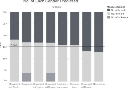
Figure 3. Number of each gender predicted.

Also, since the gender ratio generated is 1:1. Intuitively, model with prediction closer to this ratio tend to be less biased. According to Fig. 3, both unweighted and weighted clustering models bias the most among these four algorithms. Decision tree and logistic regression are close to this ratio the most. Therefore, decision tree and logistic regression are the unbiased model.

Conclusions and Future Work

While considering the natural gender orientation of smartphone applications, the impact of prevalence and balance between applications, our weighted average model still has the advantage of simple characteristic features compared to other high dimensional models. The evaluation indexes mentioned above are also valuable information for persona analysis.

The technique of weighted average feature really improves learning algorithms since all learning algorithms with weighted average features performance better than algorithms that are not: they have higher accuracy, lower MSE and more balanced proportion between male and female users. Though the difference of accuracy looks subtle, when the sample size is large, the absolute difference of number of correct prediction can be huge. Same comparison process repeated again for real dataset, and it shows the same conclusion as our simulated data.

Both weighted logistic regression model and decision tree have stable predictions. They have relatively high accuracy and unbiased prediction between female and male. Therefore, we propose these two weighted average featured models as the most efficient learning algorithms to predict users gender based on their mobile applications installed.

Reference

[1] Seneviratne S, Seneviratne A, Mohapatra P, et al. Predicting user traits from a snapshot of apps installed on a smartphone[J]. ACM Sigmobile Mobile Computing & Communications Review, 2014, 18(2):1-8.

[2] Malmi E, Weber I. You Are What Apps You Use: Demographic Prediction Based on User's Apps[J]. 2016.

[3] D. Kelly, S. Brendan, and C. Brian, “Uncovering Measurements of Social and Demographic Behavior from Smartphone Location Data,” IEEE Transactions on Human-Machine Systems, vol. 43, no. 2, pp. 188–198, 2013.

[4] Mislove, A.; Lehmann, S.; Ahn, Y.-Y.; Onnela, J.-P.; and Rosenquist, J. N. 2011. Understanding the demographics of twitter users. In Proc. ICWSM.

[5] JJ Ying, Y Chang, C Huang, VS Tseng. Demographic prediction Based on User’s Mobile Behaviors[C]. Nokia Mobile Data Challenge 2012 Workshop. Newcastle, UK. 2012.

M odels

Unw eight ed Clust ..

Diagnoal Unw eight ed Logis..

Unw eight ed Diagn..

Logist ic r egr ession

Decision t r ee

Unw eight ed Decisi..

Clust er ing 0K

5K 10K 15K 20K 25K 30K

V

a

lu

e

15,000

No. of Each Gender Pr edict ed

Measur e Names

[6] Wang Y, Tang Y, Ma J, et al. Gender Prediction Based on Data Streams of Smartphone Applications[M]// Big Data Computing and Communications. Springer International Publishing, 2015.

[7] Yong Xia. User’s Demographic Prediction Based on Smartphone Application Logs.[D]. University of Electronic Science and Technology of China, 2015.

[8] Qin Z, Wang Y, Cheng H, et al. Demographic Information Prediction: A Portrait of Smartphone Application Users[J]. IEEE Transactions on Emerging Topics in Computing, 2016, PP(99):1-1.

[9] Information on http://www.questmobile.com.cn/blog/blog_80.html.

[10] Pfitzner, Darius; Leibbrandt, Richard; Powers, David (2009). "Characterization and evaluation of similarity measures for pairs of clusterings". Knowledge and Information Systems. Springer. 19: 361–394. doi:10.1007/s10115-008-0150-6

[11] Peter J. Rousseeuw (1987). "Silhouettes: a Graphical Aid to the Interpretation and Validation of Cluster Analysis". Computational and Applied Mathematics. 20: 53–65. doi:10.1016/0377-0427(87)90125-7