The London School of Economics and Political Science
OPTIMAL STOPPING PROBLEMS
IN MATHEMATICAL FINANCE
by
Neofytos Rodosthenous
A thesis submitted to the Department of Mathematics of the London School of Economics and Political Science
for the degree of Doctor of Philosophy
London, May 2013
Declaration
I certify that the thesis I have presented for examination for the MPhil/PhD degree of the London School of Economics and Political Science is solely my own work other than where I have clearly indicated that it is the work of others (in which case the extent of any work carried out jointly by me and any other person is clearly identified in it).
The copyright of this thesis rests with the author. Quotation from it is permitted, provided that full acknowledgement is made. This thesis may not be reproduced without my prior written consent.
I warrant that this authorisation does not, to the best of my belief, infringe the rights of any third party.
Abstract
This thesis is concerned with the pricing of American-type contingent claims.
First, the explicit solutions to the perpetual American compound option pricing problems in the Black-Merton-Scholes model for financial markets are presented. Compound options are financial contracts which give their holders the right (but not the obligation) to buy or sell some other options at certain times in the future by the strike prices given. The method of proof is based on the reduction of the initial two-step optimal stopping problems for the underlying geometric Brownian motion to appropriate sequences of ordinary one-step problems. The lat-ter are solved through their associated one-sided free-boundary problems and the subsequent martingale verification for ordinary differential operators. The closed form solution to the per-petual American chooser option pricing problem is also obtained, by means of the analysis of the equivalent two-sided free-boundary problem.
Second, an extension of the Black-Merton-Scholes model with piecewise-constant dividend and volatility rates is considered. The optimal stopping problems related to the pricing of the perpetual American standard put and call options are solved in closed form. The method of proof is based on the reduction of the initial optimal stopping problems to the associated free-boundary problems and the subsequent martingale verification using a local time-space formula. As a result, the explicit algorithms determining the constant hitting thresholds for the underlying asset price process, which provide the optimal exercise boundaries for the options, are presented.
Third, the optimal stopping games associated with perpetual convertible bonds in an ex-tension of the Black-Merton-Scholes model with random dividends under different information flows are studied. In this type of contracts, the writers have a right to withdraw the bonds before the holders can exercise them, by converting the bonds into assets. The value functions and the stopping boundaries’ expressions are derived in closed-form in the case of observable dividend rate policy, which is modelled by a continuous-time Markov chain. The analysis of the associated parabolic-type free-boundary problem, in the case of unobservable dividend rate policy, is also presented and the optimal exercise times are proved to be the first times at which the asset price process hits boundaries depending on the running state of the filtering dividend rate estimate. Moreover, the explicit estimates for the value function and the optimal exercise boundaries, in the case in which the dividend rate is observable by the writers but unobservable by the holders of the bonds, are presented.
Contents
Introduction . . . 5
I. Description of the subject . . . 5
II. Historical notes and references . . . 6
III. Contribution of the thesis . . . 11
IV. Summary of the thesis . . . 13
V. Acknowledgements . . . 14
1. On the pricing of perpetual American compound options . . . 16
1.1. Preliminaries . . . 16
1.2. Solutions of the free-boundary problems . . . 20
1.3. Main results and proofs . . . 25
1.4. Chooser options . . . 29
2. Perpetual American options in a diffusion model with piecewise-linear coefficients . . . 36
2.1. Preliminaries . . . 36
2.2. Solutions of the free-boundary problem . . . 38
2.3. Main results and proof . . . 49
3. Optimal stopping games in models with different information flows . . . 53
3.1. Preliminaries . . . 53
3.2. The case of full information . . . 59
3.3. The case of partial information . . . 74
3.4. The case of asymmetric information . . . 80
4. Optimal stopping problems in diffusion-type models with running maxima and drawdowns . . . 82
4.1. Preliminaries . . . 82
4.2. Solution of the free-boundary problem . . . 86
4.3. Main results and proof . . . 97
Introduction
I. Description of the subject
The focus of this thesis is optimal stopping problems, which is an important and well-developed class of stochastic control problems. In such problems, we aim to find stopping times, at which the underlying stochastic processes should be stopped in order to optimise the values of some given functionals (e.g. maximise gain functions, minimise loss functions, etc). These kind of problems appear in various different research areas in sciences, one of which is
mathematical finance. A great deal of thederivativestraded in the financial markets all over the world is of the so-calledAmerican-type. Contrary to the European-type derivatives, the holders of which have the opportunity to exercise only at a fixed maturity time, the American-type derivatives can be exercised at any time up to maturity. The rational (no-arbitrage) prices of such contracts are given by the values of their associated optimal stopping problems, which are considered under some martingale measures for the underlying risky asset price processes. A broad overview of the general theory, explanations of the main concepts and results, examples and proofs of key facts as well as the principles of the methods used for solving optimal stopping problems in various stochastic models can be found in [97], [105; Chapter VIII], [70] and [44].
A formulation of the general optimal stopping problem for sequences of random variables and the establishment of the supermartingale characterization of its value function was presented by Snell [107]. Then, it was observed by Dynkin [31] that the proposed in [107] supermartin-gale characterization of the value function of an optimal stopping problem is superharmonic, whenever the underlying sequence of random variables is Markovian. This resulted to further development of the field by allowing for more concrete results.
given functionals in continuous Markov models can be obtain in analytic expressions. The closed-form solutions of these free-boundary problems satisfying certain additional conditions
are then proved to be the solutions of the initial optimal stopping problems, through some standard verification arguments from stochastic analysis. These include the application of the relevant change-of-variable formula (i.e. Itˆo’s formula or its various extensions) and Doob’s op-tional sampling theorem. A complete overview of the optimal stopping theory for both discrete-and continuous-time Markov processes can be found in the monograph of Shiryaev [104].
In order to select the unique solution of the free-boundary problem, which will eventually turn out to be the solution of the initial optimal stopping problem, the specification of these
additional conditions in the free-boundary problems becomes essential. It was observed and then proved by many different authors, that if the underlying process exits the continuation region continuously, then the smooth-fit condition for the value function at the optimal stopping boundary should hold. Different proofs of the principle of smooth fit in continuous Markov models are contained in [104; Chapter III] and [97; Chapter IV]) (see also [58] for sufficient conditions for the occurrence of smooth fit in a general multi-dimensional continuous Markov model).
The value function, obtained as a solution of optimal stopping problems involving the running maximum process of continuous Markov (diffusion) processes, satisfies the normal-reflection condition on the diagonal of the state space of the two-dimensional process, whose components are given by the underlying and its running maximum. This fact was proved by Dubins, Shepp and Shiryaev [28] through the solution of the optimal stopping problem, which appeared in the proof of the related maximal inequalities for Bessel processes on random time intervals in stochastic calculus. A key result in the general theory, which proved that the
maximality principle is equivalent to the superharmonic characterization of the value function, was established by Peskir [90], through the solution of the same problem in a general diffusion model (see also [64], [56]-[57]).
II. Historical notes and references
Let us now present some historical notes on the optimal stopping problems studied in this thesis and refer to the relevant literature, by also specifying the position of the results of this thesis.
common application of such contracts is the hedging of bids for business opportunities which may or may not be accepted in the future, and which become available only after the previous ones are undertaken. This fact makes compound options an important example of using real options to undertake business decisions which can be expressed in the presented perspective (see Dixit and Pindyck [27] for an extensive introduction). Other important modifications of such contracts are compound contingent claims ofAmerican type in which both the initial and underlying options can be exercised at any (random) times up to maturity. The rational (no-arbitrage) pricing problems for such contracts are considered in [48] (Chapter 1), where they are embedded into two-step optimal stopping problems for the underlying asset price processes. The latter are decomposed into appropriate sequences of ordinary one-step optimal stopping problems which are then solved sequentially.
Apart from the extensive literature on optimal switching as well as impulse and singular stochastic control, the multi-step optimal stopping problems for underlying one-dimensional diffusion processes have recently drawn a considerable attention. Duckworth and Zervos [29] studied an investment model with entry and exit decisions alongside a choice of the production rate for a single commodity. The initial valuation problem was reduced to a two-step optimal stopping problem which was solved through its associated dynamic programming differential equation. Carmona and Touzi [19] derived a constructive solution to the problem of pricing of perpetual swing contracts, the recall components of which could be viewed as contingent claims with multiple exercises of American type, using the connection between optimal stopping prob-lems and their associated Snell envelopes. Carmona and Dayanik [18] then obtained a closed form solution of a multi-step optimal stopping problem for a general linear regular diffusion pro-cess and a general payoff function. Algorithmic constructions of the related exercise boundaries were also proposed and illustrated with several examples of such optimal stopping problems for several linear and mean-reverting diffusions. Other infinite horizon optimal stopping problems with finite sequences of stopping times are being sought. Some of them are related to hiring and firing options and were recently considered by Egami and Xu [33] among others.
Alili and Kyprianou [4] proved the optimality of the threshold strategies for the underlying process and derived closed form expressions for the values of these optimal stopping problems in several exponential L´evy models. Some associated optimal stopping games for such processes were recently studied by Baurdoux and Kyprianou [9] among others.
The framework of the so-called local models of stochastic volatility, in which the diffusion coefficients depend on both the time and the current state of the underlying risky asset price process, was proposed by Dupire [30] and Derman and Kani [25]. Apart from easy calibration features (see, e.g. [30] and [25]), such extensions of the classical model with constant coeffi-cients remained within complete market setting in which any contingent claim can be replicated by an admissible self-financing portfolio strategy, based on the underlying asset and the risk-less bank account only. More recently, Ekstr¨om [34]-[35] found explicit values for the rational prices of the perpetual American options and investigated their properties in some diffusion models with time- and state-dependent volatility coefficients. The call-put duality for perpet-ual American options was studied by Alfonsi and Jourdain [2]-[3] within a local volatility and constant dividend yield framework. Villeneuve [109] proposed a model with both the volatil-ity and dividend yield coefficients depending on the underlying price process and investigated sufficient conditions on the payoff functions ensuring the optimality of the constant threshold exercise strategies for the perpetual American options. The closed-form solutions to the per-petual American put and call options in a diffusion model with piecewise-constant dividend and volatility coefficients are presented in [49] (Chapter 2). Using a geometric approach, Lu [80] presented a solution of the optimal stopping problem related to the perpetual American put option in a dividend-free model with piecewise-constant volatility rate. He also studied the inverse problem of recovering the volatility rate of such type from the perpetual put option prices, initiated by Ekstr¨om and Hobson [36] within the general local volatility framework.
Optimal stopping problems for general time-homogeneous one-dimensional diffusion pro-cesses were studied in Salminen [101] and Beibel and Lerche [13] for the cases of deterministic and random discounting, respectively. Dayanik and Karatzas [24] provided a characterization of the value functions of the optimal stopping problems for such general diffusions as the smallest nonnegative concave majorants of the reward functions. R¨uschendorf and Urusov [100] used the free-boundary approach to study optimal stopping problems for integral functionals of general one-dimensional diffusion processes, the coefficients of which do not satisfy the usual regularity assumptions. More recently, Christensen and Irle [21] characterized stopping regions of optimal stopping problems in terms of harmonic functions for general one-dimensional diffusions.
analysis of such games, based on the application of martingale theory, was developed in Neveu [85], Krylov [74], Bismut [17], Stettner [108], and Lepeltier and Mainguenau [78] among others. The analytical theory of stochastic differential games with stopping times was developed in Bensoussan and Friedman [14]-[15] in Markov diffusion models. The latter approach, dealing with the analysis of the value functions and saddle points of such games, was based on the usage of the theory of variational inequalities and free-boundary problems for partial differential equations. Cvitanic and Karatzas [22] established a connection between the values of optimal stopping games and the solutions of backward stochastic differential equations with reflection and provided a pathwise approach to these games. Karatzas and Wang [71] studied such games in a more general non-Markovian setting and brought them into connection with bounded-variation optimal control problems. More recently, Ekstr¨om and Peskir [37] and Peskir [93]-[95] proved that the value function of a general optimal stopping game for a right-continuous strong Markov process is measurable and found necessary and sufficient conditions for the existence of the Stackelberg and Nash equilibria. Bayraktar and Sirbu [12] applied stochastic Perron’s method and verification without smoothness using viscosity comparison for solving obstacle problems and Dynkin games.
The related concept of the so-called game-type (or Israeli) contingent claims for models of financial markets was introduced by Kifer [73], who generalised the one of American-type claims, by also allowing the writer to cancel the contract prematurely at the expense of some penalty. It was shown that the problem of pricing and hedging of such options can be reduced to solving an associated optimal stopping game. Kyprianou [77] obtained explicit expressions for the value functions of two classes of perpetual game option problems. K¨uhn and Kyprianou [76] characterized the value functions of the finite expiry versions of these classes of options via mixtures of other exotic options using martingale arguments and then produced the same analysis for a more general class of finite expiry game options via a pathwise pricing formulae. Kallsen and K¨uhn [67]-[68] applied the neutral valuation approach to American and game options in incomplete markets and introduced a mathematically rigorous dynamic concept to define no-arbitrage prices for game contingent claims. Sirbu, Pikovsky and Shreve [106] studied the convertible bond optimal stopping game within a structural model for the underlying risky asset. Further calculations of rational prices of perpetual game options and convertible bonds in reduced form models involving jump-diffusion structure were provided by Baurdoux and Kyprianou [8]-[10], Ekstr¨om and Villeneuve [38], and Baurdoux, Kyprianou and Pardo [11] among others, and involving random-dividend structure, modelled by a continuous Markov chain (under different information flows), are provided in Chapter 3.
perpetual American lookback and put option pricing problems were obtained by Guo [59] and Guo and Zhang [62] in a version of such a model in which the drift and volatility coefficients of the underlying asset price process are switching between two constant values, according to the change in the state of the observable continuous-time Markov chain. Jobert and Rogers [66] considered the perpetual American put option problem within an extension of that model to the case of several states for the Markov chain and solved the corresponding problem with finite expiry numerically. In the model with a two-state Markov chain and no diffusion part, Dalang and Hongler [23] presented a complete and essentially explicit solution to a similar problem, which exhibited a surprisingly rich structure. These results were further extended by Jiang and Pistorius [65], who studied the perpetual American put option problem within the framework of an exponential jump-diffusion model with observable dynamics of regime-switching behaving parameters.
Optimal stopping problems forrunning maximaof some diffusion processes given linear costs were studied by Jacka [64], Dubins, Shepp, and Shiryaev [28], and Graversen and Peskir [56]-[57] among others, with the aim of determining the best constants in the corresponding maximal inequalities. A complete solution of a general version of the same problem was obtained in Peskir [90], by means of the established maximality principle which is equivalent to the superharmonic characterization of the value function. Discounted optimal stopping problems for certain payoff functions depending on the running maxima of geometric Brownian motions were initiated by Shepp and Shiryaev [102]-[103] and then considered by Pedersen [89] and Guo and Shepp [60] among others, with the aim of computing rational values of perpetual American lookback (Russian) options. More recently, Guo and Zervos [61] derived solutions for discounted optimal stopping problems related to the pricing of perpetual American options with certain payoff functions depending on the running values of both the initial diffusion process and its associated maximum. Glover, Hulley, and Peskir [55] provided solutions of optimal stopping problems for integrals of functions depending on the running values of both the initial diffusion process and its associated minimum. The main feature of the resulting optimal stopping problems is that the normal-reflection condition holds for the value function at the diagonal of the state space of the two-dimensional continuous Markov process having the initial process and its running extremum as the components, which implies the characterization of the optimal boundaries as extremal solutions of one-dimensional first-order nonlinear ordinary differential equations.
considered by Baurdoux and Kyprianou [10] within the framework of models based on spec-trally negative L´evy processes. Other complicated optimal stopping problems for the running maxima were considered by Gapeev [43] for a jump-diffusion model with compound Poisson processes with exponentially distributed jumps and by Ott [87] (see also [88]) for a model based on spectrally negative L´evy processes. More recently, Peskir [94]-[96] studied optimal stopping problems for three-dimensional Markov processes having the initial diffusion process as well as its maximum and minimum as the state space components. It was shown that the optimal boundary surfaces depending on the maximum and minimum of the initial process provide the maximal and minimal solutions of the associated systems of first-order non-linear partial differential equations. The perpetual American strangle options pricing problems in a diffusion-type extension of the Black-Merton-Scholes model, for which the dividend and the volatility coefficients depend on both the running maximum and maximum drawdown processes of the underlying, are studied in Chapter 4. The drawdown process represents the difference between the running values of the underlying asset price and its maximum and can therefore be interpreted as the market depth. The Laplace transforms of the drawdown process and other related characteristics associated with certain classes of the initial processes such as diffusion models (including constantly drifted Brownian motions, the Ornstein-Uhlenbeck process and the Cox-Ingersoll-Ross model), and spectrally positive and negative L´evy processes were studied by Pospisil, Vecer, and Hadjiliadis [98] and by Mijatovic and Pistorius [82], respectively.
III. Contribution of the thesis
Let us now summarise the contribution of the thesis into the methods of optimal stopping problems and their applications.
framework. The associated two-step free-boundary problems for partial differential equations were solved numerically, by means of a modified sparse grid approach.
The rational prices of the perpetual American standard put and call options in an extension of the Black-Merton-Scholes model for underlying dividend paying assets with both piecewise-constant dividend and volatility rates are presented (Chapter 2 or [49]). It is assumed that these rates change their values at the times at which the underlying asset price process crosses some prescribed constant levels under the risk-neutral probability measure. Such a situation may appear in the case in which either the firm issuing the asset decides to change the dividend rate paid to stockholders or the volatility rate of the asset changes from one value to another at the times at which the market price crosses certain levels. These levels can have both statistical and psychological nature depending on the strategies of market participants. This model represents another example of local models of stochastic dividend and volatility, in which the related coefficients depend on the current state of the underlying asset price process and provides an approximation of the corresponding diffusion models with continuous coefficients studied in [34]-[35], [2]-[3], and [109]. A linear version of this diffusion model was proposed by Radner and Shepp [99] with the aim of solving some stochastic optimal impulse control problems. Explicit algorithms to determine the constant hitting thresholds for the underlying diffusion process, which provide the optimal exercise boundaries for the options, are presented. Based on solving the associated free-boundary problems, our approach should allow to handle optimal stopping problems with more complicated payoffs than the ones of put and call options, within the general diffusion framework of both piecewise-linear drift and diffusion coefficients. The perpetual convertible bond pricing problem is studied in an extension of the Black-Merton-Scholes model in which the dynamics of the dividend rate of the underlying risky asset are described by means of a two-state continuous-time Markov chain (Chapter 3). Closed-form solutions to the associated optimal stopping games for the case in which the Markov chain is observable by both the writer and the holder of the convertible bond (full information) are de-rived. An analysis of the equivalent parabolic-type free-boundary problem for the case in which the Markov chain is unobservable by both participants of the contract (partial information) is also presented, as well as the case in which the Markov chain is observable by the writer but remains unobservable by the holder of the bond (asymmetric information) is studied.
values of S and Y. The process Y represents the maximum of the difference between the running values of the underlying asset price and its maximum and can therefore be interpreted as the maximum of the market depth. Closed-form expressions for the value function of the resulting free-boundary problem are derived and the maximality principle from [90] is applied to describe the optimal boundary surfaces as the extremal solutions of first-order nonlinear ordinary differential equations. The starting points for these surfaces at the edges of the three-dimensional state space are specified from the solutions of the corresponding optimal stopping problem for the two-dimensional Markov process (X, S) in a model in which the coefficients of the process X depend only on the running maximum process S.
IV. Structure of the thesis
In Section 1.1, we formulate the perpetual American compound option problems and then specify the decompositions of the initial two-step optimal stopping problems into sequences of ordinary one-step problems for the underlying geometric Brownian motion. In Section 1.2, we derive explicit solutions of the four resulting one-sided ordinary differential free-boundary problems. In Section 1.3, we verify that the solution of the free-boundary problem related to the most informative put-on-call case provides the solution of the initial two-step optimal stopping problem. In Section 1.4, we present a closed form solution to the two-sided free-boundary problem associated with the perpetual American chooser option. The main results of Chapter 1 are stated in Propositions 1.3.1-1.3.4 and 1.4.1.
In Section 2.1, we formulate the perpetual American put and call option pricing optimal stopping problems in a diffusion model with piecewise-linear coefficients and their associated ordinary differential free-boundary problems. In Section 2.2, we derive solutions to the resulting systems of arithmetic equations equivalent to the free-boundary problems for the put and call options, separately. In Section 2.3, we verify that the solutions of the free-boundary problems provide the solutions of the initial optimal stopping problems. The main result of Chapter 2 is stated in Theorem 2.3.1.
problem equivalent to the optimal stopping game in the case of an unobservable Markov chain. Applying the change-of-variable formula with local time on surfaces from Peskir [92], we verify that the appropriate (unique) solution of the free-boundary problem gives the solution to the initial optimal stopping game. We also obtain a closed-form solution of the free-boundary prob-lem under certain relations between the parameters of the model. In Section 3.4, we propose a solution to the optimal stopping game for the case in which the Markov chain is observable by the writer but remains unobservable by the holder of the bond. The main results of Chapter 3 are stated in Theorems 3.2.1 and 3.3.1, and Corollary 3.4.1.
In Section 4.1, we formulate the associated optimal stopping problem for a necessarily three-dimensional continuous Markov process which has the underlying asset price and the running values of its maximum and maximum drawdown as the state space components. The resulting optimal stopping problem is reduced to its equivalent free-boundary problem for the value function which satisfies the smooth-fit conditions at the stopping boundaries and the normal-reflection conditions at the edges of the state space of the three-dimensional process. In Section 4.2, we obtain closed-form solutions of the associated free-boundary problem in which the sought boundaries are found as unique solutions of appropriate systems of arithmetic equations or first-order nonlinear ordinary differential equations, where we specify the starting values for the latter on the edges of the three-dimensional state space. In Section 4.3, we verify by applying the change-of-variable formula with local time on surfaces, that the resulting solutions of the free-boundary problem provide the expressions for the value function and the optimal stopping boundaries for the underlying asset price process in the initial problem. The main results of Chapter 4 are stated in Propositions 4.3.1-4.3.3.
V. Acknowledgements
I would like to express my gratitude and appreciation to Mihail Zervos and Pavel V. Gapeev for the endless hours they invested, not only to enhance my mathematical knowledge, particu-larly in stochastic control theory, but also to help me develop my own way of thinking. I am grateful they played such an important role in the fulfillment of this thesis and for setting the example of an intellectual, which has been most influential.
I gratefully acknowledge the support from the Alexander Onassis Public Benefit Foundation in Greece and their contribution to the realisation of this thesis by awarding me the scholarship for my doctoral studies.
as a fellow PhD student, my friend Filippo Riccardi, with whom we studied for countless hours trying to understand several aspects of stochastic calculus.
During my studies, I have been fortunate to meet Ioannis Karatzas and Jean-Pierre Zigrand and I cannot thank them enough for showing me what it is like to be a truly inspirational and impactful teacher. I would also like to thank all the influential teachers I have had previously in my life, who contributed in the formation of my scientific thought. Especially, Haralambos Papageorgiou, whose continuous support and guidance has been vital.
I thank Hongzhong Zhang for his hospitality during my stay at the Columbia University and together with Olympia Hadjiliadis for our many fruitful discussions.
Chapter 1
On the pricing of perpetual American
compound options
In this chapter (following [48]), we present explicit solutions to the perpetual American com-pound option pricing problems in the Black-Merton-Scholes model. The method of proof is based on the reduction of the initial two-step optimal stopping problems for the underlying ge-ometric Brownian motion to appropriate sequences of ordinary one-step problems. The latter are solved through their associated one-sided free-boundary problems and the subsequent mar-tingale verification. We also obtain a closed form solution to the perpetual American chooser option pricing problem, by means of the analysis of the equivalent two-sided free-boundary problem.
1.1. Preliminaries
In this section, we give a formulation of the perpetual American compound option optimal stopping problems and the associated ordinary differential free-boundary problems.
1.1.1. Formulation of the problem. For a precise formulation of the problem, let us consider a probability space (Ω,F, P) carrying a standard one-dimensional Brownian motion B = (Bt)t≥0. Let us define the process S = (St)t≥0 by
St=s exp
r−δ−σ
2 2
t+σ Bt
(1.1.1)
which solves the stochastic differential equation
dSt= (r−δ)Stdt+σ StdBt (1.1.2)
We further consider the problem of pricing of the initial perpetual American standard
compound options, which are contracts giving their holders the right to buy or sell some other
underlying (perpetual American) call or put options at certain (random) exercise times by the (positive) strike prices given. More precisely, the call-on-call (call-on-put) option gives its holder the right to buy at an exercise time τ for the price of K1 a call (put) option with the strike K2 (L2) and exercise time ζ. Furthermore, the put-on-call (put-on-put) option gives its holder the right to sell at an exercise time τ for the price of L1 a call (put) option with the strike K2 (L2) and exercise time ζ. Then, the rational (or no-arbitrage) prices of such perpetual American contingent claims are given by the values of the optimal stopping problems
V1∗(s) = sup τ
sup ζ
Ehe−rτ e−r(ζ−τ)(Sζ−K2)+−K1
+i
(1.1.3)
V2∗(s) = sup τ
sup ζ
Ehe−rτ e−r(ζ−τ)(L2−Sζ)+−K1
+i
(1.1.4)
V3∗(s) = sup τ
inf ζ E
h
e−rτ L1−e−r(ζ−τ)(Sζ−K2)+
+i
(1.1.5)
V4∗(s) = sup τ
inf ζ E
h
e−rτ L1−e−r(ζ−τ)(L2−Sζ)+
+i
(1.1.6)
where the suprema and infima are taken over the sets of stopping times 0 ≤τ ≤ζ with respect to the natural filtration (Ft)t≥0 of the asset price process S, that is Ft=σ(Su |0≤u≤t), for all t ≥0. Here, the expectations are taken with respect to the equivalent martingale measure under which the dynamics of S started at s >0 are given by (1.1.1)-(1.1.2), and z+ denotes the positive part max{z,0} of any z∈R. Note that the payoff of the call-on-call option in (1.1.3) is unbounded, while the payoffs, and thus the related rational prices of the other options in (1.1.4)-(1.1.6), are bounded by L2 and L1, respectively. Moreover, it is easily seen from (1.1.4) and will be shown for (1.1.6) below that the optimal exercise times of the related options are trivial whenever K1 ≥L2 and L1 ≥L2 holds, respectively.
Observe that the value functions in (1.1.3)-(1.1.4) are given by the optimal sequential choices of τ and ζ, that results in the suprema over both such stopping times, since the holders of the initial compound options can buy the underlying calls or puts at the time τ and then control the exercise time ζ. This is not the case for the value functions in (1.1.5)-(1.1.6), due to the fact that, in the case in which the holders of the compound options exercise the initial puts at the time τ by selling the underlying calls or puts, they cannot control the subsequent exercise time ζ of the latter options. We should then assume that the holders of the underlying options exercise them optimally. This turns out to be the worst case scenario for the holders of the initial compound options, resulting in the infima over ζ in the expressions of (1.1.5)-(1.1.6).
one-step optimal stopping problems which can then be solved separately. More precisely, using the strong Markov property of the process S, we further show that the expressions for Vi∗(s), i= 1, . . . ,4, in (1.1.3)-(1.1.6) can be reduced to the values of the optimal stopping problems
Vi∗(s) = sup τ
Ee−rτHi+(Sτ)
(1.1.7)
where the payoff functions Hi(s), i= 1, . . . ,4, are given by
H1(s) =W(s)−K1, H2(s) = U(s)−K1, H3(s) = L1−W(s), H4(s) = L1−U(s) (1.1.8)
for all s >0. Here we denote the rational prices of the underlying perpetual American put and call options by U(s) and W(s) with strike prices L2 and K2, respectively. These are given by
U(s) = sup η
Ee−rη(L2−Sη)+
and W(s) = sup η
Ee−rη(Sη −K2)+
(1.1.9)
where the suprema are taken over the stopping times η of the process S started at s > 0. It is well known (see, e.g. [105; Chapter VIII, Section 2a]) that the value functions in (1.1.9) are continuously differentiable and have the form
U(s) =
−(g∗/γ−)(s/g∗)γ−, if s > g∗
L2−s, if s≤g∗
(1.1.10)
and
W(s) =
(h∗/γ+)(s/h∗)γ+, if s < h∗ s−K2, if s≥h∗.
(1.1.11)
The optimal exercise times have the structure
ηg∗ = inf{t ≥0|St ≤g∗} and ηh∗ = inf{t≥0|St≥h∗} (1.1.12)
and the hitting boundaries are given by
g∗ = γ−L2 γ−−1
and h∗ =
γ+K2 γ+−1
(1.1.13)
with
γ± = 1 2 −
r−δ σ2 ±
s
1 2 −
r−δ σ2
2
+ 2r
σ2 (1.1.14)
so that γ− <0<1< γ+ holds.
It follows from the general theory of optimal stopping for Markov processes (see, e.g. [97; Chapter I, Section 2.2]) that the optimal stopping times in the problems of (1.1.7)-(1.1.8) are given by
whenever they exist. Analysing the structure of the outer and inner payoffs in (1.1.3)-(1.1.6), we observe that the call-on-call and put-on-put options should be exercised at the first time at which the price of the underlying risky asset rises to some upper levels b∗i, while the call-on-put and call-on-put-on-call options should be exercised at the first time at which the asset price falls to some lower levels a∗i. Hence, we need further to search for optimal stopping times in the problems of (1.1.7)-(1.1.8) in the form
τi∗ = inf{t≥0|St≤a∗i} or τ ∗
i = inf{t ≥0|St ≥b∗i} (1.1.16)
for some a∗i >0 and b∗i >0 to be determined, where the left-hand stopping time in (1.1.16) is optimal for the cases of i = 2,3, and the right-hand one is optimal for the cases of i = 1,4. Taking into account the structure of the stopping times in (1.1.12), we then further assume that the optimal stopping times ζi∗ in (1.1.3)-(1.1.6) have the form
ζi∗ = inf{t≥τi∗ |St≤g∗} or ζi∗ = inf{t≥τi∗ |St≥h∗} (1.1.17)
depending on the view of the payoff functions of the underlying options.
1.1.3. The free-boundary problem. It can be shown by means of standard arguments (see, e.g. [69; Chapter V, Section 5.1] or [86; Chapter VII, Section 7.3]) that the infinitesimal operator L of the process S acts on an arbitrary twice continuously differentiable locally bounded function F(s) according to the rule
(LF)(s) = (r−δ)s F0(s) + σ 2 2 s
2F00
(s) (1.1.18)
for all s > 0. In order to find explicit expressions for the unknown value functions Vi∗(s), i= 1, . . . ,4, from (1.1.7)-(1.1.8) and the unknown boundaries a∗i and b∗i from (1.1.16), we may use the results of the general theory of optimal stopping problems for continuous time Markov processes (see, e.g. [104; Chapter III, Section 8] and [97; Chapter IV, Section 8]). We formulate the associated free-boundary problems
(LVi)(s) =rVi(s) for s > ai or s < bi (1.1.19) Vi(ai+) =Hi+(ai) or Vi(bi−) = Hi+(bi) (instantaneous stopping) (1.1.20) Vi0(ai+) =Hi+
0
(ai) or Vi0(bi−) = Hi+ 0
(bi) (smooth fit) (1.1.21)
1.2. Solutions of the free-boundary problems
We further derive solutions of the free-boundary problems related to the optimal stopping problems in (1.1.7)-(1.1.8), by specifying whether the left-hand or the right-hand part of the system in (1.1.19)-(1.1.24) is realised in every case of i = 1, . . . ,4. For this we first note that the general solution of the second order ordinary differential equation in (1.1.19) is given by
Vi(s) =C+,isγ+ +C
−,isγ− (1.2.1)
where C+,i and C−,i are some arbitrary constants, andγ−<0<1< γ+ are defined in (1.1.14). Observe that we should have C−,i = 0 in (1.2.1) when the right-hand part of the system in (1.1.19)-(1.1.24) is realised, since otherwise Vi(s)→ ±∞, which must be excluded because the value functions in (1.1.7) are bounded under s ↓ 0. Similarly, we should also have C+,i = 0 in (1.2.1) when the left-hand part of the system in (1.1.19)-(1.1.24) is realised, since otherwise Vi(s) → ±∞, which must be excluded because the value functions in (1.1.7) are less than s under s ↑ ∞.
1.2.1. The call-on-call option. Let us first consider the case of i= 1 in which the right-hand stopping time from (1.1.16) is optimal in (1.1.3) and (1.1.7)-(1.1.8), so that the right-right-hand part of the free-boundary problem is realised in (1.1.19)-(1.1.24). Applying the conditions of the right-hand parts of the equations in (1.1.20) and (1.1.21) to the function in (1.2.1) with C−,1 = 0, we obtain after some rearrangements that if b1 < h∗ then the equalities
C+,1bγ+
1 = h∗ γ+
b1
h∗
γ+
−K1 and C+,1γ+bγ+
1 =h∗
b1
h∗
γ+
(1.2.2)
should hold, and if b1 ≥h∗ then the equalities
C+,1bγ+
1 =b1−K2 −K1 and C+,1γ+b γ+
1 =b1 (1.2.3)
are satisfied for some C+,1 and b1 > 0, where h∗ is given by (1.1.13). Multiplying the first equation in (1.2.2) by γ+, we conclude from the second one there that the system in (1.1.19)-(1.1.21) does not have solutions, so that the subcase b∗1 < h∗ cannot be realised. Solving the system in (1.2.3), we obtain the solution of the right-hand part of the system in (1.1.19)-(1.1.21) having the form
V1(s;b∗1) = b∗1 γ+
s
b∗ 1
γ+
with b∗1 = γ+(K1+K2) γ+−1
≡ γ+K1
γ+−1
+h∗. (1.2.4)
of the left-hand parts of the equations in (1.1.20) and (1.1.21) to the function in (1.2.1) with C+,2 = 0, we obtain after some rearrangements that if a2 > g∗ then the equalities
C−,2aγ2− =− g∗ γ−
a2
g∗
γ−
−K1 and C−,2γ−aγ2− =−g∗
a2
g∗
γ−
(1.2.5)
should hold, and if a2 ≤g∗ then the equalities
C−,2aγ2− =L2−a2−K1 and C−,2γ−aγ2− =−a2 (1.2.6)
are satisfied for some C−,2 and a2 > 0, where g∗ is given by (1.1.13). Multiplying the first equation in (1.2.5) by γ−, we conclude from the second one there that the system in (1.1.19)-(1.1.21) does not have solutions, so that the subcase a∗2 > g∗ cannot be realised. Solving the system in (1.2.6), we obtain the solution of the left-hand part of the system in (1.1.19)-(1.1.21) having the form
V2(s;a∗2) =− a∗2 γ−
s
a∗ 2
γ−
with a∗2 = γ−(L2−K1) γ−−1
≡g∗−
γ−K1 γ−−1
(1.2.7)
where the number a∗2 is strictly positive if and only if L2 > K1.
-6
h∗ b∗1
@
@
@
@ @ R
V1∗(s)
X X X X X X y
H1(s) V
[image:22.612.120.483.308.716.2]s
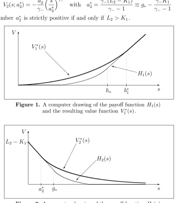
Figure 1. A computer drawing of the payoff function H1(s)
and the resulting value function V1∗(s) .
-6
a∗2 g∗ L2−K1
V2∗(s)
H2(s) V
[image:22.612.124.471.558.715.2]s
Figure 2. A computer drawing of the payoff function H2(s)
1.2.3. The put-on-call option. Let us now continue with the case of i= 3 in which the hand stopping time from (1.1.16) is optimal in (1.1.5) and (1.1.7)-(1.1.8), so that the left-hand part of the free-boundary problem is realised in (1.1.19)-(1.1.24). Applying the conditions of the left-hand parts of the equations in (1.1.20) and (1.1.21) to the function in (1.2.1) with C+,3 = 0, we get after some rearrangements that if a3 < h∗ then the equalities
C−,3a γ−
3 =L1− h∗ γ+
a3
h∗
γ+
and C−,3γ−aγ3− =−h∗
a3
h∗
γ+
(1.2.8)
hold, and if a3 ≥h∗ then the equalities
C−,3a γ−
3 =L1−a3+K2 and C−,3γ−aγ3− =−a3 (1.2.9) are satisfied for some C−,3 and a3 >0, where h∗ is given by (1.1.13). Solving the systems in (1.2.8) and (1.2.9), we conclude that the two regions for L1 and K2, with qualitatively different solutions of the free-boundary problem, can be distinguished. By means of straightforward computations, if the condition
L1 <
γ−−γ+ γ+γ−
h∗ ≡
(γ−−γ+)K2 γ−(γ+−1)
(1.2.10)
is satisfied, then a∗3 < h∗ holds and the solution of the left-hand part of the system in (1.1.19)-(1.1.21) has the form
V3(s;a∗3, h∗) = − h∗ γ−
a∗
3 h∗
γ+s
a∗3
γ−
(1.2.11)
with
a∗3 =h∗
γ+γ−L1
(γ−−γ+)h∗
1/γ+
≡ γ+K2
γ+−1
γ−(γ+−1)L1
(γ−−γ+)K2
1/γ+
. (1.2.12)
Using similar arguments, if the condition
L1 ≥
γ−−γ+ γ+γ−
h∗ ≡
(γ−−γ+)K2 γ−(γ+−1)
(1.2.13)
is satisfied, then a∗3 ≥h∗ holds and the solution of the left-hand part of the system in (1.1.19)-(1.1.21) has the form
V3(s;a∗3) =−a
∗ 3 γ−
s
a∗3
γ−
with a∗3 = γ−(L1+K2) γ−−1
. (1.2.14)
1.2.4. The put-on-put option. Let us finally consider the case of i = 4 in which the right-hand stopping time from (1.1.16) is optimal in (1.1.6) and (1.1.7)-(1.1.8), so that the right-hand part of the free-boundary problem is realised in (1.1.19)-(1.1.24). Applying the conditions of the right-hand parts of the equations in (1.1.20) and (1.1.21) to the function in (1.2.1) with C−,4 = 0, we get after some rearrangements that if b4 > g∗ then the equalities
C+,4bγ4+ =L1+ g∗ γ−
b4
g∗
γ−
and C+,4γ+bγ4+ =g∗
b4
g∗
γ−
hold, and if b4 ≤g∗ then the equalities
C+,4b γ+
4 =L1−L2+b4 and C+,4γ+b γ+
4 =b4 (1.2.16)
are satisfied for some C+,4 and b4 >0. Solving the systems in (1.2.15) and (1.2.16), we conclude that the two regions for L1 and L2, with qualitatively different solutions of the free-boundary problem (besides the trivial solution in the case L1 ≥ L2), can be distinguished. By means of straightforward computations, if the condition
L1 <
γ−−γ+ γ+γ−
g∗ ≡
(γ−−γ+)L2 γ+(γ−−1)
(1.2.17)
is satisfied, then b∗4 > g∗ holds and the solution of the left-hand part of the system in (1.1.19)-(1.1.21) has the form
V4(s;b∗4, g∗) = g∗ γ+
b∗
4 g∗
γ−s
b∗4
γ+
(1.2.18)
with
b∗4 =g∗
γ+γ−L1
(γ−−γ+)g∗
1/γ−
≡ γ−L2
γ−−1
γ+(γ−−1)L1
(γ−−γ+)L2
1/γ−
. (1.2.19)
Using similar arguments, if the condition
L1 ≥
γ−−γ+ γ+γ−
g∗ ≡
(γ−−γ+)L2 γ+(γ−−1)
(1.2.20)
is satisfied, then b∗4 ≤g∗ holds and the solution of the left-hand part of the system in (1.1.19)-(1.1.21) has the form
V4(s;b∗4) = b ∗ 4 γ+
s
b∗4
γ+
with b∗4 = γ+(L2−L1) γ+−1
(1.2.21)
where the number b∗4 is strictly positive if and only if L2 > L1.
-6
a∗3 h∗
L1
XX XX
XX XXz
H3(s)
V3∗(s) V
[image:24.612.128.470.556.708.2]s
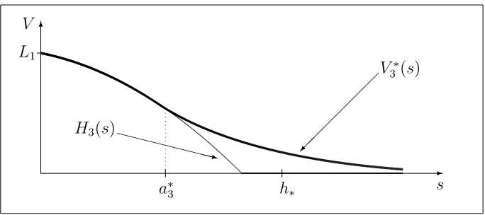
Figure 3. A computer drawing of the payoff function H3(s) and
-6
h∗ a∗3 L1
XX XX
XX XXz
H3(s)
V3∗(s) V
[image:25.612.127.471.102.255.2]s
Figure 4. A computer drawing of the payoff function H3(s) and
the value function V3∗(s) , when (1.2.13) holds for L1 and K2.
-6
g∗ b∗4
L1
@
@
@ R
V4∗(s)
9
H4(s) V
[image:25.612.129.470.304.454.2]s
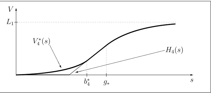
Figure 5. A computer drawing of the payoff function H4(s) and
the value function V4∗(s) , when (1.2.17) holds for L1 and L2.
-6
b∗4 g∗ L1
A
A
A A U
V4∗(s)
9
H4(s) V
s
Figure 6. A computer drawing of the payoff function H4(s) and
[image:25.612.131.469.503.653.2]1.3. Main results and proofs
Taking into account the facts proved above, let us now formulate the main assertions of the chapter. We recall that the price process S of the underlying risky asset is defined in (1.1.1)-(1.1.2), and the exercise boundaries g∗ and h∗ for the underlying perpetual American put and call options are given by (1.1.13).
Proposition 1.3.1 In the optimal stopping problem of (1.1.3), related to the perpetual Amer-ican call-on-call option with strike prices K1 > 0 and K2 > 0 of the outer and inner payoffs,
respectively, the value function has the form
V1∗(s) =
V1(s;b∗1), if s < b ∗ 1 (s−K2)−K1, if s ≥b∗1
(1.3.1)
where the function V1(s;b∗1) and the hitting boundary b∗1 ≥h∗ for the right-hand optimal exercise
time τ1∗ in (1.1.16) are given by (1.2.4) (see Figure 1 above).
Proposition 1.3.2 In the optimal stopping problem of (1.1.4), related to the perpetual Amer-ican call-on-put option with strike prices 0< K1 < L2 of the outer and inner payoffs,
respec-tively, the value function has the form
V2∗(s) =
V2(s;a∗2), if s > a ∗ 2 (L2 −s)−K1, if s≤a∗2
(1.3.2)
where the function V2(s;a∗2) and the hitting boundary a∗2 ≤g∗ for the left-hand optimal exercise
time τ2∗ in (1.1.16) are given by (1.2.7) (see Figure 2 above), while V2∗(s) = 0 and τ2∗ = 0
whenever K1 ≥L2.
Proposition 1.3.3 In the optimal stopping problem of (1.1.5), related to the perpetual Amer-ican put-on-call option with strike prices L1 > 0 and K2 >0 of the outer and inner payoffs,
respectively, the following assertions hold:
(i) if (1.2.10) holds for L1 and K2 then the value function has the form:
V3∗(s) =
V3(s;a∗3, h∗), if s > a∗3 L1−(h∗/γ+)(s/h∗)γ+, if s≤a∗3
(1.3.3)
where the function V3(s;a∗3, h∗) and the hitting boundary a∗3 < h∗ for the left-hand optimal
(ii) if (1.2.13) holds for L1 and K2 then the value function has the form:
V3∗(s) =
V3(s;a∗3), if s > a ∗ 3 L1−(s−K2), if h∗ ≤s≤a∗3 L1−(h∗/γ+)(s/h∗)γ+, if s < h∗
(1.3.4)
where the function V3(s;a∗3) and the hitting boundary a ∗
3 for the left-hand optimal exercise time τ3∗ in (1.1.16) are given by (1.2.14) (see Figure 4 above).
Proposition 1.3.4 In the optimal stopping problem of (1.1.6), related to the perpetual Amer-ican put-on-put option with strike prices L1 > 0 and L2 > 0 of the outer and inner payoffs,
respectively, the following assertions hold:
(i) if (1.2.17) holds for L1 and L2, then the value function has the form
V4∗(s) =
V4(s;b∗4, g∗), if s < b ∗ 4 L1+ (g∗/γ−)(s/g∗)γ−, if s≥b∗4
(1.3.5)
where the function V4(s;b∗4, g∗) and the hitting boundary b∗4 > g∗ for the right-hand optimal
exercise time τ4∗ in (1.1.16) are given by (1.2.18) and (1.2.19), respectively (see Figure 5 above); (ii) if (1.2.20) holds with L1 < L2, then the value function has the form
V4∗(s) =
V4(s;b∗4), if s < b∗4 L1−(L2−s), if b∗4 ≤s≤g∗ L1+ (g∗/γ−)(s/g∗)γ−, if s > g∗
(1.3.6)
where the function V4(s;b∗4) and the hitting boundary b ∗
4 for the right-hand optimal exercise
time τ4∗ in (1.1.16) are given by (1.2.21) (see Figure 6 above), while V4∗(s) = L1 −(L2−s)
and τ4∗ = 0 whenever L1 ≥L2.
Since all the assertions formulated above are proved using similar arguments, we only give a proof for the problem related to the perpetual American put-on-call option, which represents the most complicated and informative case.
(1.3.3) or (1.3.4). Applying the local time-space formula from [91] (see also [97; Chapter II, Section 3.5] for a summary of the related results as well as further references) and taking into account the smooth-fit condition in (1.1.21) and the smoothness of the functions in (1.1.10)-(1.1.11), the following expressions
e−rtV3(St) =V3(s) +
Z t
0
e−ru(LV3−rV3)(Su)I(Su 6=a∗3)du+Mt (1.3.7) e−rtW(St) =W(s) +
Z t
0
e−ru(LW −rW)(Su)I(Su 6=h∗)du+Nt (1.3.8) hold, where I(·) denotes the indicator function and the processes M = (Mt)t≥0 and N = (Nt)t≥0 defined by
Mt=
Z t
0
e−ruV30(Su)σSudBu and Nt =
Z t
0
e−ruW0(Su)σSudBu (1.3.9)
are continuous square integrable martingales with respect to the probability measure P. The latter fact can easily be observed, since the derivatives V30(s) and W0(s) are bounded functions. By means of straightforward calculations similar to those of the previous section, it can be verified that the conditions of (1.1.23) and (1.1.24) hold with a∗3 given by either (1.2.12) or (1.2.14). These facts together with the conditions in (1.1.19)-(1.1.20) and (1.1.22) yield that (LV3 −rV3)(s)≤ 0 holds for all s 6=a3∗, and V3(s) ≥ (L1 −W(s))+ is satisfied for all s > 0. It is well known (see, e.g. [105; Chapter VIII, Section 2a]) that (LW −rW)(s) ≤0 holds for all s6=h∗, and W(s)≥(s−K2)+ is satisfied for all s >0. Moreover, since the time spent by the process S at the boundaries a∗3 and h∗ is of Lebesgue measure zero, the indicators which appear in the integrals of (1.3.7)-(1.3.8) can be ignored. Hence, it follows from the expressions in (1.3.7)-(1.3.8) that the inequalities
e−r(τ∧t)(L1−W(Sτ∧t))+ ≤e−r(τ∧t)V3(Sτ∧t)≤V3(s) +Mτ∧t (1.3.10) e−r(ζ∧u)(Sζ∧u−K2)+≤e−r(ζ∧u)W(Sζ∧u)≤e−r(τ∧t)W(Sτ∧t) +Nζ∧u−Nτ∧t (1.3.11)
hold for all 0 ≤ t ≤ u and any stopping times 0 ≤ τ ≤ ζ of the process S started at s > 0. Then, taking the (conditional) expectations with respect to P in (1.3.10)-(1.3.11), by means of Doob’s optional sampling theorem (see, e.g. [79; Theorem 3.6] or [69; Chapter I, Theorem 3.22]), we get that the inequalities
E
e−r(τ∧t)(L1 −W(Sτ∧t))+
≤E
e−r(τ∧t)V3(Sτ∧t)
≤V3(s) +E
Mτ∧t
=V3(s) (1.3.12) Ee−r(ζ∧u)(Sζ∧u−K2)+
Fτ∧t
≤Ee−r(ζ∧u)W(Sζ∧u)
Fτ∧t
(1.3.13)
≤e−r(τ∧t)W(Sτ∧t) +E
Nζ∧u−Nτ∧t
Fτ∧t
hold for all s > 0. Thus, letting u and then t go to infinity and using (conditional) Fatou’s lemma, we obtain
Ee−rτ(L1−W(Sτ)) ≤Ee−rτ(L1−W(Sτ))+≤Ee−rτV3(Sτ)≤V3(s) (1.3.14) Ee−rζ(Sζ−K2)+
Fτ
≤Ee−rζW(Sζ)
Fτ
≤e−rτW(Sτ) (P-a.s.) (1.3.15)
for any stopping times 0 ≤ τ ≤ ζ and all s > 0. By virtue of the structure of the stopping times in (1.1.16) and (1.1.17), it is readily seen that the equalities in (1.3.14)-(1.3.15) hold with τ3∗ and ζ3∗ instead of τ and ζ, when s≤a∗3 and Sτ3∗ ≥h∗ (P-a.s.).
It remains to be shown that the equalities are attained in (1.3.14)-(1.3.15) when τ3∗ and ζ3∗ replace τ and ζ, respectively, when s > a∗3 and Sτ3∗ < h∗ (P-a.s.). By virtue of the fact that the function V3(s;a∗3, h∗) and the boundary a
∗
3 satisfy the conditions in (1.1.19) and (1.1.20) as well as for the function W(s) and the boundary h∗ the condition (LW−rW)(s) = 0 is satisfied
for s < h∗ and W(h∗−) = h∗−K2 holds, it follows from the expressions in (1.3.7)-(1.3.8) and the structure of the stopping times τ3∗ and ζ3∗ in (1.1.16) and (1.1.17) that the equalities
e−r(τ3∗∧t)V
3(Sτ3∗∧t) =V3(s) +Mτ3∗∧t (1.3.16) e−r(ζ3∗∧u)W(S
ζ∗
3∧u) =e
−r(τ∗
3∧t)W(S
τ∗
3∧t) +Nζ3∗∧u −Nτ3∗∧t (1.3.17)
are satisfied for all 0≤t ≤u, when s > a∗3 and Sτ∗
3 < h∗ (P-a.s.), and where the processes M
and N are defined in (1.3.9). Taking into account the fact that V3(s) is bounded by L1 from above and the properties of the function W(s) in (1.1.11) (see, e.g. [105; Chapter VIII, Sec-tion 2a]), we conclude from (1.3.16)-(1.3.17) that the variables e−rτ3∗V
3(Sτ∗
3) and e
−rζ3∗W(S ζ∗
3)
are equal to zero on the events {τ3∗ =∞} and {ζ3∗ =∞} (P-a.s.), respectively, and the pro-cesses (Mτ∗
3∧t)t≥0 and (Nζ3∗∧t)t≥0 are uniformly integrable martingales. Therefore, taking the
(conditional) expectations with respect to P and letting u and then t go to infinity, we apply the (conditional) Lebesgue dominated convergence theorem to obtain the equalities
E
e−rτ3∗(L
1−W(Sτ∗ 3))
=E
e−rτ3∗(L
1−W(Sτ∗ 3))
+
=E
e−rτ3∗V
3(Sτ∗ 3)
=V3(s) (1.3.18) Ee−rζ3∗(S
ζ∗3 −K2)+
Fτ∗
3
=Ee−rζ3∗W(S
ζ3∗)
Fτ∗
3
=e−rτ3∗W(S
τ3∗) (P-a.s.) (1.3.19)
for all s > a∗3 and Sτ3∗ < h∗ (P-a.s.). The latter, together with the inequalities in
(1.3.14)-(1.3.15), imply the fact that V3(s) coincides with the function V3∗(s) from (1.1.5), and τ3∗ and ζ3∗ from (1.1.16) and (1.1.17) are the optimal stopping times.
1.3.3 above, one should not stop the underlying process when s > a∗3 holds, one should exercise the initial option only when either s≤a∗3 under (1.2.10) or s < h∗ under (1.2.13) is satisfied, while both the initial and underlying options should be exercised immediately whenh∗ ≤s≤a∗3 holds under (1.2.13). Similarly, in the case of put-on-put option in Proposition 1.3.4 above, one should not stop the underlying process when s < b∗4, one should exercise the initial option only when either s ≥ b∗4 under (1.2.17) or s > g∗ under (1.2.20) is satisfied with L1 < L2, while both the initial and underlying options should be exercised immediately when b∗4 ≤ s ≤ g∗ holds under (1.2.20) with L1 < L2.
1.4. Chooser options
In this section, we give a formulation of the perpetual American chooser option optimal stopping problem and prove the uniqueness of solution of the associated free-boundary problem.
1.4.1. Formulation of the problem. Let us finally consider the perpetual American
chooser option which is a contract giving its holder the right to decide at an exercise time τ whether the initial compound option acts further as the underlying perpetual American put or call option. Then, according to the arguments above, the rational price of such a contingent claim is given by the value of the optimal stopping problem
V∗(s) = sup τ
Ee−rτ U(Sτ)∨W(Sτ)
(1.4.1)
where the supremum is taken over the stopping times τ of the process S started at s >0, and x∨y denotes the maximum max{x, y} of any x, y ∈ R. Recall that the functions U(s) and W(s) represent the rational prices of the underlying perpetual American put and call options defined in (1.1.9), respectively. By virtue of the structure of the resulting convex and strictly monotone value functions in (1.1.10)-(1.1.11), we further search for an optimal stopping time in the problem of (1.4.1) of the form
τ∗ = inf{t ≥0|St∈/ (p∗, q∗)} (1.4.2)
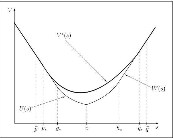
for some numbers 0 < p∗ < c < q∗ < ∞ to be determined, where c denotes the point of intersection of the curves associated with the functions U(s) and W(s) (see Figure 8 below). Note that the latter inequalities always hold, since we have U0(c−)< 0< W0(c+), so that it is never optimal to exercise the option at s =c (see, e.g. [24; Section 4] or [47; Section 3]).
formulate the free-boundary problem
(LV)(s) = rV(s) for p < s < q (1.4.3)
V(p+) =U(p) and V(q−) = W(q) (instantaneous stopping) (1.4.4)
V0(p+) =U0(p) and V0(q−) = W0(q) (smooth fit) (1.4.5)
V(s) = U(s)∨W(s) for s < p and s > q (1.4.6)
V(s)> U(s)∨W(s) for p < s < q (1.4.7)
(LV)(s)< rV(s) for s < p and s > q (1.4.8) for some 0< p < c < q < ∞ fixed.
1.4.2. Solution of the free-boundary problem. In order to solve the free-boundary problem in (1.4.3)-(1.4.8), we first recall that the general solution of the differential equation in (1.4.3) has the form of (1.2.1) with some arbitrary constants C+ and C−. Hence, applying the instantaneous stopping conditions from (1.4.4) to the function in (1.2.1), we obtain the equalities
C+pγ+ +C−pγ− =U(p) and C+qγ+ +C−qγ− =W(q) (1.4.9) which hold for some 0 < p < c < q < ∞, where c is uniquely determined by the equation U(c) = W(c). Solving the system of equations in (1.4.9), we obtain the function
V(s;p, q) =C+(p, q)sγ+ +C−(p, q)sγ− (1.4.10)
which satisfies the system in (1.4.3)-(1.4.4) with
C+(p, q) =
U(p)qγ−−W(q)pγ−
pγ+qγ−−qγ+pγ− and C−(p, q) =
W(q)pγ+ −U(p)qγ+
pγ+qγ−−qγ+pγ− (1.4.11)
for 0 < p < c < q < ∞. Applying the smooth-fit conditions from (1.4.5) to the function in (1.4.10), we obtain the equalities
C+(p, q)γ+pγ+ +C−(p, q)γ−pγ− =p U0(p) (1.4.12) C+(p, q)γ+qγ+ +C−(p, q)γ−qγ− =q W0(q) (1.4.13)
which hold with C+(p, q) and C−(p, q) given by (1.4.11). It is shown by means of standard arguments that the system in (1.4.12)-(1.4.13) is equivalent to
I+(p) = J+(q) and I−(p) = J−(q) (1.4.14)
with
I+(p) = pU
0(p)−γ −U(p)
pγ+ and J+(q) =
qW0(q)−γ−W(q)
qγ+ (1.4.15)
I−(p) =
γ+U(p)−pU0(p)
pγ− and J−(q) =
γ+W(q)−qW0(q)
for all 0 < p < c < q <∞.
In order to show the existence and uniqueness of a solution of the system of equations in (1.4.14), we follow the schema of arguments from [47; Section 4] which are based on the idea of the proof of the existence and uniqueness of solutions applied to the systems of equations in (4.73)-(4.74) from [104; Chapter IV, Section 2] and (3.16)-(3.17) from [42; Section 3]. For this, we observe that, for the derivatives of the functions in (1.4.15)-(1.4.16), the expressions
I+0 (p) =−(γ+−1)(γ−−1)p−γ+γ−L2
pγ++1 ≡ −
(γ+−1)(γ−−1)(p−L2)
pγ++1 <0 (1.4.17)
J+0 (q) = (γ+−1)(γ−−1)q−γ+γ−K2
qγ++1 ≡
(γ+−1)(γ−−1)(q−K2)
qγ++1 <0 (1.4.18)
I−0 (p) = (γ+−1)(γ−−1)p−γ+γ−L2
pγ−+1 ≡
(γ+−1)(γ−−1)(p−L2)
pγ−+1 >0 (1.4.19)
J−0 (q) =−(γ+−1)(γ−−1)q−γ+γ−K2
qγ−+1 ≡ −
(γ+−1)(γ−−1)(q−K2)
qγ−+1 >0 (1.4.20)
hold under 0< p < g∗ < L2 and K2 < h∗ < q <∞, and are equal to zero otherwise, where we set
L2 =
γ+γ−L2 (γ+−1)(γ−−1)
≡ rL2
δ and K2 =
γ+γ−K2 (γ+−1)(γ−−1)
≡ rK2
δ . (1.4.21)
Hence, the function I+(p) decreases on the interval (0, g∗) from I+(0+) = ∞ to I+(g∗) = 0, and then remains equal to zero on the interval (g∗,∞), so that the range of its values is given by the interval (0,∞). The function J+(q) is equal to J+(h∗) = (γ+ −γ−)h1∗−γ+/γ+ > 0 on the interval (0, h∗), and then decreases to zero on the interval (h∗,∞), so that the range is (0, J+(h∗)). The function I−(p) increases from zero to I−(g∗) = (γ−−γ+)g
1−γ−
∗ /γ− >0 on the interval (0, g∗), and then remains equal to I−(g∗) on the interval (g∗,∞), so that the range is (0, I−(g∗)). The function J−(q) is equal to zero on the interval (0, h∗), and then increases from J−(h∗) = 0 to infinity on the interval (h∗,∞), so that the range is (0,∞). It is shown by means of straightforward computations that I+(g∗∧c)< J+(h∗∨c) and I−(g∗∧c)> J−(h∗∨c) holds. This fact guarantees that the ranges of values of the left- and right-hand sides of the equations in (1.4.14) have nontrivial intersections.
It thus follows from the left-hand equation in (1.4.14) that, for each q ∈ (h∗ ∨ c,∞), there exists a unique number p ∈ (p, gb ∗ ∧c), where pb is uniquely determined by the equa-tion I+(p) =b J+(h∗∨c). It also follows from the right-hand equation in (1.4.14) that, for each
p∈(0, g∗∧c), there exists a unique number q∈(h∗∨c,q), whereb qbis uniquely determined by the equation I−(g∗∧c) = J−(bq) (see Figure 7 below). We may therefore conclude that the equations in (1.4.14) uniquely define the function q+(p) on (p, gb ∗∧c) with the range (h∗∨c,∞) and the
that together with the inequalities h∗∨c≡q+(p)b ≡q−(0+)< q−(g∗∧c) <∞ ≡q+(g∗)
guar-antees the existence of exactly one intersection point with the coordinates p∗ and q∗ of the curves associated with the functions q+(p) and q−(p) on the interval (p, gb ∗ ∧ c) such that
h∗∨c < q+(p∗)≡q∗ ≡q−(p∗)<qbholds (see Figure 7 below). This completes the proof of the
claim.
-6
b
p p∗ g∗ L2
K2
h∗
q∗
b q
XX XX
XX XX
XXXz q+(p)
@ @ @ @ @ @ @ @ I
q−(p)
q
[image:33.612.125.425.470.710.2]p
Figure 7. A computer drawing of the functions q+(p) and q−(p) .
-6
b
p p∗ g∗ c h∗ q∗ bq
@ @
@ @
@ @
@ @@R V∗(s)
H H H H H H Y
W(s)
1 U(s)
V
s
Summarising the facts proved above, we are now ready to formulate the following result.
Proposition 1.4.1 Let the process S be given by (1.1.1)-(1.1.2), the functions U(s) and W(s)
be defined in (1.1.9)-(1.1.11), and the number cis uniquely determined by U(c) = W(c). Hence, in the optimal stopping problem of (1.4.1), related to the perpetual American chooser option with the inner put and call payoffs with strike prices L2 >0 and K2 >0, respectively, the value
function has the form
V∗(s) =
V(s;p∗, q∗), if p∗ < s < q∗
U(s)∨W(s), if s ≤p∗ or s≥q∗
(1.4.22)
where the function V(s;p, q) is given by (1.4.10)-(1.4.11), and the exit boundaries p∗ and q∗
such that 0 < p∗ < g∗ ∧c ≤ h∗∨c < q∗ < ∞ for the optimal exercise time τ∗ in (1.4.2) are
uniquely determined by the system of (1.4.14) (see Figure 8 above). The underlying perpetual American put or call option should then be exercised at the same time τ∗.
Proof of Proposition 1.4.1. In order to verify the assertion stated above, let us follow the schema of arguments from [47; Theorem 3.1] and show that the function defined in (1.4.22) coincides with the value function in (1.4.1), and that the stopping time τ∗ in (1.4.2) is optimal with the boundaries p∗ and q∗ specified above. Let us denote by V(s) the right-hand side of the expression in (1.4.22). Applying the local time-space formula from [91] and taking into account the smooth-fit conditions in (1.4.5), the following expression
e−rtV(St) = V(s) +
Z t
0
e−ru(LV −rV)(Su)I(Su 6=p∗, Su 6=q∗)du+Mt∗ (1.4.23) holds for all t≥0, where the process M∗ = (Mt∗)t≥0 defined by
Mt∗ =
Z t
0
e−ruV0(Su)σSudBu (1.4.24)
is a continuous square integrable martingale with respect to P. The latter fact can be easily observed, since the derivative V0(s) is a bounded function.
By means of straightforward computations, it can be verified that the conditions of (1.4.7) and (1.4.8) hold with p∗ and q∗ being a unique solution of the system in (1.4.14). These facts together with the conditions in (1.4.3)-(1.4.4) and (1.4.6) yield that (LV −rV)(s) ≤ 0 holds for any s >0 such that s6=p∗ and s6=q∗, and V(s)≥U(s)∨W(s) is satisfied for all s >0. Moreover, since the time spent by the process S at the boundaries p∗ and q∗ is of Lebesgue measure zero, the indicator which appear in the integral of (1.4.23) can be ignored. Hence, it follows from the expression in (1.4.23) that the inequalities
e−r(τ∧t) U(Sτ∧t)∨W(Sτ∧t)
hold for any stopping time τ of the process S started at s >0. Then, taking the expectations with respect to P in (1.4.25), by means of Doob’s optional sampling theorem, we get that the inequalities
Ee−r(τ∧t) U(Sτ∧t)∨W(Sτ∧t)
≤Ee−r(τ∧t)V(Sτ∧t)
≤V(s) +EMτ∗∧t=V(s) (1.4.26)
hold for all s >0. Hence, letting t go to infinity and using Fatou’s lemma, we obtain
Ee−rτ U(Sτ)∨W(Sτ)
≤Ee−rτV(Sτ)
≤V(s) (1.4.27)
for any stopping time τ and all s > 0. By virtue of the structure of the stopping time in (1.4.2), it is readily seen that the equalities in (1.4.27) hold with τ∗ instead of τ when either s≤p∗ or s≥q∗.
It remains to be shown that the equalities are attained in (1.4.27) when τ∗ replaces τ for p∗ < s < q∗. By virtue of the fact that the function V(s;p∗, q∗) and the boundaries p∗ and q∗ satisfy the conditions in (1.4.3) and (1.4.4), it follows from the expression in (1.4.23) and the structure of the stopping time in (1.4.2) that the equality
e−r(τ∗∧t)V(Sτ∗∧t;p∗, q∗) = V(s) +M∗
τ∗∧t (1.4.28)
is satisfied for all s ∈ (p∗, q∗), where the process M∗ is defined in (1.4.24). Observe that the explicit form of the function in (1.4.10) and (1.4.11) yields that the condition
E
h
sup t≥0
e−r(τ∗∧t)V(Sτ∗∧t;p∗, q∗)
i
<∞ (1.4.29)
holds for all s∈(p∗, q∗), as well as the variable e−rτ
∗
V(Sτ∗;p∗, q∗) is equal to zero on the event
{τ∗ = ∞} (P-a.s.). Hence, taking into account the property in (1.4.29), we conclude from the expression in (1.4.28) that the process (Mτ∗∗∧t)t≥0 is a uniformly integrable martingale.
Therefore, taking the expectation in (1.4.28) and letting t go to infinity, we apply the Lebesgue dominated convergence theorem to obtain the equalities
Ee−rτ∗ U(Sτ∗)∨W(Sτ∗)=Ee−rτ ∗
V(Sτ∗;p∗, q∗) =V(s) (1.4.30)
for all s∈ (p∗, q∗). The latter, together with the inequalities in (1.4.27), implies the fact that V(s) coincides with the value function V∗(s) from (1.4.1) and τ∗ from (1.4.2) is the optimal
stopping time.
Remark 1.4.2 Observe that the system of (1.4.14) is equivalent to the system of (4.5) from [47] with the only difference that the (p, gb ∗∧c) and (h∗∨c,bq) are allowed for p∗ and q∗, respectively,