The Analysis and Simulation of Improved Linearly Interpolative Channel Estimation in LTE System

2017 International Conference on Computer, Electronics and Communication Engineering (CECE 2017) ISBN: 978-1-60595-476-9

The Analysis and Simulation of Improved Linearly Interpolative

Channel Estimation in LTE System

Yung-an KAO and Yu-xiang ZENG

Department of Electrical Engineering Chang Gung University Tao-yuan, Taiwan, ROC

Keywords: LTE, OFDM, Channel estimation.

Abstract. In the previous study, we propose a method to calculate the linear phase factor, and then use it to find the new linear interpolation filter coefficients. This new interpolation filter coefficient can improve the effect of 1-D linear interpolation. But this paper limit the pilot arrangement which is comb-type, and the distance between two pilots is a power of 2. In this paper, we adapt this method for channel estimation in the 3GPP-LTE. This method still has good effect in the LTE even the distance between two pilots is not a power of 2.

Introduction

In wireless communication environment, the transmitted signals are often influenced by the multipath channel. It is necessary for receiver to use equalizer to compensate the multipath channel. In OFDM systems, pilot-based channel estimation is usually adapted, and there are two steps. First step is to estimate frequency response of the pilot subcarriers, the second step is using frequency response of the pilot subcarriers to estimate frequency response of the data subcarriers.

In the OFDM systems, 1-D linear interpolation is the most commonly used channel estimation in the second step. The advantage of 1-D linear interpolation is simple and easier to hardware realization. But when the channel maximum delay becomes large, the effect of the 1-D linear interpolation will decrease. To solve this problem, D. W. Lin [1] proposed the linear phase factor to multiply by the interpolation filter coefficient. In time domain, use the linear phase factor to multiply by the linear interpolation filter coefficient is equal to shifting the 1-D linear phase factor in frequency domain. The appropriate shifting of frequency response will introduce the better performance of the interpolation. But this method [1] uses many statistical calculations, it will have trouble in the hardware realization.

To improve the above problem, Po-Heng Song [2] use the viewpoint of upsampling in discrete-time signal processing [3]. This new algorithm from the upsampling angle is easily to calculate the appropriate linear phase factor. And it has the better performance of the 1-D linear interpolation.

The method [2] did not focus on any wireless communication standards. Its pilot arrangement is comb-type and distance between two pilot subcarriers is a power of 2. But in some wireless communication standards, their distance between two pilot subcarriers are not a power of 2, such as DVB-T [4] and LTE. There are some points which deserve our study when we adopt this method [2] for channel estimation in the 3GPP-LTE system.

We will introduce the pilot arrangement of the LTE in section II. Section III introduces the improved linear interpolation. Section IV presents simulations results and discussion. Section V is the conclusion.

Pilot Arrangement of the LTE

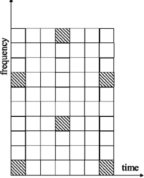
pilot subcarriers is 6. The pilot arrangement is shown as Figure 1. White squares are data subcarriers, and black slash squares are pilot subcarriers. [8] [9].

Figure 1. LTE (long CP) pilot arrangement.

After estimating channel frequency of pilot subcarrier, 2-D linear interpolation can be adopted to estimate the frequency response of data subcarrier. 2-D linear interpolation has two methods, one is do the interpolation on the frequency domain and do the interpolation on the time domain (OFDM symbol) afterwards, and the other is do the interpolation on the time domain (OFDM symbol) and do the interpolation on the frequency domain afterwards. For convenience, we use F-T and T-F to represent these two linear interpolation methods respectively. In the aspect of time, the distance of two pilots is 6 OFDM symbols for T-F and the distance of two pilots is 3 OFDM symbols for F-T. When vehicle speed becomes fast, the effect of F-T is better than the effect of T-F. In the aspect of frequency, the distance of two pilots is 6 subcarriers for F-T and the distance of two pilots is 3 subcarriers for T-F. When channel maximum delay becomes large, the effect of T-F is better than the effect of F-T.

Improved Linear Interpolation

In F-T method, we first assume HF1[k] is the impulse response of linear interpolation filter. Because

the distance between two pilots is 6, HF1[k] will be described to:

1

1 / 6, 6, [ ]

0, otherwise,

F

k k

H k    



We use the linear phase factor to multiply by the interpolation filter coefficient, and the new linear interpolation filter coefficient HN1[k] will be described to:

2 ( )

1[ , ] 1[ ] ,

P k N j

N

N F

H k H k e



    ₍₁₎

where N is the length of an OFDM symbol, NP is the distance between two pilot subcarriers,  is the

shift value of the filter frequency response and k=0, 1, 2…Np-1.

In the time direction, the interpolation in the frequency domain is already done, so we just estimate OFDM symbol which has no pilot subcarriers. The time domain linear interpolation filter coefficient HF2[k]:

2

1 / 3, 3, [ ]

0, otherwise,

F

k k

H k    



Similarly, in T-F method, we first assume HT1[k] is the linear interpolation filter coefficient. HT1[k]

will be described to:

1

1 / 6, 6, [ ]

0, otherwise,

T

k k

H k    



Because HT1[k] is the time domain linear interpolation filter coefficient. We do not multiply by the

linear phase factor. In the frequency direction, the interpolation in the time domain is already done, we just estimate data subcarriers which not known. The frequency domain linear interpolation filter coefficient HT2[k] :

2

1 / 3, 3, [ ]

0, otherwise,

T

k k

H k    



We use the linear phase factor to multiply by the interpolation filter coefficient, and the new linear interpolation filter coefficient HT2[k,] will be described to:

2 ( )

2[ , ] 2[ ] ,

P k N j

N

N T

H k H k e



    ₍₂₎

N is the length of an OFDM symbol, NP is the distance between two pilot subcarriers,  is the shift

value of the filter frequency response and k=0, 1, 2…Np-1.

In the Formula (1) and (2), we can find the appropriate  will improve the effect of linear interpolation. We use formula (3) and 4 step to calculate the error energy. Minimize error energy will obtain the optimal value of τ.

2 /(2 ) 1 0 2 1 1 /(2 ) 2 1 /(2 )

' 1 /(2 ) 1

( ) [ ](1 [ , ] / )

[ ](1 [ , ] / )

[ ] [ , ] / , P P P P N N

err p N P

m N

p N P

m N N N

N N N

p N P

m N N

E H m H m N

H m H m N

H m H m N

                







HN1[m,] is the N point FFT of the linear interpolation filter coefficient HN1[k,]. Define Hp[k] as:

_{[ ], for pilot subcarrier index,}

[ ]

0 , for data and guard band subcarrier index, p

H k k

H k k       [ ]

H k is the channel frequency response which on the pilot subcarrier. Step 1: Calculate the channel responses on pilot subcarrier and obtain Hp[k].

Step 2: Hp[m] is obtained by N point FFT of Hp[k], and first let τ = 0.

Step 3: If Eerr() > Eerr(+1), let =+1 and go back to Step3. If Eerr() < Eerr(+1), then go to Step 4.

Step 4: We have better  now, use formula (1) and (2) to calculate the new linear interpolation filter coefficient HN1[k,] and HN2[k,].

We use method here in detail in [2], we do not discuss here.

Simulation Results and Discussion

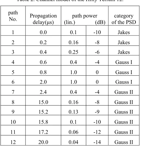
We use time-variant channel which proposed from COST207 [10]. And Table 1 is the simulation parameter. Table 2 is the channel model of the Hilly Terrain 12.

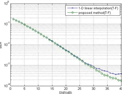
interpolation, and green line is our method. In this simulation environment, our method has a little better than tradition 1-D linear interpolation.

Conclusion

In this paper, we according to pervious improve method for 1-D linear interpolation, we adapt this method for channel estimation in the 3GPP-LTE. In the simulation result, we can find this method is still better than 1-D linear interpolation in the LTE system.

Figure 2. BER simulation results of tradition linear interpolation (F-T), and proposed method (F-T) when vehicle speed is 60km/hr.

Figure 3. BER simulation results of tradition linear interpolation (T-F), and proposed method (T-F) when vehicle speed is 60km/hr.

Table 1. Simulation parameter.

FFT point 2048

Guard interval points 512

Guard band 602~1448

Modulation QPSK

Table 2. Channel model of the Hilly Terrain 12.

path

No. Propagation _{delay(μs) (lin.) (dB)} path power _{of the PSD} category

1 0.0 0.1 -10 Jakes

2 0.2 0.16 -8 Jakes

3 0.4 0.25 -6 Jakes

4 0.6 0.4 -4 Gauss I

5 0.8 1.0 0 Gauss I

6 2.0 1.0 0 Gauss I

7 2.4 0.4 -4 Gauss II

8 15.0 0.16 -8 Gauss II

9 15.2 0.13 -9 Gauss II

10 15.8 0.1 -10 Gauss II

11 17.2 0.06 -12 Gauss II

12 20.0 0.04 -14 Gauss II

References

[1] K.-C. Hung and D.W. Lin, “Optimal Delay Estimation for Phase-Rotated Linearly Interpolative Channel Estimation in OFDM and OFDMA Systems,” IEEE Trans. Signal Process. Letters., Vol. 15, pp. 349-352, 2008.

[2] Y.A. Kao and Po-Heng Song, “The Analysis and Improvement of Linearly Interpolative Channel Estimation in OFDM System,” 2012 International High Speed Intelligent Communication (HSIC 2012), May 2012, pp. 32-35.

[3] Alan V. Oppenheim and Ronald W. Schafer, Discrete-Time Signal Processing. Pearson Prentice Hall, 2010, Third Edition.

[4] ETSI, “Digital video broadcasting (DVB-T); Framing structure, channel coding and modulation for digital terrestrial television,” EN 300 744 Vl.1.2, 1997.

[5] M.-H. Hsieh and C.-H Wei, “Channel Estimation for OFDM Systems Based on Comb-Type Pilot Arrangement in Frequency Selective Fading Channels,” IEEE Trans. Consumer Electronics, vol. 44, no. 1, pp. 217-225, Feb. 1998.

[6] S. Coleri, M. Ergen, A. Puri, and A. Bahai, “Channel Estimation Techniques Based on Pilot Arrangement in OFDM Systems,” IEEE Trans. Broadcast., Vol. 48, No. 3, pp. 223-229, Sept. 2002. [7] F. Said and H. Aghvami, “Linear two dimensional pilot assisted channel estimation for OFDM systems,” in IEE Conf. Telecommunications, Edinburgh, Scotland, Apr. 1998, pp. 32–36.

[8] 3GPP TR 25.814 V7.1.0 (2006-09)( Physical layer aspects for evolved Universal Terrestrial Radio Access (UTRA)).

[9] ETSI TS 136 211 V13.1.0 (2016-04) (Evolved Universal Terrestrial Radio Access (E-UTRA) Physical Channels and Modulation).