AN ENHANCED RULE APPROACH FOR NETWORK INTRUSION DETECTION USING EFFICIENT DATA ADAPTED DECISION TREE ALGORITHM

HYBRID BIG BANG–BIG CRUNCH OPTIMIZATION BASED

OPTIMAL REACTIVE POWER DISPATCH FOR VOLTAGE

STABILITY ENHANCEMENT

Z. ZANDI, E. AFJEI, AND M.SEDIGHIZADEH

Electrical and Computer Engineering Department, Shahid Beheshti University, G.C., Velenjak, Tehran,

1983963113, Iran.

ABSTRACT

One of the most crucial functions in the operation and control of power system is reactive power dispatch (RPD).A hybrid Big Bang–Big Crunch (HBB–BC) optimization algorithm which consists of A Big Bang– Big Crunch algorithm combined with particle swarm optimization (PSO) is proposed in this paper in order to solve optimal reactive power dispatch (ORPD) problem. The L-index of load buses is base for the monitoring methodology for voltage stability. Minimizing the real power loss is the objective. This algorithm is used to find the settings of control variables such as generator voltages, tap positions of tap changing transformers and switchable VAR sources. Furthermore, the optimization models are implemented and solved using the GAMS programming language .The proposed method has been carried out on IEEE 30 -bus test system. For comparative study the results obtained by the proposed algorithm are compared with those obtained by modeling the optimization problem in the GAMS environment. The outcomes indicate that the real power loss is decreased with voltage stability margins increased simultaneously.

Keywords: Particle Swarm Optimization, Reactive Power Dispatch, Voltage Stability ,Big Bang–Big Crunch Algorithm, L-Index

1. INTRODUCTION

Nowadays, reactive power optimization plays a vital role in optimal operation of power systems. There have been many papers by different authors proposed to solve the RPD problem such as Newton approach, linear programming, and interior point methods. Thanks to significant improvement in computers’ capability in recent years, The expert systems [7], fuzzy logic [8], AI approach [9], fuzzy linear programming [10]evolutionary computation techniques such as Genetic Algorithm (GA) [11], Evolutionary Programming (EP) [12] and Evolutionary Strategy [13] have been applied for solving various complex ORPF problems. Increasingly, a major concern in planning and operation of present day power systems is voltage stability. With unmatched generation and transmission capacity expansion, this problem has become very complex due to the continuous growth in the demand for electricity. Stressed system

ISSN: 1992-8645 www.jatit.org E-ISSN: 1817-3195 universe; namely, the Big Bang and Big Crunch

Theory [17]. According to this theory in the Big Bang phase; energy dissipation yields disorder and randomness; while, in the Big Crunch phase, randomly distributed particles are brought back into an order. Motivated by this theory, an optimization algorithm is assembled, which will be called the Big Bang–Big Crunch (BB–BC) method that generates random points in the Big Bang phase and reduces those points to a single representative point through a center of mass or minimization of cost approach in the Big Crunch phase. For improving performance of BB–BC, a hybrid Big Bang–Big Crunch optimization (HBB–BC) is implemented to solve optimization problem. HBB–BC is based on the BB–BC optimization method and the particle swarm optimization (PSO) [18]. The HBB–BC not only considers the center of mass as the average point in the beginning of each Big Bang, but also similar to the approach in particle swarm optimization, utilizes the best position for each particle and the best visited position for all particles. Therefore it causes the performance of the BB–BC approach to improve because of expanding exploration of the algorithm [19]. These unique properties of this novel algorithm encouraged the authors to utilize this method to solve ORPF problems where the purpose is to minimize an objective function which is the real power loss. This algorithm is applied to obtain the optimal control variables so as to improve the voltage stability level of the system in normal and contingency state. The performance of the proposed method has been tested on IEEE 30 bus system. Observations suggest that the proposed method can work more efficiently in both cases, when compared to result obtained by modeling the problem in GAMS environment. This paper is organized as follows: Section 2 introduced voltage stability index. Section 3 provides a concise description and mathematical formulation of ORPF problems. The HBB–BC approach is described in Section 4 together with a short description of the algorithms. Section5 describe implementation of (HBB–BC) in the ORPD problem. Simulation results are presented for different cases in section 6. Finally the General conclusions are drawn in section 7.

2. VOLTAGE STABILITY INDEX

The voltage stability analysis of a power system can be determined by an index of quantifiable voltage stability, there are a variety of indexes that help assess the steady state voltage stability. In our

case, the voltage stability index (L-index) is used [15]. It is based on a load flow analysis and varies in the range between 0 (for no load) to 1 (voltage collapse point).This index is able to evaluate the steady state voltage stability margin of each bus. The bus with the highest L-index value will be the most vulnerable. The L-index calculation for a power system is briefly discussed as follows: If a power system has N number of total bus, 𝑁_Gnumber of PV bus and N_L number of load bus, then the relationship between voltage and current may be represented as:

�𝐼_IG

L�=�

YGG YGL

YLG 𝑌LL� �𝑉 G

VL� (1)

Where

V

_L,

I

_L are the voltage and current at the load buses.

𝑉

G,

𝐼

_Gare the voltage and current vectors at the generator buses.

Rearranging Eq. (1) we obtain

�𝑉L

IG�=�

ZLL FLG

KGL 𝑌GG� �𝐼 L

VG� (2)

Where

FLG=−[𝑌LL]−1[YLG] (3)

The L-indices for a given load condition are computed for all load buses. The equation for the L-index for j-th node can be written as:

𝐿𝑗=�1− ��𝐹𝑗𝑖� |_�𝑉𝑉𝑖| 𝑗� 𝑁𝐺

𝑖=1

∠(Ѳ𝑖𝑗+𝛿𝑖− 𝛿𝑗)� (4)

𝐹𝑗𝑖=�𝐹𝑗𝑖�∠Ѳ𝑖𝑗 (5)

𝑉𝑖= |𝑉𝑖|∠𝛿𝑖 (6)

𝑉𝑗=�𝑉𝑗�∠𝛿𝑗 (7)

The values of F_jiare obtained from the matrix F_LG .The L-index of a bus indicates the proximity of voltage collapse condition of that bus. The indicator 𝐿𝑚𝑎𝑥is used to estimate the distance of the actual

state of the system to the stability limit and considered to be a quantitative measure.

3. PROBLEM FORMULATION

optimization in which case, the objective is to minimize the real power loss. While satisfying equality and inequality constraints, the function is optimized. This is mathematically is represented as follows:

𝑃𝐿𝑜𝑠𝑠= � 𝐺𝑖,𝑗(𝑈𝑖2+𝑈𝑗2−2𝑈𝑖 𝑖,𝑗∈𝑁

𝑈𝑗cos�𝜃𝑖𝑗� (8)

The reactive power optimization problem is subject to the following constraints:

Equality Constraints

The equality constraints are the balance of the active and reactive power described by the set of power flow equations, and are satisfied by running the power flow program. They can be expressed as follows:

(i)PGi−PDi= Vi� Vj( Gijcos�θij�+ Bijsin�θij� j∈Ni

)

i = 1,2, … … … NB−1 (9)

(ii)QGi−QDi= Vi�Vj j∈Ni

�Gijsin�θij� −Bijcos�θij� �

i = 1,2, … … . . NPQ (10)

Where N_PQ andN_B−1, are number of load buses and total number of buses excluding slack bus respectively; P_Gand Q_G are the generator real and reactive power respectively; P_Dand Q_D are the load real and reactive power respectively; Gij and Bij are the transfer conductance and susceptance between bus i and bus j respectively.

Inequality Constraints

The inequality constraints in all of the problems represent the system operating constraints. Generator terminal bus voltages, transformers tap setting, and reactive power generated by the capacitor bank are the control variables which are self – constrained. Voltage stability index of load buses, reactive power generation, load bus voltages, and line flow limit are the state variables whose limit is satisfied in the objective function by penalty coefficients.

(iii) Generator voltages (V_G) and reactive power outputs (Q_G) are restricted by their limits as follows:

QGimin≤QGi ≤QGimax i∈NPV (11)

VGimin≤VGi ≤VGimax i∈NPV (12)

Where, N_PV is number of voltage buses.

(iiii) Load Bus Voltage (VL):

VLimin≤VLi ≤VLimax i∈NPQ (13)

Where, N_PQ is the number of load buses.

(v) Capacitor bank reactive power is limited as follows:

QCimin ≤QCi ≤QCimax i∈NC (14)

Where, NC is the number of capacitor banks.

(vi) Tap settings are restricted as:

tkmin≤tk ≤tkmax i∈NT (15)

Where, N_T is the number of tap-setting transformer branches.

(vii) Line flow limited as follows:

Sl≤Slmax l∈NL (16)

Where, N_L is the number of transmission lines.

(viii) Voltage stability constraint:

Lj≤ 𝐿𝑚𝑎𝑥 j∈NPQ (17)

Where, N_PQ is the number of load buses.

The next section presents the details of proposed approach for solving this particular complex optimization problem.

4. HBB–BC METHOD APPROACHES

4.1. BB–BC

The BB–BC method developed by Erol and Eksin [17] consists of two phases: a Big Bang phase, and a Big Crunch phase. In the Big Bang phase, candidate solutions are randomly distributed over the search space. Erol and Eksin [17] related the random nature of the Big Bang to energy dissipation or the transformation from an ordered state (a convergent solution) to a chaos state (new set of solution candidates).The Big Ban phase is followed by the Big Crunch which is a convergence operator which includes many inputs but only one output Known as the ‘‘center of mass”. The only outcome has been achieved by calculating the center of mass. In here, the term mass refers to the inverse of the fitness function value as mentioned in [20]. The point representing the center of mass is also represented by 𝑥cand is calculated by

𝑥⃗c₌∑

1 𝑓i N i=1

∑ 1

𝑓i N i=1 𝑥⃗

i ₍₁₈₎

Where 𝑥iis a point generated within an

ISSN: 1992-8645 www.jatit.org E-ISSN: 1817-3195 the Big Bang phase. After the Big Crunch phase,

the algorithm must create new members to be used as the Big Bang of the next iteration step which can be done by utilizing the previous knowledge (center of mass) by spreading new off-springs around this center of mass using a normal distribution operation in every direction where the standard deviation of this normal distribution function decreases as the number of iterations of the algorithm increases [20]

𝑥new_=𝑥c₊l.r

k (19)

Where 𝑥cstands for the center of mass, l is the upper limit of the parameter, r is a normal random number and k is the iteration step. Then new point 𝑥new _{is upper and lower bounded. The center of}

mass is recalculated after the second explosion. These consecutive explosion and contraction steps are carried repetitively until a stopping criterion has been met.

4. 2. HBB–BC

In order to improve the exploration ability, this paper uses the potentials of the particle swarm optimization to improve the ability to explore the BB–BC algorithm. The particle swarm optimization is inspired by the social behavior of bird flocking and fish schooling that has a population of individuals, called particles, which sets their movements depending on their own experience as well as the population’s experience [18]. In every iteration, a particle travels towards a direction which is computed from the best visited position (local best) and also the best visited position of all particles in its neighborhood (global best). The HBB–BC method not only uses the center of mass but also utilizes the best position of each candidate (𝑝𝑏𝑒𝑠𝑡_𝑖) as well as the best global position (𝑔𝑏𝑒𝑠𝑡_𝑖 ) to produce a new solution [20],

𝑥_inew(k+1)=𝛼2𝑥ic(k)+ (1− 𝛼2)(𝛼3𝑔𝑏𝑒𝑠𝑡𝑖𝑘

+(1− 𝛼3 )𝑝𝑏𝑒𝑠𝑡𝑖𝑘) +𝑟𝛼1(𝑥

max_{− 𝑥}min₎

k + 1 (20)

Where 𝑟_𝑗is a random number from a standard

normal distribution that changes for each candidate, and 𝛼₁is a parameter for limiting the size of the search space.α2 and α3 are adjustable parameters controlling the influence of the global best and local best on the new position of the candidates, respectively. The agent of a population-based search algorithm performs three steps in every iteration to achieve the concepts of exploration and exploitation: self-adaptation, cooperation and competition. In is noteworthy to mention that in the self-adaptation step, each particle improves its

performance. In the cooperation step, members cooperate with each other by transforming the information. Finally, in the competition stage, members try to compete in order to survive. In the standard BB–BC algorithm, although the cooperation step is satisfied by using the concept of center of mass, the self-adaptation and cooperation steps are not considered to be suitable enough. Adding the potentials of the PSO algorithm will definitely improve these steps. The first term of Eq. (20) represents the cooperation step of the

algorithm. The term related to 𝑝𝑏𝑒𝑠𝑡_𝑖can be

considered as the self-adaptation step of the algorithm that incites particles to improve their solutions, and the competition step is shown by the term related to𝑔𝑏𝑒𝑠𝑡_𝑖. Ultimately, the stochastic form of the algorithm is incorporated by using the last term in the Eq. (20).

5. IMPLEMENTION OF HBB–BC IN THE

ORPD PROBLEM

The implementation of the proposed algorithms for the optimization problem must first include finding the optimal value of control variables namely, generator bus voltages (V_Gi), second the transformer tap-setting (t_k), and finally the reactive power generation (Q_Ci) to minimize the object function while handling the constraints. The implementation process of HBB–BC to the optimal reactive/voltage control problem is described as follows:

Fitness Function: In the reactive power optimization problem under consideration, the objective is to minimize real power loss, satisfying the constraints given by equations (11) to (17). For each particle, the equality constraints given by equations (9) and (10) are satisfied by running Newton-Raphson algorithm. Moreover, the inequality constraints on the control variables are considered in the problem representation itself and the constraints on the state variables are considered by adding a quadratic penalty function to the objective function. With the inclusion of penalty function, the new objective function then becomes:

Minf =𝑃𝐿𝑜𝑠𝑠+ KL� ∆LLj2 NPQ

j=1

+Kv� ∆VLj2+ Kq� ∆QGj2 Ng

j=1 NPQ

+ KF� ∆SLj2 NL

j=1

(25)

where K_L,K_v , K_qand K_F are the penalty factors for voltage stability limit violation, the load bus voltage limit violation, generator reactive power limit violation, and the line flow violation respectively. In the above objective function ∆L_Lj , ∆VLj,∆QGj,∆SLj are defined as:

∆LLj=�

LLj−LmaxLj if LLj> LmaxLj

0 otherwise (26)

∆VLj=�

VLj−VLjmax if VLj> VLjmax

VLjmin−VLj if VLj< VLjmin

0 otherwise

(27)

∆QGj=�

QGj−QmaxGj if QGj> QmaxGj

QminjG −QGj if QGj < QGjmin

0 otherwise

(28)

∆SLj=�SLj−Sj

max _{if S}

Lj> SLjmax

0 otherwise (29)

The HBB–BC approach takes the following steps:

Step 1: Form initial candidates in a randomly. Respect the limits of the search space.

Step 2: By running Newton-Raphson power flow, calculate the fitness values of all the candidate solutions

Step 3: According to (18), find the center of the mass. Best fitness individual can be chosen as the center of mass.

Step 4: According to (20), calculate new candidates around the center of the mass

Step 5:Return to step 2 until a stopping criterion is reached.

6. SIMULATION RESULTS

HBB–BC has been implemented to IEEE 30-bus which is shown in Fig.1. These systems are optimized using the optimal reactive power dispatch method for normal and contingency states for two cases, the first is under base load condition for 100 % load level and the second one is under 125% load level with the incorporation of the

voltage stability limit in both the cases. Simulation performed in MATLAB-7. Also this NLP problems are modeled in GAMS-23.5 [21] and solved using the SNOPT [22] solver.

Fig.1. IEEE 30 Bus System.

ISSN: 1992-8645 www.jatit.org E-ISSN: 1817-3195

6.1.case1(100% load level)

First to obtain the optimal values of the control variables the HBB-BC algorithm was run for the 100 % load level. In this case, the objective is to minimize the real power loss that is calculated to be 𝑃𝐿𝑜𝑠𝑠= 0.1755. By calculating L-index it is found

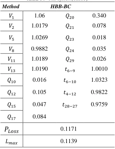
that𝐿_𝑚𝑎𝑥= 0.1435 .Also The optimum settings of the control variables, power loss and 𝐿_𝑚𝑎𝑥for this purpose as obtained from the HBB-BC method and modeling of the problem in GAMS solver are given in Table 1 and Table 2.

It is clear from Table1 and Table 2 that The minimum transmission loss achieved using HBB– BC is 0.1171 which is less in comparison to the result obtained with GAMS solver . The objective function (Ploss) are plotted against the number of iterations in Fig. 2. As depicted in this figure one can readily see the proposed algorithm converges rapidly towards the optimal solution

The voltage profile of the system before and after the application of the HBB–BC algorithm is presented in Fig. 3.Improvement in the voltage profile of the system after the application of the algorithm is evident from this figure.

[image:6.612.328.536.98.605.2]

Fig.2.Objective Function Value Vs Iterations For Case 1

Table 1: Controller settings under base cases for

IEEE 30- bus system(case1) Method HBB-BC

𝑉1 1.06 𝑄20 0.340

𝑉2 1.0179 𝑄21 0.078

𝑉5 1.0269 𝑄23 0.018

𝑉8 0.9882 𝑄24 0.035

𝑉11 1.0189 𝑄29 0.026

𝑉13 1.0190 𝑡6−9 1.0010

𝑄10 0.016 𝑡6−10 1.0323

𝑄12 0.105 𝑡4−12 0.9822

𝑄15 0.047 𝑡28−27 0.9759

𝑄17 0.084

𝑃

𝐿𝑜𝑠𝑠 0.1171

[image:6.612.338.530.121.351.2]

𝐿𝑚𝑎𝑥 0.1139

Table 2: Controller settings under base cases for IEEE 30- bus system(case1)

Modeling with GAMS

𝑉1 1.06 𝑄20 0.043

𝑉2 1.045 𝑄21 0.115

𝑉5 1.013 𝑄23 0.016

𝑉8 1.019 𝑄24 0.029

𝑉11 1.0189 𝑄29 0

𝑉13 1.100 𝑡6−9 0.982

𝑄10 0 𝑡6−10 0.982

𝑄12 0 𝑡4−12 0.948

𝑄15 0.068 𝑡28−27 0.928

𝑄17 0.080

𝑃

𝐿𝑜𝑠𝑠 0.173

𝐿𝑚𝑎𝑥 0.114

0 10 20 30 40 50 60 0.1169

0.1170 0.1171 0.1172 0.1173 0.1174 0.1175 0.1176 0.1177 0.1178 0.1179 0.1180 0.1181 0.1182 0.1183 0.1184 0.1185 0.1186 0.1187 0.1188 0.1189 0.1190

P

los

s(

p.

u)

[image:6.612.90.281.276.524.2]

[image:7.612.103.266.524.690.2]

Fig. 3. Voltage Profile For Case 1 (Base Case).

To investigate the system under disturbance, contingency analysis was conducted. From the contingency analysis, the most severe case is found for line outages (28–27). For these optimal values of control variables Table 3 show the system performance before and after the application of the HBB-BC method when line (28–27) was removed.

By calculating L-index by using optimal values of control variables obtained with GAMS solver it is found that𝐿_𝑚𝑎𝑥 = 0.318 . From Tables 3, it is found that the value of ploss and 𝐿_𝑚𝑎𝑥 decreased and voltage stability has improved after the application of the algorithm. The voltage profile of the system before and after the application of the HBB–BC algorithm under contingency (28–27) is presented in Fig. 4. As it is seen in this figure the voltage profile is improved.

Fig.4. Voltage Profile Under Line Outage 28-27 For Case 1

3 4 6 7 9 10121415161718192021222324252627282930 0.9

0.92 0.94 0.96 0.98 1 1.02 1.04 1.06 1.08 1.1

Before optimization After optimization

Table3: Performance Parameters for IEEE 30- bus system ( Line outage( 28–27) for case 1)

HBB-BC

Before optimization

𝑷

𝑳𝒐𝒔𝒔 𝑳𝒎𝒂𝒙 𝑽𝒎𝒊𝒏

0.1943 0.3762 0.866

After optimization

𝑷

𝑳𝒐𝒔𝒔 𝑳𝒎𝒂𝒙 𝑽𝒎𝒊𝒏

0.1937 0.2939 0.922

3 4 6 7 9 10 12 14 15 1617 18 19 20 2122 23 24 25 2627 28 29 30 0.8

0.85 0.9 0.95 1 1.05 1.1

Before optimization After optimization

V

ol

ta

ge

M

ag

ni

tude

Load Bus NO

V

ol

ta

ge

M

ag

ni

tude

ISSN: 1992-8645 www.jatit.org E-ISSN: 1817-3195 6.1.Case2 (125% load level)

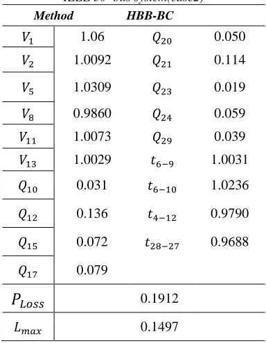
In this case by calculating L-index and the real power loss for the 125 % load level it is found that𝐿_𝑚𝑎𝑥= 0.1884 and 𝑃_{𝐿𝑜𝑠𝑠} = 0.2935.So HBB-BC algorithm implemented for minimizing power loss and voltage stability index. Optimum settings of the control variables, power loss and 𝐿_𝑚𝑎𝑥for this purpose as obtained from the HBB-BC method and modeling of the problem in GAMS solver are given in Table 4 and Table 5.

As seen in Table4 and Table 5 by using HBB–BC algorithm the minimum transmission loss is 0.1912 which is less in comparison to the result obtained with GAMS solver . Also in this case the objective function (Ploss) are plotted against the number of iterations in Fig. 5. As the figure shows, the proposed algorithm converges towards the optimal solution pretty quickly, which an indication of the its efficacy for ORPD problem.AlsoFig.6 illustrates the improvement in the voltage profile of the system after the application of HBB-BC algorithm.

[image:8.612.336.531.115.587.2]

Table 4: Controller settings under base case for

IEEE 30- bus system(case2) Method HBB-BC

𝑉1 1.06 𝑄20 0.050

𝑉2 1.0092 𝑄21 0.114

𝑉5 1.0309 𝑄23 0.019

𝑉8 0.9860 𝑄24 0.059

𝑉11 1.0073 𝑄29 0.039

𝑉13 1.0029 𝑡6−9 1.0031

𝑄10 0.031 𝑡6−10 1.0236

𝑄12 0.136 𝑡4−12 0.9790

𝑄15 0.072 𝑡28−27 0.9688

𝑄17 0.079

𝑃

𝐿𝑜𝑠𝑠 0.1912

𝐿𝑚𝑎𝑥 0.1497

Table 5: Controller settings under base case for IEEE 30- bus system(case2)

Modeling with GAMS

𝑉1 1.06 𝑄20 0.063

𝑉2 1.038 𝑄21 0.178

𝑉5 0.977 𝑄23 0.020

𝑉8 1.014 𝑄24 0.054

𝑉11 1.100 𝑄29 0.039

𝑉13 1.100 𝑡6−9 1.035

𝑄10 0 𝑡6−10 0.988

𝑄12 0 𝑡4−12 0.979

𝑄15 0.103 𝑡28−27 0.932

𝑄17 0.133

𝑃𝐿𝑜𝑠𝑠 0.287

𝐿𝑚𝑎𝑥 0.150

P

los

s(

p.

u)

Iterations

Fig.5.Objective Function Value Vs Iterations For Case 2

0 10 20 30 40 50 60

0.191 0.1911 0.1912 0.1913 0.1914 0.1915 0.1916 0.1917 0.1918 0.1919 0.192 0.1921 0.1922 0.1923 0.1924 0.1925

[image:8.612.89.281.262.509.2]

Fig. 6. Voltage profile for case 2(base case) .

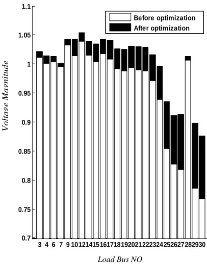
Again a network contingency is considered in this system. From the contingency analysis, the most severe case is found for line outages (28– 27).For optimal values of control variables with GAMS solver it is found that𝐿_𝑚𝑎𝑥= 0.4250.

As

indicated in Table 6 by using the proposed

algorithm when line (28–27) was removed, improvement in voltage stability was achieved and also the value of ploss and 𝐿_𝑚𝑎𝑥 decreased.

[image:9.612.79.291.79.369.2]

Figure 7 show the voltage profile of the system before and after the application of the HBB–BC algorithm under contingency (28–27). As it is evident in this figure there is an improvement in the voltage profile.

Fig.7. Voltage Profile Under Line Outage 28-27 For Case 2

7. CONCLUSIONS

[image:9.612.321.524.169.428.2]

In this paper, the HBB–BC has been successfully implemented to solve ORPF problems. The proposed hybrid BB–BC algorithm considers the combination of the center of mass, the best position of each candidate and the best visited position of all candidates as an average point in the beginning of each Big Bang. The simulation results on IEEE 30- bus test system demonstrate the proposed algorithm is able to improve voltage stability condition along with loss minimization in the normal and contingency situations. The comparison of numerical results of optimal reactive power flow (ORPF) problems with the results obtained by modeling in the GAMS environment, demonstrates the ability of convergence to a better quality solution and possession of superior convergence characteristics of the studied algorithms. These algorithms are demonstrated to give encouraging results for base case and credible contingency conditions.

Table 6: Performance Parameters for

IEEE 30- bus system ( Line outage( 28–27)for case2)

HBB-BC

Before optimization

𝑷

𝑳𝒐𝒔𝒔 𝑳𝒎𝒂𝒙 𝑽𝒎𝒊𝒏

0.3409 0.5828 0.7669

After optimization

𝑷

𝑳𝒐𝒔𝒔 𝑳𝒎𝒂𝒙 𝑽𝒎𝒊𝒏

0.3282 0.3915 0.8759

3 4 6 7 9 10121415161718192021222324252627282930 0.8

0.85 0.9 0.95 1 1.05 1.1

Before optimization After optimization

V

ol

ta

ge

M

ag

ni

tude

3 4 6 7 9 10121415161718192021222324252627282930 0.7

0.75 0.8 0.85 0.9 0.95 1 1.05 1.1

Before optimization After optimization

Load Bus NO

V

ol

ta

ge

M

ag

ni

tude

[image:9.612.88.252.414.577.2]

ISSN: 1992-8645 www.jatit.org E-ISSN: 1817-3195 REFRENCES:

[1] Lee K.Y. Park Y.M. and Ortiz J.L. (1985). “A United Approach to Optimal Real and Reactive Power Dispatch,” IEEE Trans. On Power Apparatus and Systems, Vol.PAS.104, No.5, May, pp 1147-1153

[2] Alsac, O., Bright, J., Prais, M., Scott B. and Marinho, J.L. 990. “Further developments in LP based optimal power flow,” IEEE Transactions on Power Systems, No.5, (1990), pp .697-711.

[3] Sun, D.I., Ashley, B., Brewar, B., Hughes, A. and Tinny, W.F, “Optimal power flow by Newton approach,” IEEE Transactions on Power Apparatus and systems, vol. 103, 1984, pp.2864-2880.

[4] Granville, S., “Optimal reactive power dispatch through interior point methods,” IEEE Transactions on Power Systems,vol. 9,1994, pp. 136-146.

[5] Hong, Y.Y. Sun D.I., Lin S.Y. and Lin, C.J. ,“Multi-year multi-case optimal VAr planning,” IEEE Transactions on Power Systems, vol. 5, 1990, pp.1294-1301.

[6] Lu, F.C. and Hsu, Y.Y.,“ Reactive

power/voltage control in a distribution substation using dynamic programming,” IEE Proceedings on Generation, Transmission and Distribution, vol. 142 , 1995, pp.639-645 [7] Cheng, S.J., Malik O.P., and Hope, G.S, “An

expert system for voltage and reactive power

control of a power system,” IEEE

Transactions on Power Systems, 1988, pp.1449-1455

[8] Abdul Rahman, K.H. and Shahidehpour, S.M., “A fuzzy based optimal reactive power control IEEE Transactions on Power Systems, vol. 8 ,1993, pp. 662-670.

[9] Abdul Rahman K.H., Shahidehpour S.M. and Daneshdoost M ,“ AI approach to optimal VAR control with Fuzzy reactive loads,” IEEE Transactions on Power Systems, vol.10, 1995,pp. 88-97.

[10] Tomsovic, K. 1992 “A fuzzy linear programming approach to the reactive power/voltage control problem ,” IEEE Transactions on Power Systems, vol.7 ,1992,pp. 287-293.

[11] Iba K. “Reactive Power Optimization by Genetic Algorithms,” IEEE Trans on Power Systems, Vol.9, No.2, May1994, pp.685- 692.

[12] Wu Q.H. and Ma J. T. “Power System Optimal Reactive Power Dispatch Using Evolutionary Programming,” IEEE Trans on power system, ,Vol.10.No.3, Aug 1995,pp.1243- 1249. [13] Bhagwan Das, Patvardhan C. “A New Hybrid

Evolutionary Strategy for Reactive Power Dispatch,”Electric Power Research, Vol.65. May 2003, pp.83-90.

[14]1K.Vaisakh, 2P.Kanta Rao. “Differential Evolution Based Optimal reactive power dispatch for voltage stability Enhansment,” JATIT, 2005.

[15] Kessel P, Glavitsch H. “Estimating the voltage stability of power systems,” IEEE Trans Power Syst, vol.1, 1986, pp.346–354. [16] D. Devaraj a, J. Preetha Roselyn,“Genetic

algorithm based reactive power dispatch for voltage stability improvement ” Jurnal of Electrical Power and Energy Systems ,vol.35 December 2010, pp.1151-115.

[17] Erol OK, Eksin I. “New optimization method: Big Bang–Big Crunch, Advances in Engineering Softwar,” vol. 37, February 2006, pp.106–111.

[18]Kennedy J, Eberhart R, Shi Y, “Swarm Intelligence,” Morgan Kaufmann Publishers, 2001.

[19] A. Kaveh, S. Talataharib. “ A Discrete BIG BANG – BIG CRUNCH Algorithm for Optimal Design OF Skeletal Struturesasian,” Journal OF Civil Engineering (Building and hosing ), VOL. 11, NO. 1, 2010, pp. 103-122 [20] A. Kaveha, S. Talataharib.“Size optimization

of space trusses using Big Bang–Big Crunch algorithm,” Elsevier, Computers and Structures ,vol.87, September 2009, pp. 1129– 1140.

[21] Generalized Algebraic Modeling Systems [Online]. Available: wwvw.gams.com.

[22] http://www.gams.com/Solvers/Large Scale

NLP Solvers/ SNOPT

[23] ‘Power system test case archive’, available at: http://