July 31, 2001
SRC
Research
Report
170
Three-Dimensional Web-Based Algorithm
Animations
Marc A. Najork
Marc H. Brown
Systems Research Center
130 Lytton Avenue
Palo Alto, California 94301
Compaq Systems Research Center
SRC’s charter is to advance the state of the art in computer systems by doing basic and applied research in support of our company’s business objectives. Our interests and projects span scalable systems (including hardware, networking, distributed systems, and programming-language technology), the Internet (including the Web, e-commerce, and information retrieval), and human/computer interaction (includ-ing user-interface technology, computer-based appliances, and mobile comput(includ-ing). SRC was established in 1984 by Digital Equipment Corporation.
We test the value of our ideas by building hardware and software prototypes and assessing their utility in realistic settings. Interesting systems are too complex to be evaluated solely in the abstract; practical use enables us to investigate their properties in depth. This experience is useful in the short term in refining our designs and invaluable in the long term in advancing our knowledge. Most of the major advances in information systems have come through this approach, including personal computing, distributed systems, and the Internet.
We also perform complementary work of a more mathematical character. Some of that lies in established fields of theoretical computer science, such as the analysis of algorithms, computer-aided geometric design, security and cryptography, and formal specification and verification. Other work explores new ground motivated by problems that arise in our systems research.
Three-Dimensional Web-Based Algorithm
Animations
Marc A. Najork Marc H. Brown
Marc Brown is currently working at Vendavo Corporation. He can be reached by email at [email protected] or at [email protected].
c
Compaq Computer Corporation 2001
Abstract
Over the past few years, we have developed JCAT, a system for building Web-based collaborative active textbooks on algorithms. JCAT augments the expressive power of Web pages for publishing passive multimedia information with a full-fledged interactive algorithm animation system. Views of a running program can reside on different machines; in an electronic classroom or distance learning setting, a teacher controls the animation, while students view the animation by pointing their Web browsers at the appropriate page.
1
Introduction
This report describes how we have integrated our research on using interactive 3D graphics for algorithm animations [5] with our research on utilizing the Web as a delivery mechanism [6, 7] for algorithm animations.
Interactive, animated 3D graphics is a powerful visualization tool. It adds a level of expressiveness to the display of information, akin to the way that smooth transitions, color, and sound have increased the repertoire available to visualization designers in the past. Pioneering research in the Information Visualizer project at Xerox PARC showed that three-dimensional views help shift the viewing process from being a cognitive task to being a perceptual one. That is, 3D views lever-age the ability of the human perceptual system for discovering patterns, noticing relationships, spotting anomalies, and so on [10, 15].
We have used animated 3D graphics in the Zeus3D system for visualizing the workings of algorithms. In particular, we have used 3D graphics in three funda-mental ways: to capture a history of a two-dimensional view, to unite multiple 2D views of an algorithm, and to express additional fundamental information about structures that are inherently two-dimensional [5]. This report provides a new ani-mation for each of these categories.
Other researchers have also experimented with 3D graphics for animating al-gorithms. Stasko and Wehrli extended the Polka system with a 3D animation li-brary, and used it to produce a number of illuminating 3D algorithm animations. They also provided a taxonomy of the types of displays possible [18]. Two other convincing uses of 3D graphics for algorithm animation were Cox and Roman’s Pavane system [12] and Koike’s VOGUE system [13].
Over the past two decades, we have built a number of algorithm animation sys-tems, most notably BALSA [8], BALSA-II [2], Zeus [3], and Zeus3D [5]. With the advent of the Web, we became interested in integrating our algorithm animations into Web pages. Web pages are ideal for delivering passive multimedia content (text, images, audio, and video), such as a description of an algorithm, whereas applets are well-suited for delivering interactive content, such as an interactive an-imation of an algorithm.
Our first foray into Web-based algorithm animation was the Collaborative Ac-tive Textbook (CAT) system [6], in which algorithm animation applets were em-bedded in Web pages. Animations in CAT were coded in Obliq, a distributed lan-guage, and ran in an Obliq-aware Web browser that we implemented in Modula-3. The main drawback of this work was that it required installing a non-standard Web browser.
Web browser, with no installation.
In addition to enabling users to interactively explore algorithms on their own, JCAT also supports collaborative experiences. The prototypical collaborative set-ting is an electronic classroom, where each student has a computer, slaved in some fashion to the instructor’s machine. Another setting is distance learning, where students are in distributed geographical locations.
In such environments, JCAT allows an instructor to “drive” the algorithm, by providing input data and controlling the execution flow. Students can “attach” their animations to the instructor’s algorithm, thereby yielding control of the execution of the algorithm, but retaining full control over the presentation of the views.
The traditional technique that has been used since the mid-80’s to retrofit algo-rithm animation systems for use in electronic classrooms utilizes shared windows of some sort [1]. Such systems display replicas of the windows on the instructor’s machine on each student’s machine. This approach is easy to implement, because the replication is handled at the window system level, not by the algorithm anima-tion system.
JCAT does not transmit bitmaps from an instructor to each student. The al-gorithm, running on the instructor’s machine, communicates “interesting events” to the views that are running on student machines, and the views on the students’ machines react to the interesting events by updating their displays. The use of “interesting events” has four advantages over a window-sharing design.
First, the student has the ability to interact with the applet and control the way data is presented. Interactive control over the presentation of the views is partic-ularly important in a 3D setting. When viewing 3D scenes on a flat screen, many people have difficulties resolving the ambiguities in the image. Providing inter-active controls, such as moving the virtual camera viewing the scene, or rotating the object being viewed, allows viewers to resolve ambiguities in the images us-ing their hand-eye feedback loop. Such interactive manipulation is essential for leveraging the human perceptual system.
Second, performing animations on each student’s machine is better utilization of network bandwidth. Achieving smooth animations using a window-sharing proach requires the transmission of 10 to 30 bitmaps per second, while our ap-proach only requires the transmission of one interesting event every few seconds.
Third, our approach has the advantage of leveraging the particular hardware characteristics of each machine. For example, if a student’s machine contains a 3D graphics chipset, 3D animations will be able to exploit this hardware.
same algorithm at once. Similarly, a student who is color-blind may choose to visit a web page containing all black-and-white applets. All these views can be driven simultaneously by the algorithm running on the teacher’s machine.
The remainder of this report is organized as follows. The next section pro-vides an overview of the system’s architecture. Section 3 develops an example animation. Section 4 presents more examples of how we have used 3D graphics for algorithm animation. Five of these examples are adaptations from our earlier work; the other three examples (Figures 4, 7, and 8) represent recent work not shown before. Finally, Section 5 offers some concluding remarks.
2
System Architecture
From the user’s point of view, in JCAT there are multiple views of the running pro-gram, and each is updated simultaneously as the program runs. In addition, there is a control panel for starting, pausing, single-stepping, and stopping the animation, for adjusting its speed, and for giving input to the algorithm. Each view in JCAT, as well as the algorithm itself and the control panel, is implemented as an applet. Because JCAT uses Java’s Remote Method Invocation technology [19] to allow ap-plets to communicate with each other, the views of an algorithm can reside on any machine. Thus, in an electronic classroom, the instructor can control an animation on his machine (specifying input, stepping the program to some point, and so on), and each student in the class can see views of the program on their machines by pointing their browsers at the appropriate page.
The framework for animating an algorithm follows the model pioneered by BALSA: strategically important points of an algorithm are annotated with proce-dure calls that generate “interesting events” [9] (e.g. a “swap elements” event in a sorting algorithm). These events are reported to an event manager, which in turn forwards them to all registered views. Each view responds to interesting events by drawing appropriate images.
JCAT’s 2D animation package, modeled after TANGO’s “path-transition” para-digm [17], is based on the metaphor of graphs consisting of vertices and edges, with time-varying visual properties. It is implemented on top of AWT, Java’s low-level 2D graphics library.
The 3D animations in JCAT are implement using Java3D [16], an object-oriented, scene-graph based graphics library that provides simple animation sup-port. We have added powerful higher-level animation constructs modeled after our earlier work in 3D animation [14].
are configured to use Sun’s Java Plug-In [20], rather than the browser’s built-in interpreter. When a user visits a page with such an applet for the first time, an ActiveX control is run which downloads and installs the Java Plug-In. In addition, if Java3D has not been installed yet, the plugin will automatically download and install Java3D.
3
Authoring an Animation
The task of animating an algorithm in JCAT consists of four parts: Defining the interesting events; implementing the algorithm and annotating it with the events; implementing one or more views; and finally, creating web pages that make use of the algorithm and views. The web pages are prepared using HTML; the events, algorithm, and views are implemented in Java.
This section describes the Java-related parts of the authoring process, using Dijkstra’s shortest-path algorithm as an example. Given a directed graph with weighted edges (where W(u, v) is the weight of the edge from u tov), this al-gorithm finds the shortest path from a designated vertex, called thesource, to all other vertices. The length of a path is defined to be the sum of the weights of the edges along the path.
To do this, Dijkstra’s algorithm associates a cost D(u) with each vertex u, indicating the length of the shortest path found so far from the source tou. Initially, this cost will be infinite for all vertices except the source, whose cost will be zero. It also maintains a bit per vertex indicating whether the vertex has been processed or not. The algorithm then repeatedly selects the unprocessed vertexu with the minimal cost, marks it as processed, and lowers the cost of each neighboring vertex
vtoD(u)+W(u, v), provided that this value is indeed lower than the current cost ofv.
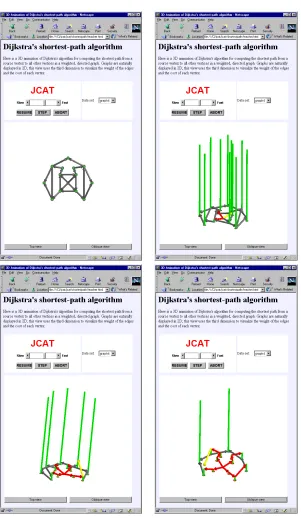
Figure 1 shows an animation of the algorithm. The upper-left image shows the initial graph. This view is actually three-dimensional, and we are viewing it from straight above. From this vantage point, we see that the edges are directed, but we are not able to tell their weights.
The upper-right image, which shows the scene from an oblique viewing angle, reveals this information. Each edge leaves a vertex at height 0, and enters the other vertex at a height proportional to its weight. The cost associated with each vertex is shown as a green column protruding from the vertex. The height of the column is proportional to the cost of the vertex.
cost ofu. Hence, after the lifting is complete, the startpoint of the edge coincides with the tip of the green column aboveu.
If the endpoint of the lifted edge is lower that the green column abovev, this column is lowered to the endpoint, reflecting the lowering of the cost ofvby the algorithm, and the color of the edge changes from yellow to red. Otherwise, the yellow edge simply disappears.
When the algorithm is finished, the graph has been replaced by the shortest-path tree, and the columns above each vertex reflect the length of the shortest shortest-path from the source to that vertex.
This algorithm operates on data that is inherently two-dimensional, given that graphs can be quite naturally drawn in the plane. The third dimension is used to augment the view with additional information; in this case, it is used to represent scalar values, namely the cost of vertices and the weight of edges.
3.1 Specifying the Interesting Events
The first task of the animation author is to specify the set of interesting events that are transmitted from the algorithm to the views, in the form of a Java interface. Ta-ble 1 shows the interface describing the interesting events of Dijkstra’s algorithm. The semantics of the methods in this interface is as follows:
• start(m)is called at the very beginning of the algorithm’s execution; in-dicating that the graph hasmvertices.
• addVertex(u,x,y,d)adds a vertexu to the graph, whereuis an integer identifying the vertex,xand yare its location, anddis its initial cost.
• addEdge(u,v,w)adds an edge fromutovwith weightwto the graph.
• selectVertex(u)indicates thatuwas marked as processed.
• raiseEdge(u,v,d)indicates the additionD(u)+W(u, v); the caller passes D(u)ford.
• lowerDist(u,d)indicates thatD(u)gets lowered tod.
• promoteEdge(u,v)indicates that the edge (u, v)is part of the shortest-path tree.
The Interesting Events
interface ShortestPath { void start(int n);
void addVertex(int u, double x, double y, double d); void addEdge(int u, int v, double w);
void selectVertex(int u);
void raiseEdge(int u, int v, double d); void lowerDist(int u, double d); void promoteEdge(int u, int v); void demoteEdge(int u, int v); }
The Annotated Algorithm
public class Alg extends ShortestPathAlg { public void init() {
super.init();
// create algorithm input panel -- elided }
public void runAlg() {
NumTokenizer ntok = ... // graph data - elided int m = ntok.nextInt(); // num verts start(m);
double[] X = new double[m]; // x coords double[] Y = new double[m]; // y coords double[] D = new double[m]; // cost double[][] W = new double[m][m]; // weight for (int i = 0; i < m; i++) {
X[i] = ntok.nextDouble(); Y[i] = ntok.nextDouble(); D[i] = (i == 0) ? 0.0 : 10.0; addVertex(i, X[i], Y[i], D[i]); }
int n = ntok.nextInt(); // num edges int[] U = new int[n]; // edge start int[] V = new int[n]; // edge end for (int i = 0; i < n; i++) {
int u = U[i] = ntok.nextInt(); int v = V[i] = ntok.nextInt(); W[u][v] = ntok.nextDouble(); addEdge(u, v, W[u][v]); }
boolean[] done = new boolean[m]; for (int iter = 0; iter < m; iter++) {
int u = -1;
double min = Double.POSITIVE_INFINITY; for (int i = 0; i < n; i++) {
if (!done[i] && D[i] < min) { min = D[i];
u = i; } }
done[u] = true; selectVertex(u);
for (int i = 0; i < n; i++) { if (U[i] == u) {
int v = V[i]; raiseEdge(u, v, D[u]); if (D[v] < D[u] + W[u][v]) {
demoteEdge(u, v); } else {
D[v] = D[u] + W[u][v]; promoteEdge(u, v); lowerDist(v, D[v]); } } } } } }
The 3D View
public class View3D extends ShortestPathView3D { DiskGO[] verts;
CylinderGO[] dists; GroupGO[][] edges; int[] parents;
public void start(int m) { verts = new DiskGO[m]; dists = new CylinderGO[m]; parent = new int[m];
for (int i = 0; i < m; i++) parents[i] = -1; edges = new GroupGO[m][m];
scene.flush(); }
public void addVertex(
int u, double x, double y, double d) {
verts[u] = new DiskGO(new Point3(x,y,0), new Point3(0,0,1), 0.2);
scene.add(verts[u]); if (d > 0.0) {
Point3 top = new Point3(x,y,d); dists[u] = new CylinderGO(
new Point3(x,y,0), new PointProp(top), 0.1); SurfaceGO.SetColor(dists[u],"green"); scene.add(dists[u]);
} }
public void addEdge(int u, int v, double w) { Point3 a = verts[u].getCenter(); Point3 b = verts[v].getCenter(); Point3 c = Point3.Plus(b,Point3(0,0,w)); Point3 d = Point3.Minus(c,a);
Point3 e = Point3.Minus(c,Point3.Times(d,0.4)); let grp = new GroupGO();
GO.SetTransform(grp, new TransformProp(Matrix4.Id)); grp.add(new DiskGO(a,d,0.1)); grp.add(new CylinderGO(a,e,0.1)); grp.add(new DiskGO(e,d,0.2)); grp.add(new ConeGO(e,c,0.2)); edges[u][v] = grp;
scene.add(grp); }
public void selectVertex(int u) { SurfaceGO.SetColor(verts[u],"red"); }
public void raiseEdge(int u, int v, double z) { SurfaceGO.SetColor(edges[u][v],"yellow"); Point3 v = new Point3(0,0,z);
GO.GetTransform(edges[u][v]).translate(v,0,2); scene.animate();
}
public void lowerDist(int u, double z) {
PointProp pp = CylinderGO.GetPoint2(dists[u]); Point3 p = pp.get();
pp.linMoveTo(new Point3(p.x,p.y,z),0,2); scene.animate();
}
public void promoteEdge(int u, int v) { SurfaceGO.SetColor(edges[u][v],"red"); if (parents[v] != -1) demoteEdge(parents[v],v); parents[v] = u;
}
public void demoteEdge(int u, int v) { scene.remove(edges[u][v]); }
[image:13.612.104.523.134.649.2]}
The JCAT preprocessor reads theShortestPathinterface and generates a num-ber of Java classes, among themShortestPathAlgandShortestPathView3D. The author then implements the algorithm and view(s) by subclassing these classes.
3.2 Implementing the Algorithm
The animation author implements the shortest-path algorithm by subclassing the
ShortestPathAlgclass that was generated by the JCAT preprocessor, and over-riding the methodsinit and runAlg. Theinit method is responsible for ini-tializing the user interface elements of the algorithm (e.g., to enable the user to provide inputs to the algorithm); for reasons of space, this code is elided. The
runAlgmethod is invoked when the user presses the “run” button in the algorithm control panel. It starts out by obtaining an input data stream from the algorithm input panel (details are elided), and proceeds by initializing the graph and com-puting the shortest path. Note thatrunAlgmakes calls to start, addVertex,
addEdge, etc. These methods are implemented by the superclass; and correspond to the interesting events from section 3.1.
3.3 Implementing a View
JCAT provides animation authors with a powerful animation library that is based on our earlier research in 3D animation [15]. Scenes are composed ofgraphical objects, either primitive ones (such as disks, cylinders, and cones) or complex ones, calledgroups of graphical objects. Attached to a graphical object are properties that govern its appearance, i.e. its location, orientation, color, texture, etc. A property consists of aname (e.g. Cone.Tip) and a value. Property values are time-variant, and provide the basic animation support.
The animation author implements a 3D view by subclassing the Shortest-PathView3Dclass that was generated by the JCAT preprocessor, and overriding the methods corresponding to the eight interesting events.
View3Dintroduces four new fields: verts, an array of disk objects represent-ing the vertices,dists, an array of cylinders representing the costs of the vertices,
edges, an array of arrows (where each arrow is composed of two disks, a cylin-der, and a cone, and aggregated into a group object) representing the edges, and
parents, an array of vertex numbers identifying the parent of each node in the
Thestartmethod is responsible for clearing the scene and for initializing the various fields defined inView3D.
The addVertexmethod adds a new vertex to the scene. Vertices are repre-sented by white disks that lie in the x y plane. Above each vertex, we also show a green column of height d, provided that d is greater than 0. The location of the cylinder’s base is constant, while its top is controlled by an animatable point property value.
The addEdgemethod adds an edge (represented by an arrow) from vertexu to vertexv. The arrow starts at the disk representing u, and ends at the column overvat heightw. An arrow is composed of a cone, a cylinder, and two disks; its geometry is computed based on theCenterproperties of the disks representingu andv.
The selectVertexmethod indicates that vertex u has been marked as pro-cessed by coloringu’s disk red.
TheraiseEdgemethod highlights the edge fromutovby coloring it yellow, and then lifting it up byz. The arrow is moved by calling thetranslatemethod on its transformation property. The animation will start 0 seconds afteranimate
is called, and will take 2 seconds to complete.
ThelowerDistmethod indicates that the costD(u)of vertexu got lowered,
by shrinking the green cylinder representing D(u). This is done by calling the
linMoveTo(“move over a linear path to”) method on thePoint2(“second end-point”) property of the cylinder.
ThepromoteEdgemethod indicates that(u, v), the edge that is currently be-ing highlighted, becomes part of the shortest-path tree. This is indicated by color-ing the edge red. If there already was a red edge leadcolor-ing tov, it is removed from the view.
Finally, thedemoteEdgemethod removes the edge(u, v)from the view.
4
More Examples
This section shows various ways in which we have used interactive 3D graphics in the JCAT system. The example algorithms are: shaker sort; heap sort; quicksort; finding the closest pair in a set of points; inserting points into a space partition-ing tree; findpartition-ing intersection points of a set of horizontal and vertical lines; and constructing a Voronoi diagram.
4.1 Example: Elementary Sorting
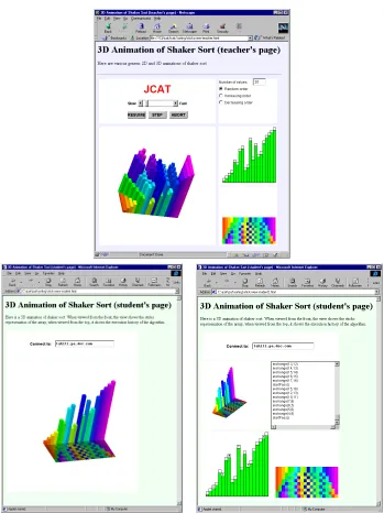
Figure 2 shows how JCAT can be used collaboratively in an electronic classroom. The upper image shows the Web page that a teacher is visiting in his browser; the two images below show the Web browsers of two students at the same time. Al-though the students are viewing different Web pages than the instructor, everyone sees views of the same execution of the algorithm that is running on the instructor’s machine. The views are executing locally on each machine.
The Web page that the instructor is viewing (top image) contains five applets. The JCAT control panel is in the upper left; it allows the instructor to start, single-step, and abort the algorithm, and to control the speed of the animation. The algo-rithm itself is manifested as the applet in the upper right, with various widgets that allow the user to provide data to the algorithm.
Below that is the “Sticks View,” a common 2D representation of an array: each stick represents an element in the array, and the height of the stick is proportional to the value of the element. Whenever two elements of the array are exchanged, the corresponding sticks trade places in a smooth animation. When the array is completely sorted, the sticks will be arranged from short to tall, from left to right.
In the lower right, we see the “Chips View.” This view captures a history of the contents of the array being sorted. A chip represents an element of the array. As in the “Sticks View,” the horizontal position of a chip indicates its position in the array. However, values of array elements are expressed through color rather than height. This frees up one dimension, which has been used to capture a history of the algorithm’s execution. Whenever the algorithm completes an iteration of its outer loop, a copy of the topmost row of chips is drawn on top. Changes to array elements affect the chips in the topmost row only. When the array is sorted, the chips will be sorted from red to violet.
Finally, in the lower left, we see a 3D version of the “Sticks View.” This view combines the strengths of the “Sticks View” and the “Chips View” into a single view. As in the 2D view, exchanging two elements in the array is shown with a smooth animation of the corresponding sticks trading places. Whenever the al-gorithm completes an iteration of its outer loop, the frontmost row of sticks is duplicated. As the algorithm continues, changes are made to the new frontmost row of sticks only. In this way, the “3D Sticks View” combines the elegance of the Sticks View with the Chips View’s capacity for capturing history.
then pulled forward. Thus, the history plane looks exactly like the “Chips View.” The bottom-right image is another student’s Web browser. In addition to the views we have mentioned before, it contains a “Transcript View” containing a tex-tual log of the interesting events.
4.2 Example: Heap Sort
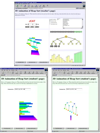
Figure 3 also shows how JCAT can be used in an electronic classroom setting, this lecture being about Heapsort. Recall that Heapsort works in two phases: First, it arranges the elements being sorted into a heap, a complete binary tree in which the value of each node is larger than the values of each of its children. Second, it repeatedly removes the root (i.e., the largest value among the elements) from the heap, sets it aside, and reestablishes the heap property, doing so until the heap is empty.
Heaps can be implemented as arrays by placing the root node at position 1, and for each node at positioni, placing its left child at position 2iand its right child at position 2i+1.
As in the previous example, all three screen dumps were captured at the same time. The upper image shows the instructor’s Web browser; the images below show two students’ Web browsers.
The instructor’s Web page contains six applets: the JCAT control panel; the algorithm input panel; a “Transcript View;” a “Tree View” that shows the heap as a binary tree; a “Sticks View” that shows how the heap is implemented as an array; and a 3D view that combines the tree view and the sticks views. In the Tree View and Sticks View, color is used to distinguish which elements are on the heap and which have been removed.
The 3D view shows a binary tree whose nodes are rods that extend in the z-dimension. As in the sticks view, the length of each rod is proportional to the value of the corresponding heap element. In addition, the rods are color-coded as in Figure 2. It might appear as if color were redundant since the values are already encoded by the lengths of the rods; however, it is quite helpful when the tree is viewed from the front.
In the tree, siblings are not drawn at the same y value; rather, right nodes are slightly lower than their left siblings. More precisely, the y position of each rod corresponds to the index of the corresponding array entry. The effect of this un-conventional layout is that the tree, when viewed from the side, shows the familiar sticks view.
instructor, has rotated the scene in a different way. The student viewing the left image sees the 3D tree as a familiar “Sticks View” (rotated 90 degrees clockwise); the student viewing the right image see the 3D tree as a familiar binary tree; and the instructor views the scene at an oblique angle, thereby revealing both the sticks and binary tree view.
The 3D views have a row of buttons at the bottom. These buttons rotate the scene into various key positions (e.g., a frontal view that reveals the tree, a side view that shows the sticks, and an oblique view that shows both).
The 3D view does not contain any more information than is contained in the two 2D views. However, integrating the two 2D views requires cognitive ef-fort, while obtaining the same information from the single 3D view leverages the viewer’s perceptual system and thereby lessens the cognitive load.
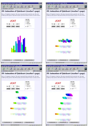
4.3 Example: Quicksort
Figure 4 shows an animation of quicksort. Recall that quicksort is a divide-and-conquer algorithm. An invocation of quicksort proceeds as follows: First, it selects a pivot element. Second, it scans the array from its two endpoints inwards, ex-changing elements from the left side that are larger than the pivot element with elements from the right side that are smaller. Eventually, the two scan pointers meet, meaning that the array has been divided into two parts. All elements in the left part are smaller than the pivot, and all elements in the right are larger. Third, quicksort invokes itself recursively on the two parts.
The four images in Figure 4 are taken at different points during the execution. The upper-left image was taken just after the array was initialized. It shows the familiar sticks view. It also uses the color-coding introduced in Figure 2 to (re-dundantly) express the value of array elements. The sticks view is actually three-dimensional, as can be seen in the following images, which show the scene from an oblique angle.
The upper-right image shows the algorithm during the partitioning phase of the right part of the initial array. The scan pointers are represented by wire cages that surround the array elements that have been scanned. As the scanning proceeds, these cages grow inward until they meet. If you look carefully, you will see that two sticks have left the array and are traveling above it, indicating that the snapshot was taken while an exchange operation was in progress.
placeholder.
From this view, it is easy to see that quicksort can be implemented as an in-place sorting algorithm: Recursive invocations of quicksort manipulate only the opaque part of the array that has been passed to them, and at any point in time, there is only one opaque instance of each array entry.
The lower-left image shows quicksort at the fourth level of recursion, and the lower-right image shows the final unwinding of quicksort’s recursion.
4.4 Example: Closest Pair
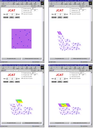
Figure 5 shows an animation of a divide-and-conquer algorithm for finding the closest pair in a set of 2D points.
The algorithm is as follows: First it divides the plane by a line parallel to the y-axis such that each half contains about the same number of points. Next, it recursively finds the closest pair of points in each half. And finally, it merges the two halves, checking if there is a new pair of points (saddling the dividing line) that are closer to each other than the closest pairs found thus far.
The images in Figure 5 show four snapshots of a Web page containing a 3D view of this algorithm as it executes.
The upper-left image shows the initial set of 2D points, viewed from above. The upper-right image shows the initial process of recursively dividing the plane into half-planes until each half-plane contains a single point. The snapshot was captured exactly as the recursion bottomed-out for the first time. At each re-cursive call, the original plane is faded out, and an opaque copy of it is lifted up. It is then split into two halves, and the halves are moved apart slightly. The division process is repeated recursively on the left and right halves.
The two images below show the merge phase, looking for a pair of points, one from each half, that are closer to each other than the closest pair found thus far. The closest pair is highlighted with a red line connecting the two points. The two points from the two half planes that are being checked are temporarily connected by a blue line. The yellow-green region extends to the left and right of the dividing line by the distance of the closest-pair thus far. Only points that lie in this region need to be considered as candidates for a closer pair of points.
After all the candidate points have been considered, the merge phase completes and the merged plane is lowered.
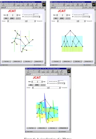
4.5 Example: 2D Tree
Figure 6 shows a visualization of a 2D tree, a space-partitioning tree whose nodes represent points in the plane. This data structure provides support for efficient range searching. A 2D tree is essentially a binary search tree with 2D points in the nodes, using thex and y coordinates of the points as keys in a strictly alternating sequence.
The upper-left image shows the points in the plane. The horizontal and vertical lines indicate the partitioning imposed by nodes in the 2D tree. The long vertical blue line corresponds to the root of the tree; the two horizontal cyan lines corre-spond to its children, and so on. The edges of the 2D tree are displayed as black lines. This representation of a tree resembles the standard layout of a spanning tree, but it does not reveal parent-child relationships.
By contrast, the tree shown in the upper-right image is displayed using a stan-dard binary tree layout, where parent nodes are located above their children. This tree is the result of viewing the scene from the side rather than from the top. The drawback of this viewing angle is that we can no longer see the points in the plane. The image at the bottom shows the scene as viewed from an oblique angle. It simultaneously shows the points in the plane, the walls partitioning the plane that are induced by the nodes of the 2D tree, and the 2D tree.
4.6 Example: Line Intersection
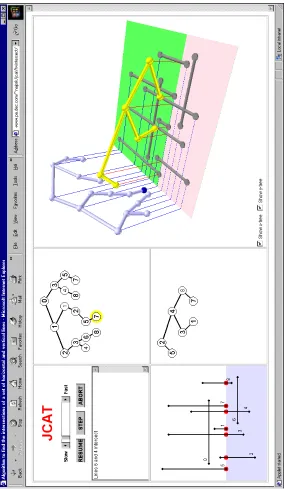
Figure 7 shows an animation of a scan-line algorithm for finding the intersection of horizontal and vertical line segments. The algorithm works by advancing a scan-line from the bottom, stopping each time that it encounters an endpoint of a vertical line or a horizontal line. When the scan-line encounters a horizontal line, the algorithm tests the horizontal line for intersection among all vertical lines touched by the scan-line.
The algorithm uses two binary search trees. First, it builds ay-tree containing they-coordinates of both end-points of each line (horizontal lines contribute only one node to the tree). Next, it performs an in-order traversal of this tree, which corresponds to the scan-line advancing.
When the scan-line touches the lower endpoint of a vertical line, it puts the line’s x-coordinate into a second binary search tree, called the x-tree; when it touches the upper endpoint, the node is removed from thex-tree. When the scan-line touches a horizontal scan-line, it searches thex-tree to find all nodes in the line’s horizontal range. These nodes identify the vertical lines that intersect this horizon-tal line.
The figure contains three 2D views: One view shows the plane containing the line segments along with the scan-line. The second view shows the y-tree, with a highlight surrounding the node currently being visited, corresponding to the loca-tion of the scan-line. The third view shows thex-tree; this tree grows and shrinks as the scan-line progresses. Note that we had to resort to labeling the lines and nodes in order to help the viewer to integrate the three views.
In the 3D view, the two tree views have been drawn orthogonal to the plane view. By aligning the y-tree along the y-axis, we are able to position each node at the same y-coordinate as the line segment endpoint it represents. We have drawn thin grid lines to anchor the tree nodes. Thex-tree is laid out in a similar fashion, that is, thex-coordinate of each node is the same as thex-coordinate of the corre-sponding segment. In addition, the tree moves along with the scan-line, growing and shrinking as vertical line segments are reached and passed.
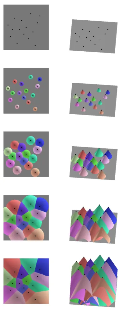
4.7 Example: Voronoi Diagram
A Voronoi Diagram is induced by a set of distinguished points in the plane as follows: Each distinguished point d is surrounded by a polygon whose interior points are closer tod than to any other distinguished point. The Voronoi diagram is simply the union of all these polygons.
Figure 8 shows a filmstrip of an animation that provides an intuitive explanation of this definition. The animation progresses by growing “hills” out of each distin-guished point. In the limit, each hill is the Voronoi polygon of the distindistin-guished point, and the valleys between the hills are the edges of the Voronoi diagram.
The view is implemented by drawing cones (a graphics primitive) centered about the distinguished points and progressively scaling them. Once the cones in-tersect, the hidden surface removal algorithm provided by the underlying graphics package produces the desired effect: when viewed from the top (the left column of Figure 8), we see the Voronoi Diagram, and when viewed from an angle (right column), we see the hills and valleys.
5
Conclusion
This report describes how we have extended JCAT, a Web-based algorithm ani-mation system, with support for interactive 3D aniani-mations. JCAT augments the expressive power of HTML with interactive animations of algorithms in a dis-tributed environment, such as an Electronic Classroom. Since JCAT is based on the “interesting event” paradigm, and since views (including 3D animations) run locally in each student’s Web browser, students can control their views indepen-dently of each other and of the instructor. Interactive control of the viewpoint is crucial for assimilating 3D scenes on a flat display. For this reason, we believe that the JCAT approach is vastly superior to the standard approach of using a shared window system to facilitate an electronic classroom.
This report also has presented a number of examples of ways that 3D graphics can be used for exposing properties of algorithms. Shakersort (Figure 2) shows how the third dimension can be used to capture the history of an algorithm’s exe-cution. Heapsort (Figure 3) shows how two different 2D views can be fused into a single 3D scene. The line intersection algorithm (Figure 7) pushes this idea even further by merging three 2D views. Quicksort (Figure 4) and the closest pair al-gorithm (Figure 5) use the third dimension to illustrate the recursive nature of a divide-and-conquer algorithm directly on its standard visualization. The shortest path algorithm (Figure 1), the 2D tree visualization (Figure 6), and the Voronoi diagram visualization (Figure 8) use the third dimension to show additional infor-mation about structures that are inherently two-dimensional.
Unlike stand-alone algorithm animation systems, JCAT does not require any software installation. Animations are immediately accessible simply by pointing a standard Web browser to a page containing an animation. At first blush, this might seem a minor detail, but we believe it makes a significant difference. Having built a series of stand-alone systems for the past two decades, we learned that installation overhead does deter many potential users. By making the installation completely automatic, we create a seamless user experience. We believe that this technology will expose a much wider audience to algorithm animation.
References
[1] J. Bazik, R. Tamassia, S. P. Reiss, A. van Dam. Software Visualization in Teaching at Brown University. In J. Stasko, J. Domingue, M. H. Brown, B. A. Price (eds.),Software Visualization: Programming as a Multimedia Expe-rience, pages 383-398, MIT Press, 1998.
[2] M. H. Brown. Exploring Algorithms Using Balsa-II.Computer,21(4):14-36, May 1988.
[3] M. H. Brown. Zeus: A System for Algorithm Animation and Multi-view Edit-ing. In1991 IEEE Workshop on Visual Languages, pages 4-9, October 1991.
[4] M. H. Brown, J. Hershberger. Color and Sound in Algorithm Animation. Computer,25(12):52-63, December 1992.
[5] M. H. Brown, M. A. Najork. Algorithm Animation using 3D Interactive Graphics. In ACM Symposium on User Interface Software and Technology, pages 93-100, November 1993.
[6] M. H. Brown, M. A. Najork. Collaborative Active Textbooks.Journal of Vi-sual Languages and Computing,8(4):453-486, August 1997.
[7] M. H. Brown, M. A. Najork, R. Raisamo. A Java-Based Implementation of Collaborative Active Textbooks. In 1997 IEEE Symposium on Visual Lan-guages, pages 376-383, September 1997.
[8] M. H. Brown, R. Sedgewick. A System for Algorithm Animation.Computer Graphics18(3):177-186, July 1984.
[9] M. H. Brown, R. Sedgewick. Interesting Events. In J. Stasko, J. Domingue, M. H. Brown, B. A. Price (eds.),Software Visualization: Programming as a Multimedia Experience, pages 155-171, MIT Press, 1998.
[10] S. K. Card, J. D. MacKinlay, B. Shneiderman (eds.).Readings in Information Visualization : Using Vision to Think. Morgan Kaufmann, 1999.
[11] L. Cardelli. A Language with Distributed Scope. Computing Systems,
8(1):27-59, January 1995.
[13] H. Koike. An Application of Three-Dimensional Visualization to Object-Oriented Programming. In Advanced Visual Interface ’92, pages 180-192, May 1992.
[14] M. A. Najork, M. H. Brown. Obliq-3D: A High-Level, Fast-Turnaround 3D Animation System. IEEE Transactions on Visualization and Computer Graphics,1(2):175-193, June 1995.
[15] G. G. Robertson, S. K. Card, J. D. Mackinlay. Information Visualization Us-ing 3D Interactive Animation. Communications of the ACM, 36(4):56-71, April 1993.
[16] H. Sowizral, K. Rushforth, M. Deering. The Java 3D API Specification. Addison-Wesley, 1997.
[17] J. T. Stasko. TANGO: A Framework and System for Algorithm Animation. IEEE Computer,23(9):27-39, September 1990.
[18] J. T. Stasko, J. F. Wehrli. Three-dimensional Computation Visualization. In 1993 IEEE Symposium on Visual Languages, pages 100-107, August 1993.
[19] Sun Microsystems, Inc. “Remote Method Invocation”.
http://java.sun.com/products/jdk/rmi/
[20] Sun Microsystems, Inc. “Java Plug-In Product”.