DETECTING MOTION BY COMBINING THE STRUCTURE TEXTURE IMAGE DECOMPOSITION AND SPACE TIME INTEREST POINTS

(1)

A NOVEL DIFFERENTIAL EVOLUTION BASED

ALGORITHM FOR HIGHER ORDER NEURAL NETWORK

TRAINING

1_{Y. KARALI,} 2_{SIBARAMA PANIGRAHI,}3_{H. S. BEHERA}

123_{Veer Surendra Sai University Of Technology (VSSUT), Department of Computer Science and}

Engineering, Burla, 768018, Odisha, India

E-mail: [email protected] , [email protected] ,

3_{[email protected]}

ABSTRACT

In this paper, an application of an adaptive differential evolution (DE) algorithm for training higher order neural networks (HONNs), especially the Pi-Sigma Network (PSN) has been introduced. The proposed algorithm is a variant of DE/rand/2/bin and possesses two modifications to avoid the shortcomings of DE/rand/2/bin. The base vector for perturbation is the best vector out of the three randomly selected individuals for mutation, which actually assists intensification keeping the diversification property of DE/rand/2/bin; and novel mutation and crossover strategies are followed considering both exploration and exploitation. The performance of the proposed algorithm for HONN training is evaluated through a well-known neural network training benchmark i.e. to classify the parity-p problems. The results obtained from the proposed algorithm to train HONN have been compared with solutions from the following algorithms: the basic CRO algorithm, CRO-HONNT and the two most popular variants of the differential evolution algorithm (DE/Rand/1/bin and DE/best/1/bin). It is observed that the application of the proposed algorithm to HONN training (DE-HONNT) performs statistically better than that of other algorithms.

Keywords: Artificial Neural Network, Higher Order Neural Network, Pi-Sigma Neural Network,

Differential Evolution, Chemical Reaction Optimization.

1. INTRODUCTION

Conventionally artificial neural network (ANN) models have been applied predominantly to perform pattern matching, pattern recognition and mathematical function approximation. Compared to traditional ANNs, higher order neural networks (HONNs) have several unique features, including: 1) stronger approximation property; 2) faster convergence; 3) greater storage capacity; and 4) higher fault tolerance capability. Thus, HONN models have shown superior performance than traditional ANNs on forecasting, classification and regression problems.

In this paper the class of HONNs and in particular Pi-Sigma Networks (PSNs) has been studied. The PSNs were introduced by Shin and Ghosh [1]. The PSNs have addressed several difficult tasks such as zeroing polynomials [2] and polynomial factorization [3] more effectively than traditional feed-forward neural networks (FNNs). Moreover, PSN employs a less number of weights than other HONNs, but still manages to incorporate the capability of first order HONN indirectly. The efficiency of HONN models depends on the algorithm used for its preparation. The objective of any supervised HONN training is to minimize the

error between the approximation by the HONN and the target output. For this the optimal weight set of a HONN must be obtained. The optimal weight set of a HONN can be obtained by using either gradient or evolutionary learning algorithms. The objective function of HONN training is going to be a multimodal search problem, since it depends on a number of parameters. Thus, the gradient based training algorithms often suffer from several shortcomings, including: 1) easily getting trapped in local minima; 2) has slow convergence properties; 3) training performance is sensitive to initial values of its parameters. Due to these disadvantages, research on different optimization techniques that are dedicated to HONN training is still needed. There are many optimization techniques such as differential evolution (DE) [4], genetic algorithm (GA) [5], particle swarm optimization (PSO) [6], ant colony optimization (ACO) [7], a bee colony optimization (BCO) [8], an evolutionary strategy (ES) [9], quantum inspired algorithms (QEA) [10], chemical reaction optimization (CRO) [11-13] etc. that can be used for HONN training.

(2)

to architecture and mathematical model of PSN; chemical reaction optimization; and differential evolution. The proposed training algorithm for PSN has been explained in Section-3. Experimental results are presented in section-4. And finally concludes in Section-5.

2. RELATED WORKS

2.1 Pi-Sigma Neural Network (PSN)

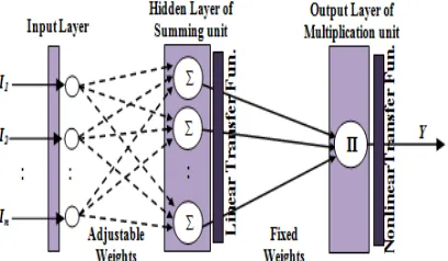
[image:2.612.94.298.589.708.2]

Pi–Sigma Network (PSN) is a feed forward neural network that computes the product of the sum of the input components and passes it to a nonlinear function. The network architecture of PSN (shown in Fig.1) consists of a single hidden layer of summing units and an output layer of product units (instead of summing). The weights connecting the input neurons to the neurons of the hidden layer are adapted during the learning process by the training algorithm, while those connecting the neurons of the hidden layer to the output layer are fixed to one and are not trainable. Such a network topology with only one layer of trainable weights drastically reduces the training time [1, 15-16]. Moreover, the product units of PSN give higher order capabilities which increase its computational power. This is because, the product units enable to expand the input space into higher dimensional space which leads to an easy separation of nonlinearly separable classes where linear separability is possible or a reduction in the proportion of the nonlinearity is achieved. Thus, PSN provides nonlinear decision boundaries offering a better classification capability than the linear neuron (Guler and Sahin, 1994). In addition, Shin and Ghosh (1991) argued that PSNs not only provides a better classification over an extensive class of problems but also require less memory and need at least two orders of less number of computations as compared to MLP for similar performance level.

Figure 1: Architecture of a Typical Pi-Sigma Network

Consider a PSN with NOIN (number of input neurons), NOHN (number of hidden neurons) and one output neuron. The number of hidden neurons in the hidden layer defines the order of a PSN. For a NOHNth order PSN the number of trainable weights is NOIN × NOHN considering each summing unit is associated with NOIN weights. The output of the PSN is computed by making product of the output of NOHN hidden units and passing it to a nonlinear function, which is defined as follows:

)

(

1

∏

=

NOHN

j j

h

Y

σ

Where

σ

a nonlinear transfer function and hj is is the output of jth hidden unit which is computed by making sum of the products of each input (xi) with the corresponding weight (wij) between ith input and jth hidden unit. The output of hidden unit is calculated as follows:

∑

=

NOIN

i

i ij j

w

x

h

1

)

(

2.2 Differential Evolution

(3)

difference vectors used for perturbation of ‘a’ and ‘c’ represents the type of crossover used (bin: binary, exp: exponential). Interested reader may go through [4, 18] to have a detail description regarding DE algorithm and its variants.

Every differential evolution algorithm operates in following steps:

Step 1: Problem and algorithm parameter initialization

Step 2: Initialize the initial population and calculate the fitness of each chromosome/individual

Step 3: Apply Mutation operator to generate the mutant vector

Step 4: Apply crossover between the target vector and mutant vector to generate the trial vector.

Step 5: Perform Selection between trial vector and target vector

Step 6: Termination criteria check if satisfied go to step-7 otherwise go to step-3

Step 7: Use the best individual as the solution of the problem.

2.3 Chemical Reaction Optimization

Chemical reaction optimization (CRO) algorithm was proposed recently by Lam [11], is a variable population-based metaheuristic optimization technique inspired by the nature of chemical reactions. It does not attempt to capture every detail of chemical reaction rather loosely couples chemical reaction with optimization. A chemical reaction is a process that transforms one set of chemical substances (reactants/molecules) to other. Each molecule consists of some atoms and is associated with enthalpy (minimization problem) and/or entropy (maximization problem). During the chemical reaction the intra-molecular structure of a reactant changes. Most of the reactions are reversible in nature. Basing on the number of reactants take part in a reaction, the reaction may be: monomolecular (one reactant takes part in the reaction) or bimolecular (two reactants take part in a chemical reaction) and so on. The major difference between CRO and other evolutionary techniques is that, the population size (that is the number of reactants) may vary from one generation to the other where as in evolutionary techniques the population size remains fixed. But few authors have proposed fixed population sized CRO algorithms and shown that fixed population sized CRO not only performs better but also easier to implement. To have an elaborated description regarding CRO algorithm, interested readers may go through the tutorial of CRO [17].

Every chemical reaction optimization algorithm consists of following steps:

Step 1: Problem and algorithm parameter initialization

Step 2: Setting initial reactants and evaluation of entropy/enthalpy

Step 3: Applying Chemical reactions

Step 4: Reactants update

Step 5: Termination criteria check if satisfied go to step-6 otherwise go to step-3

Step 6: Use the reactant having best enthalpy / entropy as the solution.

3. DE-HONNT METHOD

In this proposed methodology an attempt has been made to combine the advantage of DE/rand/2 and DE/best/2 by overcoming the shortcomings of both the algorithms. The major advantage of DE/rand/2 is diversification i.e. it has less chance to trap to local optima whereas it suffers from exploitation i.e. takes more generations to reach the optimal solution. Compared to DE/rand/2, DE/best/2 is greedier in nature and has faster convergence property. The benefit of fast convergence is obtained by guiding the search with the best solution so far discovered, thereby converging to that point. However, due to guided towards a single solution (i.e. The best solution), in many cases the population may lose its diversity and thereafter gets trapped in a local optimum in a small number of generations.

Taking these facts into consideration to overcome the limitation of slow convergence but reliable DE/rand/2 we use an explorative yet greedy variant of DE/rand/2/bin mutation strategy with novel parameter adaptation. In this algorithm three random individuals are selected from the population for mutation, but out of the three individuals the best individual (i.e. individual with best fitness value) is selected as base vector for perturbation. The other two vectors are used for difference vector. This mutation scheme keeps the intensification property of DE/best/2 (as best out of three individuals is selected as base vector i.e. used to guide the solution) without losing the diversification property of DE/rand/2 (three individuals are selected randomly, avoids premature convergence to a same point and/or to local optima).

(4)

diversifies the solution more as compared to traditional normal or uniform distribution.

Algorithm 1 (DE-HONNT)

Set the iteration-counter i=0

/*Randomly Initialize the population of PopSize individuals: Pg={C1g, C2g , C3g ……., CPopSizeg }, with Cig ={ Wi,1g,…….,Wi,Dg} for i=1,2,3...NP, D=length of each chromosome, Wi,kg=kth gene of ith individual in gth generation representing a weight of PSN.

Evaluate the fitness of each individual

While(termination criteria is not satisfied) do begin % for each individual chromosome (Cig) in the population

for i=1 to PopSize

Select five individuals (I1, I2, I3, I4, I5) and such

that I1≠I2≠I3≠I4≠I5≠i

Sort the five selected individuals

Set r1=best individual out of I1, I2, I3, I4, I5

And rest four are assigned to r2, r3, r4, r5 % Mutation Step

% Generate scale factor

Fi =gaussianrnd (0.5, 0.1), is a random number generated randomly from Gaussian distribution with mean 0.5 and standard deviation 0.1.

for x=1 to D MVk,xg= W

r1,x

g + Fi*( W r2,x

g - W r3,x

g) + Fi*( Wr4,xg - Wr5,xg) end of for

% Generate Cross over Probability

Cri = cauchyrnd(0.7,0.1), is a random number generated randomly from Cauchy distribution with location parameter 0.7 and scale parameter

0.1.It is regenerated if the random number falls out of the range [0-1].

for x=1 to D

if rand(0,1)< Cri TVk,xg = MVk,xg

else

TVk,xg = Wi,xg end of if

end of for

% Selection Step

% Fitness of a chromosome is -1×RMSE on train set

if fitness(TV) > fitness(Cgi) Cig+1= TV

else Cig+1= Cig

end of if end of for

Set the generation counter g=g+1

end of while

The scale parameter (F) is generated randomly from a Gaussian distribution with mean=0.5 and standard deviation=0.1. Here instead of Cauchy distribution, Gaussian distribution is used because it gets most of the numbers within unity due to its short tail property. Moreover, the random numbers generated are not bound within any limit, this is because larger values of scale parameter ‘F’ will assist the solution space to easily escape from large plateaus or suboptimal peaks/valleys, thereby minimizing the chances to trap to local optima.

4. SIMULATION RESULTS

For comparative performance analysis of proposed training method with DE/rand/1/bin, DE/best/1/bin, CRO [14] and CRO-HONNT [22] to train PSN, parity-p problems (p

∈

[3; 6]) have been considered. These problems are widely used benchmarks and are suitable for testing the non-linear mapping and generalization capabilities of training algorithms. The parity-p problem is described as follows: if P represents the number of inputs, and each input can accept values “1” or “−1”, then, the output of the network is “1” if and only if the number of “1” in the inputs of the PSN is odd. Otherwise “−1” occurs in the output of the PSN. Although these problems are easily defined, they are hard to solve, because of their sensitivity to initial weights and possession of a large number of local minima. To classify parity-p (p

∈

[3;6]) problem, PSNs having structure p-p-1 without bias units were considered and trained using proposed method and other methods for comparison. For each parity problem the training set was equal to the testing set and contained 2p patterns.

(5)

conducted 1000 independent simulations using each method for each parity problem. All the simulations were carried out on a system with Intel ® core (TM) 2Duo E7500 CPU, 2.93 GHz with 2GB RAM and implemented using MATLAB (R2009a, The Mathworks, Inc., and Version-7.8.0.347).

The following Tables show the experimental results for parity-p (p

∈

[3; 6]) problems. The table shows Min the minimum number; Mean the mean value; Max the maximum number; and St.D. the standard deviation of the number of training generations and the correct classification percentage. To have a better comparison among the methods, we have performed post hoc analysis and ANOVA on the results obtained from 1000 independent simulations for each problem using each method. The correct classification percentage is computed as follows:

Correct classification (%)=

NOP

C

NOP i i

∑

=1

Where NOP is number of testing patterns (NOP=2p); p- Number of inputs to the PSN; Ci- the coefficient representing the correctness of the classification of the ith testing pattern which is determined as follows:











−

=

−

=

Otherwise

0,

1 T

and

1 Y

when

1,

1 T

and

1 Y

when

,

1 C

_i _i

i i

i

Where Yi and Ti are the output of PSN and target for ith test pattern.

All the training methods gave perfect generalization (100% correct classification) capabilities for parity-3 and 4 problems respectively; hence for these two problems only number of generations to attain the termination criteria was measured.

TABLE 1:Simulation results on parity-3 problem (best results in bold)

Algorithms Generations Mean ± St.D. Min Max

DE-HONNT 1.98 ± 1.40ab ₁ ₁₁

CRO-HONNT 1.86 ± 1.64a 1 12

CRO 2.65 ± 4.03c ₁ ₆₅

DE/rand/1 2.12 ± 1.52b 1 17

DE/best/1 2.11 ± 1.46b ₁ ₉

*Means within a column the same letter(s) are not statistically significant (p=0.05) accordance to Duncan’s Multiple Range Test (SPSS V.16.0.1)

One can see from table-1 and table-2 that for both the problems the proposed method takes

statistically less number of generations to obtain the optimal solutions than the DE variants and basic CRO algorithm. Although the CRO-HONNT takes less number of generations than the proposed method for parity-3 problem but it is not statistically significant to DE-HONNT. Moreover, DE-HONNT takes statistically significantly less number of generations than CRO-HONNT for parity-4 problem.

DE-HONNT 14.36 ± 11.14a ₁ ₉₈

CRO-HONNT 17.41 ± 15.27b ₁ ₁₈₇

CRO 23.04 ± 40.49c ₁ ₉₂₀

DE/rand/1 18.21 ± 15.38b ₁ ₁₉₃

DE/best/1 18.79 ± 15.74b ₁ ₁₆₃

DE-HONNT 108.85 ± 140.33a ₄ ₁₀₀₀

CRO-HONNT 173.61 ± 160.95b ₂ ₁₀₀₀

CRO 194.45 ± 235.14c ₆ ₁₀₀₀

DE/rand/1 245.30 ± 227.84d ₁₀ ₁₀₀₀

DE/best/1 248.62 ± 224.79d ₅ ₁₀₀₀

Algorithms Correct Classification (%) Mean ± St.D. Min Max

DE-HONNT 99.92 ± 0.71c _93.75 ₁₀₀

CRO-HONNT 99.87 ± 0.87bc _93.75 ₁₀₀

CRO 99.67 ± 1.43a _87.50 ₁₀₀

DE/rand/1 99.82 ± 1.03bc _93.75 ₁₀₀

DE/best/1 99.79 ± 1.15b _87.50 ₁₀₀

(6)

DE/best/1/bin and traditional CRO method. However, the proposed method takes statistically less number of generations than other methods to obtain the optimal solutions.

DE-HONNT 256.93 ± 278.34a ₇ ₁₀₀₀

CRO-HONNT 783.49 ± 275.93d 28 1000

CRO 728.97 ± 340.57c ₂₃ ₁₀₀₀

DE/rand/1 535.43 ± 332.98b 29 1000 DE/best/1 547.46 ± 336.36b ₃₀ ₁₀₀₀

Algorithms Correct Classification (%) Mean ± St.D. Min Max

DE-HONNT 97.75 ± 3.20c _81.250 ₁₀₀

CRO-HONNT 97.58 ± 3.20c _81.250 ₁₀₀

CRO 94.02 ± 3.69a _78.125 ₁₀₀

DE/rand/1 95.12 ± 5.52b _78.125 ₁₀₀

DE/best/1 95.21 ± 5.30b _78.125 ₁₀₀

Table-5 and Table-6 show the experimental results for parity-6 problem. None of the methods gave perfect generalization capabilities for parity- 6 problem for all the 1000 simulations. The proposed method not only provides statistically better correct classification percentage but also takes statistically significantly less number of generations to attain the optimal solutions. Although CRO-HONNT method has statistically same correct classification percentage but it takes almost thrice number of generations to attain the solutions.

5. CONCLUSION

In this paper, the Pi–Sigma network which is a special class of higher order neural network has been studied and proposed a novel differential evolution based training algorithm for its training. The use of DE-HONNT method incorporates efficient and effective searching mechanisms, such that it has less chance to trap to local minima and thus enhance the higher order neural network training procedure. Additionally, this method provides the ability to apply them for training “hardware friendly” PSNs, i.e. PSNs with threshold activation functions and small integer weights can

be easily implemented using hardware. The simulation results demonstrate that the proposed training algorithm has superior performance in terms of correct classification percentage (e.g. parity-5, 6) and generations taken to attain the termination criteria (e.g. parity-3,4,5,6) when compared with most popular DE variants, traditional CRO method. Although for some test instances the new training algorithm obtains statistically same solutions (e.g. parity-3 statistically same number of generations and parity-5 statistically same correct classification percentage) but for most of the instances the DE-HONNT methods converges quickly (e.g. parity-4,5,6) and provides statistically better correct classification percentage(e.g. parity-6).

REFRENCES:

[1] Y. Shin and J. Ghosh, “The pi–sigma network: An efficient higher-order neural network for pattern classification and function approximation”, International Joint

Conference on Neural Networks, 1991.

[2] D. S. Huang, H. H. S. Ip, K. C. K. Law and Z. Chi, “Zeroing polynomials using modified constrained neural network approach”, IEEE

Transactions on Neural Networks, Vol. 16, No.

3, 2005, pp. 721–732.

[3] S. Perantonis, N. Ampazis, S. Varoufakis and G. Antoniou, “Constrained learning in neural networks: Application to stable factorization of 2-d polynomials”, Neural Processing Letter,

Vol.7, No. 1, 1998, pp. 5–14.

[4] R. Storn and K.Price, “Differential evolution- A simple and efficient heuristic for global optimization over continuous spaces”, Journal

of Global Optimization, Vol. 11, No.4, 1997,

pp. 341-359.

[5] D. Goldberg, “Genetic Algorithms in Search”,

Optimization and Machine Learning. Reading,

MA: Addison-Wesley (1989).

[6] J. Kennedy, R. C.Eberhart and Y.Shi,“Swarm intelligence”, San Francisco, CA:Morgan

Kaufmann, 2001.

[7] K. Socha and M. Doringo, “Ant colony optimization for continuous domains”,

European Journal of Operation Research, Vol.

185, No. 3, 2008, pp. 1155-1173.

(7)

[9] H.G. Beyer and H.P. Schwefel, “Evolutionary Strategies: A Comprehensive introduction”,

Nat. Comput., Vol. 1, No. 1, 2002, pp. 3-52.

[10]K. H. Han and J.H. Kim, “Quantum-inspired evolutionary algorithm for a class of combinatorial optimization”, IEEE

Transactions on Evolutionary Computation,

Vol. 6, 2002, pp. 580–593.

[11]A. Y. S. Lam and V. O. K. Li, “Chemical-Reaction-inspired metaheuristic for optimization”, IEEE Transactionson on

Evolutionary Computation, Vol. 14, No.3,

2010, pp. 381–399.

[12]A.Y.S. Lam, “Real-Coded Chemical Reaction Optimization”, IEEE Transaction on

Evolutionary Computation, Vol. 16, No. 3,

2012, pp. 339-353.

[13]B. Alatas, “ACROA: Artiﬁcial Chemical Reaction Optimization Algorithm for global optimization”, Expert Systems with

Applications, Vol. 38, 2011, pp. 13170-13180.

[14]J.J.Q. Yu, A.Y.S. Lam and V.O.K. Li, “Evolutionary Artificial Neural Network based on chemical reaction optimization”, in: IEEE Congress on Evolutionary

Computation (CEC), 2011, pp. 2083-2090.

[15]J. Ghosh and Y. Shin, “Efficient higher-order neural networks for classification and function approximation”, in: International Journal on

Neural Systems, Vol. 3, 1992, pp. 323-350.

[16]Y. Shin and J. Ghosh, “Realization of Boolean functions using binary pi-sigma networks”, in: C. H. Dagli, S. R. T. Kumara, Y. C. Shin (Eds.), Intelligent Engineering Systems through

Artificial Neural Networks, ASME Press, 1991,

pp. 205–210.

[17]A. Y. S. Lam, V. O. K. Li, Chemical Reaction Optimization: a tutorial, Memetic Computing

Vol. 4, 2012, pp. 3-17.

[18]S. Das, P. N. Suganthanam, Differential Evolution: A Survey of the state-of-the-Art,

IEEE Transaction on Evolutionary

Computation, Vol. 15, No.1, 2011, pp. 4-31.

[19]M.G. Epitropakis, V.P. Plagianakos, M.N. Vrahatis, Hardware-friendly Higher-Order Neural Network Training using Distributed Evolutionary Algorithms, Applied Soft

Computing, Vol. 10, 2010, pp. 398-408.

[20]S. Das, A. Abraham, U. K. Chakraborty, A. Konar, Differential evolution using a neighbourhood based mutation operator, IEEE

Transaction on Evolutionary Computation,

Vol. 13, No.3, 2009, pp. 526-553.

[21]S. Rahnamayan, H. R. Tizhoosh, M. M. A. Salama, Opposition based differential

evolution, IEEE Transaction on Evolutionary

Computation, Vol. 12, No.1, 2008, pp. 64-79.

[22]K. K. Sahu, S.Panigrahi, H. S. Behera, A Novel Chemical Reaction Optimization algorithm for Higher Order Neural Network Training, Journal of Theoretical and Applied

Information Technology, Vol. 53, No. 3, 2013,