Influential Observations in Stochastic Model of Divisia Index Numbers with AR(1) Errors

(1)

http://dx.doi.org/10.4236/am.2014.56093

Influential Observations in Stochastic Model

of Divisia Index Numbers with AR(1) Errors

Syed Muhammed Aqil Burney1_{, Arfa Maqsood}2

1_{Department of AS&RM, College of Computer Science and Information Systems, Institute of Business}

Management Karachi, Pakistan

2_{Department of Statistics, University of Karachi, Karachi,}_Pakistan

Email: [email protected], [email protected]

Received 31 December 2013; revised 31 January 2014; accepted 8 February 2014

This work is licensed under the Creative Commons Attribution International License (CC BY).

http://creativecommons.org/licenses/by/4.0/

Abstract

We use the general form of hat matrix and DFBETA measures to detect the influential observations in order to estimate the Divisia price index number when the error structure is first order serial correlation. An example is presented with reference to price data of Pakistan. Hat values show the noteworthy findings that the corresponding weights of consumer items have large influence on the parameter estimates and are not affected by the parameter of autoregressive process AR(1). Whereas DFBETAs for Divisia index numbers depend on both the weights and autoregressive pa- rameter.

Keywords

Hat Matrix, DFBETA, Divisia Index Number, Influential Observation, Autoregressive Process

1. Introduction

(2)

the first observation is not always magnificent as suggested by Cochrane and Orcutt [13]. Stemann and Trenkler [14] extended the approach of Puterman [12] to the general linear model with the first order autoregressive er-rors and showed the effect of the presence of a constant term on a leverage point when the correlation of the error term was large in absolute value. Barry et al. [15] extended the study of influential observations to the regression model with AR(2) errors and developed the diagnostic techniques using a hat matrix.

Much literature is on hand on the influential observations diagnostic for the regression models with continu- ous type of regressors. There is a need to have some techniques for finding the influential observations when the dilemma of constructing the index number is concerned. The objective of this paper is to use the analytical tools of hat matrix and DFBETA measures to identify the influential observations in estimating the Divisia price index number.

The paper is organized as follows. Section 2 introduces the Divisia index number model and the role of the initial observation in estimation of model is discussed. The relevant concepts on influence diagnostics for the underlying model are presented in Section 3. An application with reference to Pakistan price data is illustrated in Section 4 and lastly, Section 5 recapitulates the results.

2. Regression Model

The well-known Divisia index number is formulated by the following model

it t it

Dp =α ε+ (1)

where , 1

1

log log log it

it it i t

it

p

Dp p p

p

−

 

= − = _ _

 , log price-change in period t for ith commodity, αt conman trend

in the prices of all commodities at time t (the rate of inflation), and εit is the random component. The errors are assumed to be generated from the first order autoregressive scheme, that is εit =φεi t,−1+uit, where φ <1, and

( )

_it 0,

(

_it _jt

)

2 _ij.

i

E u E u u

w σ δ

= =

This yields the error structure of model (1) as

( )

it 0

E ε = and variance-covariance

(

)

(

)

2 2

1 , 0

i k _k i w k w k σ φ γ

σ φ φ

 − =

 = 

− >

 (2)

Defining more compactly in matrix notation as follows,

( )

2

0,

E ε = E εε′ =σ V

The inverse of variance-covariance matrix can easily be decomposed using cholesky decomposition and can be written as

1

V− =Q Q′

where Q is a lower triangular matrix of order (nT × nT), defined as

2 1

2

1 1

1

1 0 0 0 0 0

0 1 0 0 0 0

0 0 0 0

0 0 0 0 0

(3)

The model (1) is written in matrix form

( 1) ( ) ( 1) ( 1)

P nT nT T T nT

D _× =X _× β _× +ε _× (3)

It is well known that under the above assumption, the best linear unbiased estimator (BLUE) of β in model (1) could be obtained by the generalized least square (GLS) approach as given below

(

₁

) (

1 ₁

)

ˆ

P

X V X X V D

β ₌ _′ − − _′ −

There are different approaches to estimate the parameter vector β, in case of unknown autoregressive parameter φ (see Judge et al. [16]). The value of φ is first estimated from the data using any of the number of suggested alternatives given in Gugarati [17]. The transformation of the vector DP and the design matrix X to the new vector DP QDˆ P

∗ ₌

and matrix X*=QXˆ to obtain

1 2 1 , 1 2 2 * 1 1 and i i i

iT i T

i i P

i i

i P i P

P _i

i P i P

i i

w w D

w w

w D w D

D X _w

w D w D

w w

φ ι

φ ι ι

ι φ ι

φ ι

ι φ ι

φ ι ι

−

∗

 ₋ _Ο _Ο _Ο 

 ₋  _ _

  _ ₋ _Ο _Ο _

 ₋  _ _

 

= =_ _Ο ₋ _Ο _Ο _

  _ _

−

  _ _

  _ _Ο _Ο ₋ _

         

where and Oι are the vectors of one and zero respectively i.e. ι=

[

1 1  1

]

′ and Ο =

[

0 0  0

]

′. We can now apply the simple ordinary least square (OLS) estimator to the transformed data to obtain estimated generalized least square (EGLS) and we have

(

) (

1

)

* * *

ˆ

P

X X X D

β ₌ _′ − _′ ∗

(4)

Substituting the results in Equation (4) provides the estimator of β , the familiar Divisia index numbers, written as

1

ˆ for 1, 2, ,

it

n

t i P

i

w D t T

α =

=

∑

= _ (5)

3. Influence and Hat Matrix

Several measures and plots have been developed to detect the influential observations in linear regression. Hat matrix is one of the common quantity that is used in detecting the influential points when the OLS procedure for estimation of regression parameter is used. The quantity is

(

)

1

H =X X X′ − X′

The hat matrix for the transformed data X* is written as

(

)

1

(

)

1

* * * * *

H X X X X QX X Q QX X Q

− ₋

′ ′ ′ ′ ′ ′

= =

The diagonal elements of the hat matrix, denoted by hi or hii, are used as diagnostic technique for measur- ing the influence of a specific observation i on regression parameter estimates. The entries of matrix depend only on the values of design matrix X, and thus they serve as a measure of the distance of an observation from the centre of data. The large diagonal values indicate potentially large impact of the corresponding observation on regression estimates and thus considered an influential point if it satisfies the criteria that have the cut off points

i.e. h_i >2p n. We obtain the hat matrix for model (1) using the transformed matrix X* described in Section 2 as follows:

1 1 2 1

* 1 2 2 2

1 2

for each 1, 2, , n

n

n n n

w w w w w

w w w w w

H t T

w w w w w

(4)

The elements of matrix clearly show that the weights of commodities determine how much the important of particular commodity is in order to find the Divisia index number, and remain same for each time period t. They are not affected by the parameter of autoregressive process. The greater the value of weight, the more influential the commodity is, irrespective of the time period, because we are assuming the same weights over the underlying time period.

Another chief role of hat matrix in finding the significant expression to assess the effect of deleting an observation on parameter estimates and predicted values. The vector DFBETA, given by Belsley et al.[6], which denotes the difference between the estimates of the vector β with and without the ith observation i.e.;

( )

(

)

1 * * ˆ ˆ

1

i i

i

X X x e

DFBETA

h β β

− ∗ ∗ ∗

′ ′

= − =

− (7)

where βˆ_{( )}_i is the estimate of β with the ith observation excluded.

Puterman [12] studied the impact of the first observation in the constant mean model and regression through the origin model with AR(1) errors. One should see the work of Stemann and Trenkler [14] on the influence technique when considering the regression model with more than one regressors in the presence and absence of constant term. On the other hand, Barry et al.[15] extended the approach of Puterman to the influence of initial observations and subset of observations in linear regression model with AR(2) errors. Our main aim is, therefore, to obtain the influential points when we are dealing with index number model. For this purpose, we use equation (7) to find the results of DFBETA measures as follows;

1 *

1 2

*

for 1, 2, , , and 1

1 ₁

0 for 1, 2, , 1, and 2, 3, ,

for , 1, , , and 2, 3, , 1

j i

i i

itj

i j t it i

w

e j p t

w

DFBETA j t t T

w

e j t t p t T

w φ

φ

−



= =

 −



= = − =

 

 ₌ ₊ ₌



 −_





 

(8)

where p denotes the number of parameters in vector β. It is clearly seen that the DFBETA values are affected by the autoregressive coefficient of AR(1) process. For t = 1, when φ increases to 1 in both positive and nega- tive direction, deleting the ith observation has a great impact on the parameter estimates. When φ=0, all the entries of DFBETA matrix become zero that might reveal having the data with no influential point. Beside this all values depend on the constant factor of ith weight embodied by the first part of expression (8).

4. An Application

In this section, we present an application to price data for Pakistan. The data consists of 374 consumer items classified in ten groups for the period from July 2002 to June 2011. The groups are food and beverages, apparel textile and footwear, house rent, fuel and lighting, household furniture and equipment, transportation and communication, recreation and entertainment, education, cleaning laundry and per. appea, and medicare. In the first phase, we compute the parameter vector β using formula (5) which demonstrates the Divisia index number when the same weights are used through the entire period. To estimate the value of φ, the residuals versus observation numbers are plotted in Figure 1. The plot simply verifies the stationary scenario of time series with constant mean and constant variance.

(5)

[image:5.595.136.489.88.221.2]

Figure 1. Plot of residual series.

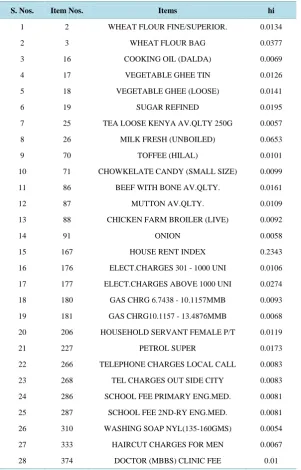
Table 1. Significant hat values for the items exceeding cut-off value 0.005348.

S. Nos. Item Nos. Items hi

1 2 WHEAT FLOUR FINE/SUPERIOR. 0.0134

2 3 WHEAT FLOUR BAG 0.0377

3 16 COOKING OIL (DALDA) 0.0069

4 17 VEGETABLE GHEE TIN 0.0126

5 18 VEGETABLE GHEE (LOOSE) 0.0141

6 19 SUGAR REFINED 0.0195

7 25 TEA LOOSE KENYA AV.QLTY 250G 0.0057

8 26 MILK FRESH (UNBOILED) 0.0653

9 70 TOFFEE (HILAL) 0.0101

10 71 CHOWKELATE CANDY (SMALL SIZE) 0.0099

11 86 BEEF WITH BONE AV.QLTY. 0.0161

12 87 MUTTON AV.QLTY. 0.0109

13 88 CHICKEN FARM BROILER (LIVE) 0.0092

14 91 ONION 0.0058

15 167 HOUSE RENT INDEX 0.2343

16 176 ELECT.CHARGES 301 - 1000 UNI 0.0106

17 177 ELECT.CHARGES ABOVE 1000 UNI 0.0274

18 180 GAS CHRG 6.7438 - 10.1157MMB 0.0093

19 181 GAS CHRG10.1157 - 13.4876MMB 0.0068

20 206 HOUSEHOLD SERVANT FEMALE P/T 0.0119

21 227 PETROL SUPER 0.0173

22 266 TELEPHONE CHARGES LOCAL CALL 0.0083

23 268 TEL CHARGES OUT SIDE CITY 0.0083

24 286 SCHOOL FEE PRIMARY ENG.MED. 0.0081

25 287 SCHOOL FEE 2ND-RY ENG.MED. 0.0081

26 310 WASHING SOAP NYL(135-160GMS) 0.0054

27 333 HAIRCUT CHARGES FOR MEN 0.0067

28 374 DOCTOR (MBBS) CLINIC FEE 0.01

0 0.5 1 1.5 2 2.5 3 3.5 4 4.5

x 104 -1

-0.5 0 0.5 1

Observations

R

es

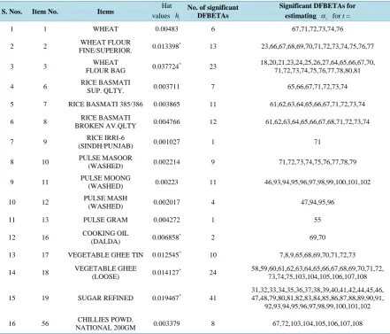
[image:5.595.149.451.247.718.2]

(6)

[image:6.595.148.485.182.296.2]

Table 2 presents list of items with the significant DFBETAs exceeding the cutoff value 0.00995. The large values of hi are represented by the values with superscript

*

. Out of these 37 influential items, 32 are from the first commodity group food and beverages that include wheat flour, vegetable ghee, sugar, beef with bones, and mutton with the corresponding higher diagonal values of hat matrix. Sugar refined with h19=0.019467 has an impact on estimation index number relating to 41 months or in other words, it affects the values of 41 alphas in parameter vector β. Other influential commodity groups include house rent with the highest h167=0.234298, fuel and lighting, and transportation and communication.

[image:6.595.91.533.338.715.2]

Figure 2. Divisia index numbers including all items, excluding house rent and wheat flour.

Table 2. Significant DFBETAs corresponding to items and their hat values.

S. Nos. Item No. Items Hat

values hi

No. of significant DFBETAs

Significant DFBETAs for estimating αt for t =

1 1 WHEAT 0.00483 6 67,71,72,73,74,76

2 2 WHEAT FLOUR

FINE/SUPERIOR. 0.013398

* ₁₃ _{23,66,67,68,69,70,71,72,73,74,75,76,77}

3 3 WHEAT

FLOUR BAG 0.037724

* ₂₃ 18,20,21,23,24,25,26,27,64,65,66,67,70,

71,72,73,74,75,76,77,78,80,81

4 6 RICE BASMATI

SUP. QLTY. 0.003711 7 65,66,67,71,72,73,74

5 7 RICE BASMATI 385/386 0.003865 11 61,62,63,64,65,66,67,71,72,73,74

6 8 RICE BASMATI

BROKEN AV.QLTY 0.004766 12 61,62,63,64,65,66,67,68,71,72,73,74

7 9 RICE IRRI-6

(SINDH/PUNJAB) 0.001027 1 71

8 10 PULSE MASOOR

(WASHED) 0.002214 9 71,72,73,74,75,76,77,78,79

9 11 PULSE MOONG

(WASHED) 0.00223 11 46,93,94,95,96,97,98,99,100,101,102

10 12 PULSE MASH

(WASHED) 0.002017 4 47,94,95,96

11 13 PULSE GRAM 0.004272 1 55

12 16 COOKING OIL _(DALDA) 0.006858* 2 69,70

13 17 VEGETABLE GHEE TIN 0.012545* ₁₀ _{7,8,9,65,68,69,70,71,72,73}

14 18 VEGETABLE GHEE

(LOOSE) 0.014127

* ₂₄ 58,59,60,61,62,63,64,65,66,67,68,69,70,71,72,

73,74,75,103,104,105,106,107,108

15 19 SUGAR REFINED 0.019467* ₄₁ 31,32,33,34,35,36,37,38,39,40,41,42,44,45,46, _{47,48,79,80,81,82,83,84,85,86,87,88,89,90,91,}

92,93,94,95,96,97,98,99,100,101,102

16 56 CHILLIES POWD.

NATIONAL 200GM 0.003379 8 67,72,103,104,105,106,107,108

0 20 40 60 80 100 120

0 2 4 6 8 10

Tim Periods

D

iv

is

ia I

ndex

N

um

ber

s

(7)

Continued

17 71 CHOWKELATE CANDY

(SMALL SIZE) 0.009914

* ₁₂ _{13,14,15,16,17,18,19,20,21,22,23,24}

18 86 BEEF WITH BONE

AV.QLTY. 0.016098

* ₅ _{22,26,27,28,29}

19 87 MUTTON AV.QLTY. 0.010883* ₂ _22,23

20 88 CHICKEN FARM

BROILER (LIVE) 0.009158

* ₅ _{11,16,32,57,58}

21 89 EGGS FARM 0.004119 3 32,57,91

22 90 POTATOES 0.005345 15 23,24,26,27,28,29,30,31,32,33,34,35,36,45,78

23 91 ONION 0.005776* ₃₁ 1,2,3,4,18,19,20,21,24,25,26,27,28,33,34,35,53,54,

55,55,56,57,63,80,81,82,82,83,99,100,101,102,103

24 94 TOMATOES 0.004372 28 16,17,18,27,31,32,33,35,49,50,51,52,54,59,60,64,

67,68,69,84,85,87,98,99,102,103,104,104,105

25 101 PEAS 0.001467 3 16,42,43

26 107 CHILLIES GREEN 0.001443 3 19,69,104

27 108 CARROT 0.000802 1 4

28 109 GINGER 0.0013 9 21,22,23,24,25,26,27,28,29

29 110 GARLIC 0.001363 13 86,87,88,89,90,91,92,93,94,95,96,97,98

30 113 KINNU 0.001372 11 11,49,50,51,52,53,56,57,58,59,60

31 114 APPLE 0.004015 1 37

32 119 MANGO KALMI 0.00224 1 50

33 167 HOUSE RENT INDEX 0.234298* ₇ _{30,84,85,86,87,88,89}

34 177 ELECT.CHARGES

ABOVE 1000 UNI 0.027371

*

5 85,86,87,88,102

35 227 PETROL SUPER 0.017253* ₁₅ _{33,36,37,38,39,40,41,42,43,44,45,46,47,73,74,75}

36 266 TELEPHONE CHARGES

LOCAL CALL 0.00828

* ₁₂ _{94,95,96,97,98,99,100,101,102,103,104,105}

37 268 TEL CHARGES OUT

SIDE CITY 0.00828

* ₁₂ _{94,95,96,97,98,99,100,101,102,103,104,105}

5. Conclusion

In this paper, we use the general expression of hat matrix and DFBETA measure to detect the influential observations in order to estimate the Divisia price index number when the error is generated from AR(1) process. The hat values only depend on the weights of commodities, showing that the corresponding weights of consumer items have large influence on the parameter estimates and are not affected by the parameter of autoregressive process AR(1). An example is presented with reference to price data of Pakistan. From the findings of both hat matrix and DFBETAs, food and beverages are the leading commodity group as the maximum number of items in which group has large hat values and DFBETAs measures.

Acknowledgements

The authors are thankful to Dept. of Computer Science and Dept. of Statistics University of Karachi for provid- ing computing and research facilities and Dr Ejaz Ahmed, Dean CCSIS ,Institute of Business Management Ka- rachi for technical discussion and support.

References

(8)

Stat. No. 383, University of Chicago.

[2] Kadiyala, K.R. (1968) A Transformation Used to Circumvent the Problem of Autocorrelation. Econometrica, 36, 93-96.

http://dx.doi.org/10.2307/1909605

[3] Griliches, Z. and Rao, P. (1969) Small-Sample Properties of Several Two-Stage Regression Methods in the Context of Autocorrelated Disturbances. Journal of American Statistical Association, 64, 253-272.

http://dx.doi.org/10.1080/01621459.1969.10500968

[4] Maeshiro, A. (1979) On the Retention of the First Observation in Serial Correlation Adjustment of Regression Models.

International Economic Review, 20, 259-265. http://dx.doi.org/10.2307/2526430

[5] Park, R.E. and Mitchell, B.M. (1980) Estimating the Autocorrelated Error Model with Trended Data. Journal of Econometrics, 13, 185-201. http://dx.doi.org/10.1016/0304-4076(80)90014-7

[6] Belsley, P.A., Kuh, E. and Welsch, R.E. (1980) Regression Diagnostics. John Wiley, New York.

http://dx.doi.org/10.1002/0471725153

[7] Cook, R.D. (1977) Detection of Influential Observations in Linear Regression. Technometrics, 19, 15-18.

http://dx.doi.org/10.2307/1268249

[8] Cook, R.D. (1979) Influential Observations in Linear Regression. Journal of American Statistical Association, 74, 169- 174. http://dx.doi.org/10.1080/01621459.1979.10481634

[9] Cook, R.D. and Weisberg, S. (1982) Residuals and Influence in Regression. Chapman and Hall, New York.

[10] Draper, N.R. and John, J.A. (1981) Influential Observations and Outliers in Regression. Technometrics, 23, 21-26.

http://dx.doi.org/10.1080/00401706.1981.10486232

[11] Draper, N.R. and Smith, H. (1998) Applied Regression Analysis. 3rd Edition, John Wiley, New York.

[12] Puterman, M.L. (1988) Leverage and Influence in Autocorrelated Regression Model. Journal of the Royal Statistical Society, 37, 76-86.

[13] Cochrane, D. and Orcutt, G.H. (1949) Application of Least Squares Regression to Relationships Containing Autocor-related Error Terms. Journal of American Statistical Association, 44, 32-61.

[14] Stemann, D. and Trenkler, G. (1993) Leverages and Cochrane-Orcutt Estimation in Linear Regression. Communication in Statistics-Theory and Methods, 22, 1315-1333. http://dx.doi.org/10.1080/03610929308831088

[15] Barry, A.M., Burney, S.M.A. and Bhatti, M.I. (1997) Optimum Influence of Initial Observatins in regression Models with AR (2) Errors. Applied Mathematics and Computations, 82, 57-65.

http://dx.doi.org/10.1016/S0096-3003(96)00024-0

[16] Judge, G.G., Griffiths, W.E., Hill, R.C., Lutkepohl, H. and Lee, T.C. (1985) The Theory and Practice of Econometrics. 2nd Edition, John Wiley, New York.