A Biologically Inspired Clustering Algorithm Dependent on Spatial Data in Sensor Networks

Abstract— Sensor networks in environmental monitoring applications aim to provide scientists with a useful spatio-temporal representation of the observed phenomena. This helps to deepen their understanding of the environmental signals that cover large geographic areas. In this paper, the spatial aspect of this data handling requirement is met by creating clusters in a sensor network based on the rate of change of an oceanographic signal with respect to space. Inspiration was drawn from quorum sensing, a biological process that is carried out within communities of bacterial cells. In this system, global behaviour emerges from small-scale local events and this is an ideal characteristic of sensor networks. A spatial data model that showed the variation of water height as waves flow from the sea to the shore was used with real temporal data to test the algorithm. The paper demonstrates the control the user has over the sensitivity of the algorithm to the data variation and the energy consumption of the nodes while they run the algorithm.

Index Terms— biological algorithms, clustering, spatial data dependency, sensor networks

I. INTRODUCTION

LUSTERING is a useful technique to adopt in sensor networks when collecting the data measured at a central base station. As opposd to communicating directly with the base station, the nodes can form clusters to facilitate the aggregation of their data into representations collected in that area. This approach is energy efficient due to the fact that the sensor nodes are prevented from using a lot of energy to transmit their data over large distances. Forming clusters of sensor nodes has the additional advantage of robustness to device failure caused by hostile environments and energy depletion [1]. The clusters reduce the data dependency on individual nodes by encouraging collaboration between sensor nodes and by distributing the work load amongst the members of the clusters as fairly as possible.

Realising these benefits of clustering involves deciding

Manuscript received September 13th _{2004. A project of the Envisens virtual} centre of excellence, part of the NextWave initiave, funded by the UK Department of Trade and Industry (DTI).

I. Wokoma is at University College London, London, WC1E7JE UK (phone: +44-20-7679-7605; e-mail: [email protected]).

the number of clusters the nodes must be divided into, a question that has been tackled by wide variety of research efforts in different applications [20]. This paper is concerned with the development of an algorithm that attempts to solve the problem in two ways. Firstly, the algorithm establishes the spatial variation of certain parameters extracted from the data collected. The clustering algorithm is applied to the Self-Organising Collegiate Sensor Network (SECOAS), [2] a project which involves the continuous collection of oceanographic data from a sensor network placed on a sand bank to monitor the coastal effects of wind-farming. Secondly, the algorithm incorporates concepts from self-organising biological systems that use distributed mechanisms amongst low level entities to achieve a global goal. The algorithm was inspired mostly by quorum sensing (QS), a biological process used by bacterial cells to monitor when the cell density in their vicinity exceeds a certain threshold causing a change in their behaviour. The development of the algorithm was combined with previous work on the firefly/gossip protocol since this provided a good communication mechanism for the sensor nodes [3]. The parameters from the SECOAS data collected serve as a guide for the cluster formation, while the biological concepts allowed the clusters to be formed in a distributed fashion. The overall outcome is the emergence of clusters from the network without any user pre-determination or central management.

II. BACKGROUND

A. Parameter Extraction from SECOAS data

The key objective of the SECOAS project is to prove that a network of self-organising microcontrollers can be used by environmental scientists to tackle challenging sensing and monitoring applications. The sensor network needs to provide raw data containing oceanographic measurements of physical quantities such as pressure, tilts, temperature, sediment concentration and conductivity. In addition to producing this raw data, the

A Biologically-Inspired Clustering Algorithm

Dependent on Spatial Data in Sensor Networks

Ibiso Wokoma, Lam Ling Shum, Lionel Sacks, Ian Marshall

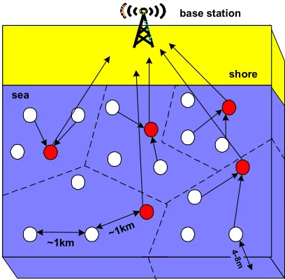
data handling techniques used in the project need to allow the nodes to carry out the processing needed to yield useful information from the data that may give the users a better understanding of the environment [4]. Currently, costly and immobile sea-bed landers that reside in one location for long periods of time are used in oceanographic monitoring but these are unable to provide the type of spatial and temporal information that coastal scientists are looking for. Sensor networks can overcome these disadvantages through the deployment of many inexpensive sensor nodes that are each given limited memory, power and communication abilities. The sensor nodes can then be operated with distributed algorithms that encourage collaboration between nodes and give the network the autonomy to respond to different environmental and technical events. These algorithms are supported on each node by an operating system called kOS, a lightweight and stateless system [25]. The QS algorithm is one of these algorithms designed to split the sensor network in SECOAS into clusters in a similar way to the diagram shown in Figure 1.

~1km

4-_8m

shore sea

base station

~1km

Figure 1: A model of the clustering in SECOAS; the cluster-heads are shown by the darker circles that forward data to the base station. All nodes are 1km apart and placed on the water surface 4-8m high.

An example of the data that the sensors will be collecting can be taken from WaveNet [5], a project that collects real-time wave data from areas at risk from flooding. One of these areas is at Scroby Sands in Great Yarmouth which is the planned location for the SECOAS trials. The data was collected in three locations in that area between April and June 2003 and taken in bursts of 1024 samples at 1Hz every hour to ensure that a wide spectrum of frequencies was observed [6]. A parameter

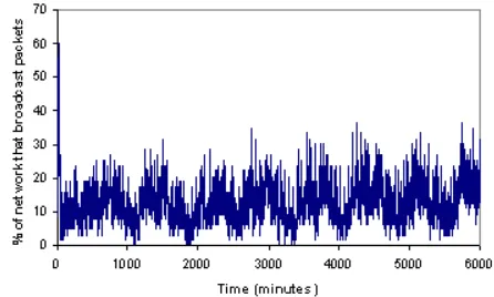
called the Physical Phenomenon of Interest (PPI) can be extracted from the raw data by a node-level compression agent being developed in SECOAS [2]. The PPI is a metric that can correspond to any one of a broad range of physical quantities in the environment at a specific time and can be used by the QS algorithm to give a useful meaning to the clusters. In this paper, the PPI represents the mean value of pressure per hour, which is proportional to the wave height measured by a node [7].The temporal variation of this PPI over a period of 100 hours extracted from the WaveNet data is shown in Figure 2 and used for simulations in Section V.

Figure 2: The PPI extracted from the WaveNet data; in this case it is the mean pressure per hour

B. Spatial Clustering

Cluster analysis is a branch of data mining or knowledge discovery in databases (KDD) which involves discovering patterns and interesting knowledge that may be hidden in data [8]. The application of data mining to spatial databases is relevant to the subject of this paper [9], since these types of databases can be used to represent the information collected from a sensor network. If classical statistical analysis were applied, the spatial attributes would be regarded as a complication and as a result would be discarded, but in this scenario the data collected has a high degree of spatial dependence and requires spatial variables to explain or predict the phenomenon under investigation [10]. Spatial data analysis is more appropriate since the objects can be stored in the database with topological/distance information as shown by the matrix Z, where z1- zk refers to one of k variables or attributes at the location s at the same sensor. The assumption is that the data values refer to the same point in time making it possible to suppress t

in the following equation [11]:

n i k i t s i t

z t i z t i z

Z = { ₁(, ), ₂(, ),..., ( , ) (), }_=1,...,

take one of several forms such as clusters. Spatial clustering forms groups between data objects with a high degree of spatial similarity between each other, in comparison to objects in other clusters. If spatial clustering is applied to a database to extract patterns from the data collected in a sensor network then the same technique could be used during the operation of the sensor network. For example, Figure 3 shows the sensor nodes in two regions around the centre of the network observing large spatial changes in the environmental signal compared to the rest of the network. In SECOAS, the remote user has the option of sending policies into the network that instruct the sensor nodes to change their behaviour; in this case the user may want the clusters in the two central regions to sample more frequently. The increase in the amount of data collected from those regions may help the user further their understanding of the signal activity in that area. One way of making this scenario possible is to form clusters based on finding spatial similarity in the change of signal on-the-fly.

environmental signal

sensor network

Distance

Figure 3: A sensor network observing an environmental signal and forming clusters in areas of similar gradient. Sensor nodes with the same pattern belong to the same cluster. Smaller clusters form around the centre due to the large changes in the signal.

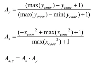
The development of the QS algorithm required experimentation with test data that showed not only the temporal data in Figure 2 but also the concurrent spatial variation at multiple locations to fully represent the data that a sensor network will have to handle. As a result, the temporal data from Figure 2 was applied to a wave model constructed on the assumption that the wave height decreases from the sea to the shore as the tide comes in [12]. The height profile is divided into four components:

xcor, ycor, t and noise. xcor and ycor are arbitrary, the t component is derived from the real data and Xt is the time series. The following equations were used to generate the

spatial data:

(max( ) 1)

(max( ) min( ) 1) coor coor y

coor coor

y y

A

y y

− +

=

− +

2 2

2

( max( ) 1)

max( ) 1 coor coor x

coor

x x

A

x

− + +

=

+

,

x y x y

A =A A⋅

The temporal and noise aspect of the data were

incorporated into the model to produce the tempo-spatial model using the following equations

for every time step,

( ) min( ( )) max( ( )) min( ( ))

t t

t

t t

stat X stat X

A

stat X stat X

− =

−

, ,

x y t x y t

A =A A A⋅ ⋅

, , (0,1) * comb x y t

A =A +noise SNR

( )

comb t

A A= +mean X

Figure 4 gives a pictorial representation of this spatial variation. The QS algorithm assesses the change in the PPI over space by calculating the gradient of the observed signal between nodes.

Figure 4: (a) the spatial components and (b) the spatial components with temporal data and noise

C. Biological Concepts

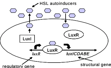
surrounding areas of the organ and build up in concentration. Autoinducers allow the cells to introduce themselves to each other and to determine if there are other cells present in the environment. As the concentration of Vibrio fisceri increases, the autoinducer accumulates to a threshold value of around 10µg/ml which allows the transcription of the luminescent proteins a necessary action for light production. Figure 5 gives a pictorial view of the process.

LuxI LuxR

LuxR

luxICDABE luxR

HSL autoinducers

structural gene regulatory gene

LuxI LuxR

LuxR

luxICDABE luxR

LuxI LuxRLuxR

LuxR LuxR

luxICDABE luxR

HSL autoinducers

structural gene regulatory gene

Figure 5: A bacterial cell transmits autoinducers from the Lux I gene and receives autoinducers when their

concentration exceeds a threshold. Lux R combines with the autoinducer to produce more Lux I, the proteins for bioluminescence – positive feedback.

In this context, a quorum is the minimum population of bacterial cells required to perform light production. The cells sense when they have a quorum by measuring the autoinducer concentration with their response regulators. This is applicable to the clustering process in SECOAS where the sensor nodes, like bacterial cells, are simple agents that interact on a local scale and cause global patterns to emerge, a common attribute of complex systems [15]. In a similar way to bacterial cells using quorum sensing, the sensor nodes need to determine when there are enough of them to form a cluster that monitors a change in the observed signal. Hence, the concepts of the process of quorum sensing were incorporated in the design of the QS algorithm. This, in conjunction with a variation of gossip called the firefly-gossip protocol [3], provides a way of encouraging peer-to-peer communication and the self-organization of the network around spatial attributes.

III. RELATED WORK

Clustering can be separated into partitioning, hierarchy, density-based, and grid-based methods [16] and is usually treated as a centralized problem. However, this is not a valid approach for sensor networks since the nodes make their own decisions about the clusters they

want to be a part of, a similar situation to other large multi-agent systems [17]. The iterative process of the QS algorithm makes it similar to other partitioning clustering methods nodes. The difference is that the nodes do not make use of a cost function to decide on the best clustering and instead update their measurements of the environment. The algorithm operates in a decentralized fashion, thus making the sensor network work like the biological processes discussed. No limits are placed on the algorithm concerning the cluster size like other partitioning algorithms thus allowing the formation of clusters of arbitary shape that are possibly more representative of the selected features in the data.

• Each node has at least one clusterhead as a neighbour

• Each node joins the cluster of a neighbouring clusterhead with the highest weight

• Two clusterheads cannot be side-by-side

The way the weights are allocated are left up to the user thus for the purpose of the comparison in Section V, the weights were given values that were data dependent rather than mobility dependent.

IV. THE QS ALGORITHM

A. Algorithm Details 1) Assumptions

The QS algorithm [22] makes the following assumptions about the nodes in a sensor network:

• They spend most of the time asleep and wake up periodically to transmit packets to their neighbours and to forward data to the base station. They also have control over their variable duty cycle.

• They must be deployed in such a way that they have at least one neighbour and no two nodes occupy the same position.

• They are quasi-stationary, have a fixed transmission radius and can communicate with any neighbour within that radius.

• They are location aware as they are supplied with co-ordinates from the auto-location algorithm that runs concurrently on the nodes [23].

• They are identical and have equal capabilities with no awareness of global scale event

2) Measuring the Signal Spatial Changes

The algorithm aims to allow the network to establish clusters based on the spatial changes in the observed signal by measuring the gradient of the signal between nodes. If the gradient of the observed phenomena does not stay constant over the whole area then the nodes have to decide how to group the gradients measured. This is measured with a parameter called the gradient range and, like the gradients, is measured in signal units per unit distance. At first, the nodes have different ideas about what this gradient range of a cluster should be since they initialize this parameter with the minimum difference between any pair of gradients measured between them and their neighbours. During the execution of the algorithm, the nodes converge to a common, or if not similar, value for the gradient range through averaging so that when the clusters eventually do form the nodes can calculate boundaries of gradients allowed in a cluster

without having to consult a cluster-head. Thus, the nodes can work in a fully distributed manner by deciding for themselves which neighbours can join their cluster and the boundaries can prevent an overlap in spatial changes observed by the clusters.

For example, if a network reaches a decision to set the gradient range to 10 signal units per unit distance then the clusters will be formed every time the gradient of spatially varying environmental signal changes by 10 signal units per unit distance. If a node is in a cluster has this gradient range and monitors gradient changes between 20 and 30 signal units per unit distance then it will only leave the cluster to join another or to reset and become ungrouped if the gradients measured with any of its cluster neighbours does not fall within those boundaries.

3) Algorithm Control Packets

The nodes can transmit and receive two types of packet. The first is the Node Synchronization (NS) packet which is used to transmit information between nodes concerning their identification number and sample measurement. These packets allow the nodes to calculate the gradient of the observed phenomena between them and each of their neighbours. The nodes store the gradients measured to allow them to determine the gradient range they think a cluster should have by finding the minimum difference between any pair of gradients. The packets also transfer the gradient ranges of surrounding neighbours. Once the nodes make a record of this, they can adjust their gradient range by taking the average of these values.

The second is the Group Synchronisation (GS) packet which is only transmitted alternately with the NS packets by potential clusterheads and cluster members. A node can determine whether it is a clusterhead by using the pair of gradients that gave the initial gradient range to calculate the boundaries of a cluster. If both those gradients fall within the boundaries then the node can form a cluster with the two neighbours that gave the gradients.

changes to the cluster parameters or any user policies between cluster members.

When NS and GS packets are passed between nodes of the same cluster during intra-cluster communication, they act like autoinducers by allowing the nodes to extend the period before their next broadcast. When the period reaches a maximum the nodes know they are in a quorum cluster, the minimum number of sensors required to monitor a particular change in the environmental signal and transmit the cluster information to the base station. Until a cluster has nodes that reach this quorum status, it is known as temporary cluster that may only exist due to changes in the environmental signal that do not last very long.

4) Packet Transmission and Reception

The frequency of packet transmission, which is carried out by allowing sensor nodes to broadcast information to their neighbours, is varied according to the algorithm which reflects the activity of the environmental signal. The adjustment of gradient range of the nodes, the resetting of a node due to the breakdown of a temporary or quorum cluster and the lack of contact that a cluster member receives from its cluster neighbours all result in the node broadcasting at a high rate. If the nodes end up in clusters then the broadcasting frequency will be reduced. The algorithm does not require all the nodes to be up-to-date. As the algorithm is iteratively executed, it eventually converges to the right solution

In SECOAS, the sensor network is likely to encounter storms where the amount of activity in the sea will prevent effective communication between the nodes. Sending and receiving NS and GS packets under these conditions will not be possible and since the environmental signal will be changing rapidly between the nodes, they would be unable to form clusters anyway. In this case, it would be more beneficial for the nodes to log data and forward them to the base station at a more convenient time

B. Algorithm Pseudocode

A sensor network can be modelled as a collection of N

sensor nodes at points within a set of vertices called V, where V = {v1, v2…vN }. The links that exist between the nodes can be represented by a set of edges labelled E, where E = {e1, e2…eN}. Initially, these links represent the communication channels between neighbouring sensor nodes and after the execution of the algorithm some these links will chosen to represent the connections within any clusters that are formed. The vertices can be identified

with a unique id or by the co-ordinates [x, y], while the edges are defined by their endpoints (u, z) where u and z

are both members of V. Hence, the complete network can be represented by the graph G = (V, E) which after the execution of the QS algorithm will lead to the formation of a new graph G’ = (V, E’) where the nodes connected by links in E will represent clusters of V.

The following representations also apply to this model:

• S = {s1, s2…sN } is the data matrix of the nodes in V represented by a set of sample measurements made by the nodes.

• M = {mu1, mu2…muN”} is the set of gradients formed between sensor node u and each of the neighbours, where u

∈

• ru is the gradient range of sensor node u and r = {r1,

r2…rN”}is the gradient ranges of the neighbours of u.

• BLu and BHu are the lower and higher boundaries of gradients allowed in a cluster respectively.

• CPu shows whether u can become a cluster-head

• tb is the period before the next broadcast of u and tbmax to the maximum value allowed for tb.

Given these symbols, the algorithm pseudocode is shown below:

I. INITIALIZATION

ru = CPu = 0, Cu = BLu = BHu = null,

r = M = {}, tb = 5 epochs, tbmax = 60 epochs

II. ANALYSIS OF RECEIVED NS PACKETS for each received NS packet,

u calculates muz, the gradient between the itself and sender of the NS packet, z, which is duz distance

units away using:

uz z u uv

d s s

m = − . This is stored in

set M; u also deletes entries in M that have not been updated for a long time.

end for

III. GRADIENT RANGE ADJUSTMENT If N” > 2,

a. Let the standard deviation of r be

σ

coefficient of variation

<

0

.

05

r

r

σ

u =

rmax, the maximum value of r. Otherwise,

"

1

N

r

r

r

N

n n mean

u

∑

=

=

b. Set the smallest difference between any pair of

gradients in M using

[

]

[

]

1 " 1 min

min

u

r

m

m

r

= =

−

=

=

y < z.

c. The pair of gradients used to calculate rmin are

mh and ml where mh > ml. Let

∈

Ζ

r

m

Check whether the following condition is true:

















+













<

≤













*

*

r

r

r

m

m

r

r

m

d. If the condition is not satisfied, then repeat

rmin = 0.25 * rmin until it is.

IV. CLUSTER-HEAD PROPOSAL

Carry out step III, part (c) but substitute ru for rmin. If the condition is true, then u is a potential cluster-head.

Thus CPu = 1,

u l Lu

r

m

B

=

B

=

B

+

r

send out GS packets alternately with NS packets. V. ANALYSIS OF GS PACKETS

for each received GS packet,

- Cluster Formation and Expansion

Find muz, where muz is the gradient between sensor node u and the sender of the GS packet, z, from the set M.

if CPu = 0 or (CPu = 1 and BLu = BLz), BLz≤muz<

BHz and ru = rz,

u copies the cluster information (Cz, BLz, BHz) from the sender z

add link to E*

end if

- Intra-cluster Communication and Quorum Sensing if u and z are in the same cluster, i.e. Cu = Cz, and

ru = rz,

messages passed between cluster members and tb increasesd; if tb >= tbmax then u knows it is in a quorum

end if

- Inter-cluster communication

if u and z are in different clusters, i.e. Cu≠Cz, if BLu = BLz,

u copies the cluster information from the sender z

else,

messages can be passed between clusters endif

end if end for

VI. RESET

if the condition BLu≤mn < BHu not satisfied for all entries in M or there is little or no contact with other cluster members

u erases its’ cluster information and broadcasts only NS packets

remove link from E*

end if

V. PERFORMANCE EVALUATION

The algorithm was performed using Netlogo [26] on an evenly spaced grid of nodes that each observed the temporal data shown in Figure 2. This data was scaled according to the position of each node in the spatial model shown in Figure 4. The effects of varying the parameters of the algorithm were individually assessed in a network of 63 nodes by observing number of temporary clusters, the number of quorum clusters, the amount of communication between the nodes and the energy consumed by the network while running the algorithm.

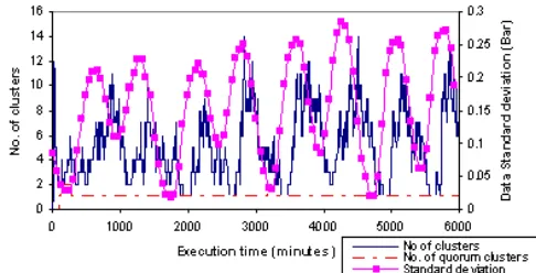
The QS algorithm reacts to changes in the observed phenomena by allowing nodes to update each other on any changes in their sample measurements that will invariably alter the gradient of the signal measured between them. The sensitivity of the algorithm to these environmental changes can be controlled by varying the number of broadcasts the nodes need to make before an carrying out an update. The graph in Figure 8 shows the algorithm with the highest sensitivity setting; the nodes continuously update the gradients every time there is a change in the sample measurement regardless of the number of broadcasts.

Figure 6: The number of clusters and data standard deviation over time

deviation of the samples of the environmental signal from all the nodes and the number of clusters formed by the sensor network measured each minute. The fast fourier transform was computed for both factors in Figure 8 to observe the frequency of the variation. The power spectrum indicated that the variation of both factors reached a maximum value every 750 minutes, thus the number of clusters formed varies at the same rate as the environmental signal. After the initialization of the algorithm, every time the standard deviation reached a maximum value, the number of clusters took around 180 minutes to respond by increasing to a maximum of 12 to 14 clusters. When the standard deviation was at its lowest value, all the nodes formed a single cluster.

The sensitivity of the algorithm was decreased by increasing the period before which a node would allow a neighbour to update the gradient. This period was measured by the number of broadcasts made by the node. Figure 9 shows the graph for the effect of this on the maximum number of clusters that represents the point where the standard deviation of the data by all the nodes is the largest is shown in Figure 9(a).

Figure 8 also shows that many of the temporary clusters formed do not exist long enough to accumulate NS and GS packets to form quorum clusters. It was stated in the previous section that the NS and GS packet exchange between the members of the same cluster result in the increase of the period before the node’s next broadcast, tb. Thus the sensitivity of the algorithm is not only indicated by the number of temporary clusters made but also the proportion of temporary clusters that become quorum clusters. Figure 9(b) shows how the increase in tb affects this proportion of quorum clusters to temporary clusters while keeping the number of broadcasts before a gradient update at a constant value of 1.

Figure 7: (a) The effect of the number of broadcasts of any node before a gradient update on the temporary and (b) the effect of the tb increase on the number of quorum

clusters

As the number of broadcasts before a gradient update

increases, the maximum number of clusters decreases showing that not every change in the observed phenomena results in the formation of a cluster. Only the changes that have an impact are those that occur when the nodes are ready to update the gradients. However, the oscillation of the number of clusters still occurs in a similar way to the variation in Figure 8. Figure 9 also shows that the increase in tb due to a NS/GS packet between cluster members is proportional to the percentage of temporary clusters that become quorum clusters. Large increases in tb make cluster members assume quorum cluster status quickly and since they broadcast less often they do not reset for a long time.

The user of the sensor network should be given control over how sensitive the algorithm is to the observed phenomena; if every change in the environment is to be observed then the number of broadcasts before a gradient update should be kept low and the tb increase should be kept high.

As stated in Section III, the QS algorithm is concerned with mining spatial patterns as efficiently as possible. It does this by modulating the activity of the sensor nodes with the changes they observed by of the environmental signal which is achieved by increasing or decreasing the period tb. This is demonstrated by the graph in Figure 10 where the increases in the number of broadcasts before a gradient update and the increases in tb due to a GS or NS packet are low.

Figure 8: The percentage of broadcasting nodes over time while the QS algorithm is executed; this indicates the amount of communication taking place in the network

Initially, the number of broadcasting nodes is high as the nodes are not in any clusters. As the algorithm proceeds, the percentage of the nodes sending out messages falls from 60% to 2% as the nodes settle into their clusters. The percentage of broadcasting nodes varies between 2% and 30% at the same rate as the data.

consumption of the network was observed by applying a simple energy model which has been used in the research of several clustering algorithms [18, 19, 20]. The assumptions in this model are concerned with the actions that expend energy such as the transmission and reception of each bit of data between sensors and that there is a continuous function for energy consumption. Assumptions were made about the values of εelec, the energy required to drive the transmitter/receiver circuitry, and εamp, the energy required for the transmitter amplifier during communication. An additional assumption was made about the energy required for data fusion when the clusters have been formed and the transmission of the aggregated data to the base station being the same as the transmission of data between sensors except over a longer distance. The parameters that are derived from these assumptions are listed in Table 1 and to validate their use with the QS algorithm, the scale of the network was altered to make it similar to the networks used in [18, 23]. Thus, the nodes in the network were evenly spaced by 1m apart instead of the 1km separation that will be used in the SECOAS trial and the following equations were used for calculating TXi,j, the energy expended when transmitting k bits of sensor data from sensor i to sensor j

which is di,j m away, and RXi, the energy spent on receiving k bits at sensor i:

(

)

k

RX

k

d

TX

elec j i

j i amp elec j

i

*

*

*

,

2 , ,

ε

ε

ε

=

+

=

Table 1: The parameters used for simulating energy dissipation

Parameter Value

εelec 50nJ/bit

εamp 100pJ/bit/m2 Initial energy 0.5J

Packet size 2000bits Fusion energy 5nJ/bit/message

The same parameters were used when running the DMAC algorithm stated in Section III under the same conditions for comparison to the QS algorithm. The DMAC algorithm requires that the nodes are allocated with weights, thus to make the algorithm dependent on the spatial data variation of the observed phenomena, the weights allocated were made equal to average of the gradients between each sensor node and their neighbours. The nodes that measure the largest gradient are observing

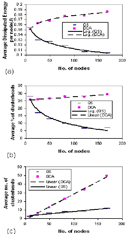
the biggest change in that area making them good cluster-heads in that region. The gradient dependent weights in the DMAC algorithm allow the nodes to react to spatial signal changes by continuously changing the clusterheads. This makes it suitable for the comparison to the QS algorithm which tries to do the same thing. The QS and DCA algorithm were executed on square sensor networks that were increased in size from 9 to 169 nodes. In each case, the cluster-heads select at random a node from their cluster to send aggregated data to a base station with the co-ordinates (-13, 0) after forming clusters. Figure 11 shows the average energy dissipated after 3000 epochs at each node, the average percentage of cluster-heads and the average number of clusterheads as the network size increases.

Figure 11(a) and (b) shows that when the network uses QS algorithm it consumes less energy as the number of nodes increase. This may be due to the fact that the decreasing proportion of cluster-heads. The opposite applies to the DCA algorithm; the amount of energy dissipated increases with network size as the number of cluster-heads also increases. The reason for this is the restriction of the DCA algorithm on the size of the clusters created; it requires that neighbours must be within a one-hop distance of a cluster-head. The QS algorithm, on the other hand, allows the cluster to be as large as is necessary to reflect the change in the environmental signal. As the network size increases, the number of clusters created with the QS algorithm increases only slightly as shown in Figure 11(c) which suggests those clusters become larger to contain more nodes that observe similar spatial changes. It also suggests for a range of networks of certain size approximately the same number of clusters will be created since this is all that is needed to represent the environmental signal. If the signal fluctuated more rapidly, then the QS algorithm would require more energy to form smaller clusters and would have more nodes communicating with the base station. The energy consumption depends on the signal variation which in this case as opposed to the number of nodes.

VI. CONCLUSIONS AND FUTURE WORK

The QS algorithm provides a method of clustering in sensor networks based on the spatial patterns in an environmental signal. The results show that the algorithm has two parameters that control the sensitivity of the clustering to the variation of the signal: the number of broadcasts before a gradient update and the tb increase due to NS/GS packets passed between cluster members. Although energy is not used as a guide to forming the clusters, energy savings are gained by reducing the communication between nodes when the clusters were formed. The QS algorithm formed less clusters than the DCA algorithms regardless of the network size because of the environmental signal. This also saved energy and allowed the algorithm to scale well with the increase in network size. Future work will involve the implementation of the algorithm on real sensor nodes in the SECOAS trials, an assessment of the effect of processing costs of the algorithm on the energy costs and the experimentation of the algorithm on other spatial signals.

REFERENCES

[1] D. Estrin, R. Govindan, J. Heidemann, S. Kumar, “Next century challenges: Scalable coordination in sensor networks”, In Mobile Computing and Networking, pp. 263--270, 1999. [2] L. Sacks, “The Development of a Robust, Autonomous Sensor

Network Platform for Environmental Monitoring”, Sensors & their Applications XII conference, Limerick, Sep. 2003. [3] I. Wokoma, I. Liabotis, O. Prnjat, L. Sacks, I. Marshall, “A

Weakly Adaptive Gossip Protocol for Application Level Active Networks, IEEE 3rd International Workshop on Policies for Distributed Systems and Networks, June 2002.

[4] L. Shum et al, “Distributed Algorithm Implementation and Interaction in Wireless Sensor Networks, Second International Workshop on Sensor and Actor Network Protocols and Applications, August 2004.

[5] Wavenet: http://www.cefas.co.uk/wavenet/.

[6] D. Ganesan, D. Estrin and J. Haidemann, “Dimension, why do we need a new data handling architecture for Sensor Network”, ACM SIGCOMM Computer Communication Review Volume 33 , Issue 1, January 2003.

[7] R. M. Sorensen, “Basic wave mechanics : for coastal and ocean engineers”, Wiley Interscience, 1993.

[8] W.J. Frawley et al, "Knowledge discovery in databases: an overview", Knowledge Discovery in Databases, pp. 1-27. AAAI Press, 1991.

[9] K. Koperski et al, “Spatial Data Mining: Progress and Challenges Survey Paper”, SIGMOD Workshop on Research Issues on Data Mining and Knowledge Discovery, Montreal, Canada, June 1996.

[10] J. Weeks, “Introduction to Spatial Analysis”, Poverty and Food Insecurity Mapping Case Studies Workshop, FAO HQ, Rome, Italy, 2002.

[11] R. Haining, “Spatial Data Analysis”, Cambridge University Press, 1st _{Edition, 2003.}

[12] Open University Course Team, “Waves, Tides and Shallow-Water Process, Second Edition”, Butterworth Heinemann, 1999.

[13] M. B. Miller, Bonnie L. Bassler, “Quorum Sensing in Bacteria”, Annual Review in Microbiology, pp.165-99, 2001. [14] M. E. Taga, B. L. Bassler, “Chemical communication among

bacteria”, Proceedings of the National Academy of Sciences of the USA, November 2003.

[15] S. Johnson, “Emergence: the connected lives of ants, brains, cities and software”, Allen Lane - The Penguin Press, 2001. [16] H. Miller, J. Han, “Spatial Clustering Methods in Data Mining:

A Survey”, Geographic Data Mining and Knowledge Discovery, Taylor and Francis, 2001.

[17] E. Ogston, B. Overeinder, M. van Steen, F. Brazier , “A Method for Decentralized Clustering in Large Multi-Agent Systems”, Second International Joint Conference on Autonomous Agents and Multi-Agent Systems, pp. 789-796, 2003.

[18] W. R. Heinzelmann, A. Chandrakasan, H. Balakrishnan, “Energy-efficient communication protocols for wireless microsensor networks”, in Proceedings of the Hawaii International Conference on System Sciences, January 2000. [19] S. Bandyopadhyay, E. J. Coyle, “An energy efficient hierchical

clustering algorithm for wireless sensor networks”, IEEE Infocom 2003.

[21] “Distributed clustering for ad hoc networks”, S. Basagni, Proc of Fourth International Symposium on Parallel Architectures, Algorithms, and Networks (I-SPAN), pp 310 – 5, June 1999. [22] I. Wokoma, L. Sacks and I. Marshall, “Clustering in Sensor

Networks using Quorum Sensing,” London Communications Symposium, University College London, 8th-9th September, 2003.

[23] T. Adebutu, L. Sacks and I. Marshall, “Simple position estimation for wireless sensor networks,” in the London Communications Symposium, University College London September, 2003

[24] K. Kalpakis, K Dasgupta, P. Namjoshi, “Efficient algorithms for maximum lifetime data gathering and aggregation in wireless sensor networks”. Computer Networks, Vol. 42(6), pp. 697-716, 2003.

[25] M.Britton, L.Sacks, “The SECOAS project: Development of a self organizing, wireless sensor network for environmental monitoring”, Second International Workshop on Sensor and Actor Network Protocols and Applications, August 2004. [26] U. Wilensky, NetLogo 1999,