Evaluating how predictable errors in expected income affect consumption

Munich Personal RePEc Archive

Evaluating how predictable errors in

expected income affect consumption

Giamboni, Luigi and Millemaci, Emanuele and Waldmann,

Robert

10 May 2007

Online at

https://mpra.ub.uni-muenchen.de/12939/

Evaluating how predictable errors in expected

income affect consumption

∗

Luigi Giamboni

Emanuele Millemaci

Robert J. Waldmann

May 10, 2007

Abstract

This paper studies whether anomalies in consumption can be explained by a be-havioral model in which agents make predictable errors in forecasting income. We use a micro-data set containing subjective expectations about future income. The paper shows that, the null hypothesis of rational expectations is rejected in favor of the be-havioral model, since consumption responds to predictable forecast errors. On average agents who we predict are too pessimistic increase consumption after the predictable positive income shock. On average agents who are too optimistic reduce consumption. (JEL classification: D11, D12, D84).

Key words: Behavioral Economics, Subjective Expectations, Rational Expectations, Consump-tion and Saving.

∗_{The authors thank Luigi Guiso and Tullio Jappelli for useful comments, as well as seminar participants}

at the University of Urbino. This research wouldn’t have been possible without the CentER at the University of Tilburg that supplied us with the data.

†_{CONSIP S.p.A.}

‡_{Facolt´a di Economia, Universit´a di Roma ”Tor Vergata”.}

§_{Facolt´a di Economia, Universit´a di Roma ”Tor Vergata”. Corresponding author. Tel.:}

1

Introduction

Under rational expectations the stochastic version of the permanent income hypothesis/life

cycle hypothesis (PIH/LCH) states that predictable changes in income should not help to explain the change in consumption. Under assumptions including the absence of liquidity

constraints, the change in consumption should depend only on innovations. We show that an apparent economic anomaly, predictable changes in consumption, may be explained

re-laxing the rationality hypothesis in favor of a behavioral model where agents are irrationally optimistic or pessimistic.

Since the path of future income is uncertain, the agent makes consumption decisions

based on his subjective expectation about future uncertain events. The PIH/LCH is our null hypothesis, the alternative is a behavioral model of consumption. In this second model

the agent aims to maximize his subjective expected utility over the life cycle, but he makes predictable (for the econometrician) systematic errors in forming subjective expectations on

future income. Hence, on average an individual who has been too pessimistic in making his prediction experiences a positive surprise when income is realized and is induced to revise his consumption decision upward. Conversely, if the agent has been overly optimistic he

experiences a negative shock on income and decides to lower consumption.

Our behavioral model implies a new formulation of the Euler equation where predictable

errors in income forecasts help explain the first difference of consumption. This suggests that, not properly taking into account irrationality, previous research on excess sensitiv-ity of consumption may be not correctly specified. We will show how the coefficient on

predictable changes in income changes once the predictable forecast error is introduced in the Euler equation. In particular, irrational pessimism and irrational optimism seem to be

more statistically significant explanations of the apparent anomaly in consumption than precautionary savings and liquidity constraints.

Despite the theoretical statement that actual actions depend on subjective expectations about future events, economists engaged in empirical research tend to be skeptical of the use of data on subjective expectations. The main practice has become that of inferring

expectations from realizations. The attempt to infer from the distribution of realizations requires the knowledge of the information set of the agent and how he uses it. Typically

the researcher imposes a model of the data generating process, which under the assumption of rational expectations describes how individuals form their expectations. The estimation

it one year into the future exploiting the orthogonality condition implied by the rational expectations hypothesis (see Hall and Mishkin, 1982).

In contrast direct elicitation of subjective expectations may eliminate the need for such assumptions, see Dominitz and Manski (1997), Flavin (1999) and Dominitz (1998, 2001).

It allows for complete heterogeneity of income expectations formation and permits one to overcome the problem that the econometrician’s information set is not rich enough to reproduce the agent’s information set.

Our data set consists of approximately 5000 individual observations for each wave in the Netherlands and contains detailed information on wealth, income, work and demographic

characteristics and different kind of subjective expectations stated by the respondents, covering the period that goes from 1993 to 2006.

We calculate the forecasts errors as the difference between realized family income and

the mean of the subjective distribution of its predictions. We instrument the agent’s pre-diction error with various specifications of the information set. The weak exogeneity of the

adopted instrument is assured by the null hypotheses of agents’ rationality. In the second step of the two stage instrumental variable estimator we regress the first difference of the

logarithm of consumption on the fitted (hence predictable) error and find strong evidence in support of our behavioral model stating that consumption responds to predictable errors in income forecasts.

It is often argued that works on the predictability of forecast errors, either rejecting or accepting the rational expectations hypothesis, do not supply evidence to support the

claim that the elicited expectations really correspond to those affecting the agent’s behav-ior. Hence, it is important and interesting to show that, once the rational expectations

hypotheses is rejected, it is possible to explain agents consumption decisions.

Section 2 contains our theoretical model. Section 3 describes our data set, with a particular focus on stated subjective expectations and realizations. In the same section,

we also describe the way we estimate consumption starting from self-reported income and savings data. Section 4 describes the empirical version of the models and discusses the

estimation strategy. Section 5 contains our empirical evidence that support the behavioral model versus the rational one, and the test on its out of sample predictive performance. Section 6 performs excess sensitivity test of consumption in our modified version of the Euler

equation. We show that irrationality is a statistically significant explanation, alternative and compatible with precautionary saving and liquidity constraints. We argue that previous

because of the assumption of rational expectations. Section 7 concludes.

2

The model

The path of future income is uncertain, so individuals must make their consumption plans on the basis of their subjective expectations about future uncertain events. The

conven-tional model of life-cycle consumption under uncertainty, with isoelastic time separable utility, consumers maximizing expected utility function and perfect credit markets,

be-comes:

M axc1,...,cTE su t [

∞

X

s=0

(1 +δ)−s c

1−γ t+s

1−γ|Ωt] (1)

subject to

at+s+1 = (1 +r)(at+s+yt+s−ct+s) s= 0,1, ...,∞ (2)

at given (3)

lims→∞(1 +r) −s

as= 0 (4)

where E_tsu is the subjective expectations operator conditional on all information available at time t, indicated with Ωt, and stated at the end of the period, δ is the intertemporal rate of time preference, c is consumption, y is total family net income, r is the real rate of interest, which is assumed to be constant, and a represents assets apart from human capital.

Differentiating with respect to consumption and considering the first order condition of equality of wealth’s and consumption’s marginal utilities at the optimum, we obtain the

following Euler equation:

E_tsu(c−γ t+1) =

1 +δ

1 +rc

−γ

t (5)

Assume that agents have a subjective distribution over the consumption growth rate, which

is normal:

∆ logct+1|Ωt∼N(µc;σ2c) (6)

where µc = Etsu(∆ logct+1) and σc2 = V arsut (∆ logct+1), that, for the sake of simplicity,

will be assumed constant over time. We also assume that e((1+γ)/2)σ2c+(˜r−δ˜)/γ

<1 +r and that the law of iterated expectations applies to subjective expectations,Esu

t (Etsu+s(xt+s)) =

and that they will be rational in the future. We can write down Eq. 5 as the following:

E_tsuexp[−γ∆ logct+1+ log(1 +r)−log(1 +δ)] = 1 (7)

which, in turn, is equal to

exp[−γµc+ (1/2)γ2σc2+ ˜r−δ˜] = 1 (8)

where we have exploited the property that if x∼N(µ;σ), than E(ex) =exp[µ+ (1/2)σ2], and to save on notation we have defined ˜r∼= log(1 +r) and ˜δ ∼= log(1 +δ). Taking the logs we have

−γE_tsu(∆ logct+1) + (1/2)γ2σc2+ ˜r−˜δ= 0 (9)

Splitting the logarithm and taking the exponential of both sides of the equation we are left with:

E_tsu(ct+1) =cte((1+γ)/2)σ

2

c+(˜r−δ˜)/γ

(10)

where we have again used the property of exponentials of normally distributed variables. Given the subjective expectations about future income held in period t, the individual’s perceived budget constraint can be expressed as:

∞

X

s=0

(1 +r)−s

Esu_t (ct+s) =at+ ∞

X

s=0

(1 +r)−s

E_tsu(yt+s) (11)

where yt is labor income which is exogenous and is paid at the end of the period. Substi-tuting in Eq. 10 gives

∞

X

s=0

(1 +r)−s

es[((1+γ)/2)σc2+(˜r−˜δ)/γ]

ct=at+ ∞

X

s=0

(1 +r)−s

E_tsu(yt+s) (12)

Using the assumption thate((1+γ)/2)σc2+(˜r−˜δ)/γ

<1 +r, we obtain

ct=ζ[at+ ∞

X

s=0

(1 +r)−s

where we have defined ζ = 1−e((1+γ)/₍₁₊2)σ2c_r+(˜₎r−δ˜)/γ. Moreover,at+1 is known at time t, so

ct+1−Etsu(ct+1) =ζ

∞

X

s=0

(1 +r)−s

[E_tsu₊₁(yt+s+1)−Etsu(yt+s+1)] (14)

The assumption that consumption is log normally distributed implies that

∆ logct+1 = (1/2)γσ2c + ˜

r−δ˜ γ +

+ ζ

Esu t (ct+1)

∞

X

s=0

(1 +r)−s

[E_tsu₊₁(yt+s+1)−Etsu(yt+s+1)]

(15)

Expectations are stated at the end of the period so E_tsu₊₁(yt+1) =yt+1. If one assumes

that the error in subjective forecasts ofyt+1,yt+1−Etsu(yt+1), is uncorrelated with

subjec-tive expectations of subsequent periods, i.e. E_tsu₊₁(yt+s+1)−Etsu(yt+s+1) = 0 fors >0, the

previous equation becomes:

∆ logct+1 = (1/2)γσc2+ ˜

r−˜δ γ +

ζ Esu

t (ct+1)

[yt+1−Etsu(yt+1)] (16)

If agents have been too pessimistic, i.e. yt+1 > Etsu(yt+1), they revise their

con-sumption decision upward. If they have been too optimistic, they revise their consump-tion decision down. More generally, if current forecast error is non negatively correlated

with the subjective expectations of subsequent periods, E_tsu₊₁(yt+s+1) −Etsu(yt+s+1) =

ρs[E_tsu₊₁(yt+1)−Etsu(yt+1)] andρ >0, we get to the following equation:

∆ logct+1= (1/2)γσc2+ ˜

r−δ˜ γ +

1 +r

1 +r−ρ

ζ[yt+1−Etsu(yt+1)

Esu t (ct+1)

(17)

That is the case if the agents believe that income innovations are persistent. If ρ= 1, agents believe that the unpredicted disturbance to yt is a random walk withEtsu(yt+s+1−

yt+s) = 0. Alternatively, if ρ= 1 and agents believe that the unpredicted disturbance toyt is an integrated moving average of the first order (IMA(1)) with MA coefficient equal to−θ, we have that Esu

t (yt+s+2−yt+s) = 0 fors≥0 andEtsu(yt+2−yt+1) =θ[yt+1−Etsu(yt+1)].

the shock will persist in the future. In this case Eq. 15 becomes:

∆ logct+1 = (1/2)γσc2+ ˜

r−δ˜ γ +

ζ(1 +r+θ)

r

[yt+1−Etsu(yt+1)]

Esu t (ct+1)

(18)

Asζ is less than ₁₊r_r and yt−1 > E_tsu(ct+1), forθ= 1 the coefficient of the forecast error is around 2.

Our model has the desirable feature of presenting consumption growth rate and con-sumption variation as the result of a precautionary saving motive plus a term that depends

on agents’ forecast errors. The second term is consistent with the idea of a behavioral model of consumption of irrationally optimistic agents who, stating larger expectations, experience a bitter surprise once income is realized and revise their consumption decision

downward. Conversely, irrationally pessimistic agents experience a positive shock as income is realized and revise their consumption decisions upward.

If agents were rational, E_tsu(yt+1) = Et(yt+1|Ωt) = yt+1, the model would state the

common result for a model without liquidity constraints that excess sensitivity is due to

precautionary saving, ∆ logct+1= (1/2)γσ2c+˜r −δ˜

γ . In this case, ignoring the variance term may result in omitted variable bias. Hence, overreaction of consumption to predictable changes in income may appear because of their correlation with the error term which

depends on the variance of consumption. That is not the case in our model. It asserts that, if agents are irrational or myopic, consumption variation is a function of predictable forecast

errors. John Muth’s (1961) rational expectations hypotheses implies that expectations are unbiased and forecast errors are distributed independently of the anticipated values. This continues to be true in a model with precautionary saving or liquidity constraints. Despite

the fact that consumption is a function of predictable changes in income, constrained or prudent agents, if rational, do not make systematic errors in predicting future income. So,

prediction error is a term of the Euler equation only if agents are irrational or myopic. On the contrary, if our model is valid, previous evidence of excess sensitivity may be

interpreted not only because of the omitted variance term and for liquidity constraints, but also because of the assumption of rationality, that is, because of the omission of the predictable forecast error.1 _{Thus consideration of irrationality can help explain the anomaly}

of predictable changes in consumption.

1_{This conclusion should not be new to an economist. It was clearly an implication of the original work of}

3

Data

For the empirical implementation of the model a micro data set containing detailed

infor-mation on subjective expected future income and realized income is necessary. The data are taken from the DNB Household Survey (DHS) which since 1993, has been part, of

a project started by and administered by CentER, a research institute at the University of Tilburg.2 _{In this section, after a brief description of the way in which the data have}

been collected, we will focus our attention on income expectations and subjective realized income.

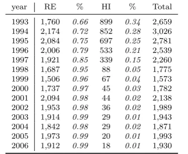
The DHS is an unbalanced panel. As reported in Table 1, when the survey started, it

consisted of two panels, one representative of the Dutch population (RE), covering 1,760 households, and the other representative of the top 10 percent of the income distribution

(HI), encompassing approximately 900 families, with a share of 66% and 34%, respectively. The last wave of the panel consists of 1,800 households in the RE panel and only 29 in

the HI panel. The severe reduction in the HI panel is due to the fact that since 1997 new families have not been recruited for the HI panel, so it quickly shrank as the higher income families exited the panel.

Table 1: Number of households by panel type and year

year RE % HI % Total 1993 1,760 0.66 899 0.34 2,659 1994 2,174 0.72 852 0.28 3,026 1995 2,084 0.75 697 0.25 2,781 1996 2,006 0.79 533 0.21 2,539 1997 1,921 0.85 339 0.15 2,260 1998 1,687 0.95 88 0.05 1,775 1999 1,506 0.96 67 0.04 1,573 2000 1,737 0.97 45 0.03 1,782 2001 2,094 0.98 44 0.02 2,138 2002 1,953 0.98 36 0.02 1,989 2003 1,914 0.99 29 0.01 1,943 2004 1,842 0.98 29 0.02 1,871 2005 1,973 0.99 20 0.01 1,993 2006 1,912 0.99 18 0.01 1,930

Notes: Column RE reports summary statistics for the panel representative of the Dutch population. Column HI reports summary statistics for the panel representative of the top 10 percent of the income distribution of the

Dutch population.

The DHS consists of six questionnaires, presented to all the people aged 16 or over

within the family, that collect detailed information on demographics, work, health status,

family composition, individual and family incomes and wealth.3 Moreover, the DHS is one of the few surveys that collects different kinds of subjective expectations on the future

family income, inflation and information on agents’ attitudes toward risk and their time preferences. Being a saving survey, the DHS panel doesn’t collect data on consumption

directly, but the wide variety of data on saving and income makes us possible to construct alternative estimates of consumption.

The panel runs from 1993 to 2006.4 _{Each wave contains flow and stock information for}

the previous year. The period we consider in our analysis runs from 1995 to 2002, as some variables of interest have been collected only in these years. In the next section, we focus on

some variables derived from the subjective information in the questionnaire. These variables are the household’s expected income, realized income and savings. Expectations concerning the next year’s income level were obtained by reports of the subjective probabilities that it

will fall in intervals. Using two different parametric assumption, we estimate the subjective probability distribution over next year’s income. Measures of realized income are obtained

either from reports of income categories or by applying self reported income growth rates to earlier income measurements. Savings are reported by category.

3.1 The probability distribution of next years family income

The data on expected next year income are collected by a module that is similar to the one

adopted in the Survey of Economic Expectations (SEE), and discussed in Dominitz and Manski (1997).

In the DHS, the respondents are first asked to answer two questions about the range in which their family income is expected to fall in the next twelve months; the precise wording, translated into English by CentER, is the following: What do you expect to be

the lowest (highest) total net income your household may realize in the next 12 months?.

After answering these questions the interview software determines four income thresholds

by means of the following algorithm: thresholdκ = Ymin+ 0.2κ(Ymax −Ymin) and κ = 1, ...4. Then, the respondents are asked to report the percent chance that their net family income will be betweenYmin and each threshold. The precise wording of the question is as follows:What do you think is the probability that the total net income of your household will

3_{The survey method is completely computerized. Each household is provided with a personal computer,}

receives the questionnaires by modem, answers the questionnaires on its home computer and returns the answers to the CentER by modem again. This means that the questionnaires are self-administered and the respondents can answer the questionnaires at a time that is convenient for them.

Table 2: Number of respondents at the questions on lowest and highest possible income and cumulative subjective probability distribution and response rates

Year 1995 1996 1997 1998 1999 2000 2001 2002 Pooled household 4854 4250 3447 2392 2250 1055 2075 2139 22462

Ymax, Ymin 2335 2035 2847 1966 1863 1037 2043 2095 16221

% 0.48 0.48 0.83 0.82 0.83 0.98 0.98 0.98 0.72

Ymax−Y_min<5 323 293 339 239 245 135 338 365 2277

% 0.07 0.07 0.10 0.10 0.11 0.13 0.16 0.17 0.10

Probab. 2010 1741 2195 1483 1372 899 1709 1732 13141

% 0.41 0.41 0.64 0.62 0.61 0.85 0.82 0.81 0.59

No monoton. 307 295 311 212 202 184 352 388 2251

% 0.06 0.07 0.09 0.09 0.09 0.17 0.17 0.18 0.10

Final 1703 1446 1884 1271 1170 715 1357 1344 10890 % 0.35 0.34 0.55 0.53 0.52 0.68 0.65 0.63 0.48

be less than threshold k in the next 12 months? Please fill in a number between 0 to 100.5

After division by 100, we obtain 4 point values, corresponding to the thresholds, for the

subjective cumulative distribution function of next year’s net family income. We will make two different assumptions on the subjective distribution of the respondents. Because of the

structure of the questionnaire, we decided to use distributions with bounded support: the beta and the piecewise linear. The beta is estimated by non-linear least squares.

The questionnaire on health and income, containing the module described above, was presented to a decreasing number of respondents during the period that goes from 1995 to 2000 and to around 2,000 individuals in the subsequent years. As shown in Table 2, 72%

of the respondents stated at least Ymin and Ymax. It should be underlined that they were not asked the subsequent questions if the difference between Ymax and Ymin was smaller than a fixed amount which corresponds to 5 Dutch florins (dlf.) until 2002 and 5 euros for the following years. This is the case for 2277 observations (10%).

The DHS suffers a problem of non monotonicity in the stated subjective cumulative

distribution function. The cases which present this problem are 2251 (10%). A brief analysis of the answers reveals that some people are not able to articulate their expectations using

the theory of probability and/or commit typing and recording errors. The final response rate is around half (48%) of respondents. It is small for the first two years (35%), but

increases over time to 63%.

The analysis of the lowest and highest possible incomes reveals that 64 respondents have declared a highest possible income inferior to 100 euros and 14 far superior to 500,000 euros.

These values seem implausible to us and we decide to drop the corresponding observations.

5_{The percent chance of}

The mean value of the lowest possible income is e_{18,587 with stated values that vary from}

0 to 385,900, while the mean value of the highest possible income is e_{23,176 in a range}

that goes from 100 to 500,000.

3.2 Measuring consumption

An important feature of the data concerns the way consumption is estimated since it is not directly observed. Consumption can be defined as the difference between income and

savings.

In our empirical analysis, we use respondent’s answers on self reported family savings. In particular, we refer to a pair of questions that are part of the section on psychological

concepts which we report below:

Did you put any money aside in the past 12 months?

If the answer is yes, the respondent is also asked the following question about the amount:

About how much money has your household put aside in the past 12 months? 0 don’t know

1 less than Dfl. 3,000 (e_1361,34)

2 3,000 - 10,000(e_{1361,34 and} e_4537,80)

3 10,000 - 25,000 (e_{4537,80 and} e_11344,51)

4 25,000 - 40,000 (e_{11344,51 and} e_18151,21)

5 40,000 - 75,000 (e_{18151,21 and} e_34033,52)

6 75,000 - 150,000 (e_{34033,52 and} e_68067,03)

7 150,000 or more (e_68067,03)

Because of the difficulty in providing accurate responses to questions about either

earn-ings, income, savings and wealth, and in order to reduce the rate of item non-response, surveys have increasingly used classes as possible answers. Here, respondents are expected to report the amount of money put aside by choosing one of the seven predetermined classes

or the non-informative ”don’t know”. Out of this information we have constructed a vari-able by taking the midpoints of each class. Since the last interval is right censored, no

A possible source of data on income comes from CentER which aggregates self reported financial information in order to calculate a comprehensive personal income measure.

How-ever, they correctly sum up all the different types of income, while respondents, making predictions, may refer only to the more important family income components such as

wages.6 This could cause a systematic bias in the forecast error. Indeed, forecast income is on average significantly lower than income as measured by CentER. Moreover, differences across households in the set of income components considered when forecasting income

would, in effect, add noise or measurement error to the forecasts. For these reasons we choose to deal with the available self reported information on household net income. This

should help to avoid spurious evidence against the null hypotheses of rational expectations formation.

Here, an estimate of income is obtained by the transformation of the self reported

realized income growth. The respondents are asked to answer a first preliminary question on their income growth, that is the following:

Compared to about one year ago, did the total net income of your household increase, remain about the same, or decrease?

The possible answers to such a question are: increase, remain the same, decrease. If the

re-spondents indicates either an increase or a decrease, he is asked the following supplementary question:

By what percentage (approximately) has the total net income of your household

increased(decreased)?

Thus, it is possible to construct a variable representing the growth rate of total household

net income, that takes values equal to the declared percentages if the respondent indicates an increase or a decrease, or that takes value 0 if he reports total net family income to

remain the same.

Hence, we apply the following simple formula for the first wave where answers are

provided

yt=zt−1∗(1 +

gt

100) (19)

6_{CentER also allows for processes of grossing-up when only net income components are available.}

wherey represents the subjective realized income;z1995 is the initial value of the family

income, as aggregated by CentER summing the incomes of all the family’s members; g is the self reported income growth rate. For the subsequent waves,zis equal to the previously obtained estimate of income, that iszt−1 =yt−1. For new entrants and re-entrants in wave

t−1,yt−1 is family income as aggregated by CentER andyt is constructed using Eq. (19) where we set zt−1 =yt−1.

Finally, we also construct an alternative estimate of family income which is derived

from a question where respondents are asked to indicate the interval which corresponds to the income realized over the last year 12 months. The precise wording of the question is

reported below:

Into which of the categories mentioned below did the total net income of your household go in the past 12 months? If you really don’t know, use ”don’t know”.

0 don’t know

1 less than Dfl. 20,000 (e_9075,60)

2 20,000 - 28,000 (e_{9075,60 and} e_12705,85)

3 28,000 - 43,000 (e_{12705,85 and} e_19512,55)

4 43,000 - 80,000 (e_{19512,55 and} e_36302,42)

5 80,000 - 150,000 (e_{36302,42 and} e_68067,03)

6 150,000 or more (e_68067,03)

The estimate of income is constructed similarly to estimated savings assigning the midpoints of the intervals indicated by the respondent. For the respondents that indicate

the sixth interval, as above we assign the value of e_{100,000 as the highest bound. We}

subtract subjective expected next year’s income from this income estimate to calculate the

error in predicting future income.

As shown in Table 3, on average 87% of all respondents answered to the questions on the family income growth and level. Response rates are smaller for the modules on savings

(63%). We dropped a few observations characterized by implausible values of the declared income growth rate.7 _{After these deletions, the mean value of the self reported income}

growth rate is positive and amounts to 1.2% with stated percentages that vary from -100 to 200.

Our analysis is based on data from most of the questionnaires of the DHS panel. In

7_{9 respondents declared a growth rate greater than 200% and 4 declared a reduction greater than 100%,}

Table 3: Number of respondents at the questions on realized family income growth, income level and savings, and response rates

Year Household Income % Income % Savings %

growth

1995 4055 3675 0.91 3675 0.91 2672 0.66

1996 3384 3091 0.91 3091 0.91 2215 0.65

1997 2660 2417 0.91 2417 0.91 1661 0.62

1998 1365 1264 0.93 1264 0.93 867 0.64

1999 1368 1300 0.95 1300 0.95 937 0.68

2000 1934 1349 0.70 1349 0.70 1002 0.52

2001 2663 2097 0.79 2097 0.79 1624 0.61

2002 2358 1994 0.85 1993 0.85 1560 0.66

Total 19787 17187 0.87 17186 0.87 12538 0.63

particular, it draws heavily upon the part on health and income, where subjective expec-tations on next year’s income were collected, and upon the part on psychological concepts

where subjective inflation forecasts and self reported previous years realized income, real-ized income growth, and savings were collected.

The sample used in the empirical analysis below includes only heads of households, who

are less than 100 years of age. To estimate the model, we need at least three consecutive waves of data. Since some questions of interest on subjective income were collected only

from 1995 to 2002, we only consider eight waves. We do not make use of imputation in the cases of item non response. Instead we drop the families for which variables on expected

and realized income are not available. Other observations are not considered due to lack of data on relevant variables such as sex, age, education, etc., but they are very few and substantially negligible.

Merging the data from all the questionnaires produces a pooled data set for all waves which contains 7383 individuals. However, since we use only observations that remain

in the panel for at least three consecutive years, the number of available respondents is reduced to 3062. 1120 of them remain in the panel for only three waves while 75 stay for

the entire duration of the panel. The mean duration is 2.7 with the first and third quartiles of the distribution equal to 1 and 4.

To deal with the fact that subjective expectations are characterized by the presence of

4

Empirical implementation of the model and testing

pro-cedure

We estimate the model presented in section 2 using instrumental variables in order to test

the null of rational expectations and isoelastic seperable utility. The idea is that non ratio-nal pessimistic/optimistic agents commits systematic errors in forecasting income, which

can be predicted by the econometrician. Agents that have been irrationally pessimistic ex-perience a positive surprise when income is realized and revise their consumption decisions

up. Conversely, irrationally optimistic agents experience a bitter surprise and downward revise their consumption decisions down.

To implement the theoretical statement we use a two step procedure. In the first stage,

we instrument forecast errors. That is, we run an orthogonality test regressing forecast errors on data that were in the agents’ information set at the time the expectations were

stated. All it is required for a variable to be a good instrument is that it is exogenous with respect to the dependent variable. This requirement is automatically met under the null for all the data that were part of the information set of the agent when he stated

his expectations. If the null of rational expectations is rejected, we are able to predict agents’forecast errors, that is, the systematic surprises that they experience as income

realizes. Thus we test our behavioral model of consumption, estimating the modified Euler equation presented in the Eqs. 15 and 18, as the second step of the procedure.

4.1 The first stage

Considering expectations on the growth rate of income, a general first stage orthogonality

test have the following form:

yt+1−Etsu(yt+1) =Xtβˆ+Ztˆγ+ǫt+ 1 (20)

whereXtis a matrix of data contained in the agents’ information set andZtis a matrix of controls. Under the null of rational expectations β = 0 and γ = 0. We refer to the left hand side of Eq. 20, yt+1−Etsu(yt+1), as the forecast error.

No model that explains the alternative to the null hypotheses is specified8.

For our purposes the main limitation of our panel remains its short time dimension, that

8_{Our theoretical model, and the empirical evidence that will be furnished in the next sections are perfectly}

is 8 years. The conditional expectation of the disturbance terms E(ǫt+1), according with

permanent income hypothesis with rational expectations, must be zero. The empirical

analog of E(ǫt+1) is an average calculated on a long time span, in fact, as pointed out

by Chamberlain (1984), the increase of the cross section dimension do not guarantee its

convergence to zero. Even though the forecast error should be zero on average if calculated on a long time period, this may not be the case in short panels. Otherwise stated, when performed with short panels, the orthogonality test, is a joint test of the orthogonality

condition and of the maintained assumption that forecast errors are not correlated across households. Rejection of the null in favor of our behavioral model, may be attributed to

the inconsistency of the estimator. To control for macroeconomic shocks we have included controls in both steps of the estimation procedure. In particular we allow for the presence of time and geographical dummies.

The choice between regressors and controls is someway arbitrary and controls cannot be used to test the null. Hence, we allow for different specifications.

As underlined above, we have information on the subjective maximum and minimum expected income and on the subjective cumulative distribution function of next year’s net

family income, calculated at the thresholds. That makes as possible to estimate the entire distribution of income expectations without making assumptions on the shape of the loss function. Hence, the rejection of the null in our orthogonality test is never imputable to false

assumptions on the loss function. The only assumption that our analysis requires is on the distribution function whose parameters have to be estimated. To understand whether this

choice have an effect on our estimates, we allow for two alternative distribution functions: the beta and the piecewise uniform.

4.2 Second stage: the Euler equation

If the hypothesis of rational expectations is rejected, we test our behavioral model of

consumption estimating the following Euler equation:

log(ct+1

ct

) =α1Xˆtβ+α2V arsut (yt+1) +α3Etsuπt+1+γ(controls) +ηt+1 (21)

whereXtβ is the predicted forecast error, V arsut (yt+1) is the variance of the subjective

distribution of next year family income andE_tsuπt+1is the subjective inflation expectation.

The conditional variance term is included in the regression to allow for the fact that

depends on prudence, reduce consumption now with respect to future as reaction to an increase in consumption risk. Ludvingson and Paxson (1997) and Jappelli and Pistaferri

(2000) have pointed out that the failure to properly taking into account consumption risk will bias the coefficient of the inter-temporal elasticity of substitution, and, furthermore

it will generate spurious evidence of excess sensitivity. The same reasoning applies to our behavioral model.

We have also included the expected inflation, Esu

t πt+1. Theoretically, the expected

values of the real interest rate should enter the Euler equation, as a relevant variable in saving decision. Our data set do not collect subjective expectations about next year real

interest rate, but it is possible to proxy it by using expected inflation. This approximation is exact if financial market is perfect. In this case there is only one interest rate and subjective expected real interest rates differ only because of inflation expectations.

The main limitation of our panel continues to be its short time dimension that makes it susceptible of the Chamberlain(1984)’s critique. As summarized by Jappelli and Pistaferri

(2000), the excess sensitivity test, when performed on a short panel is a joint test of the null and of an assumed structure of the disturbance term,ηt+1. Apparent excess sensitivity may

arise as the result of not properly taking into account the cross correlation of disturbances. To control for evenly and unevenly distributed macroeconomic shocks we have included controls in both steps of the estimation procedure. In particular, we allow for the presence

of time dummies and geographical dummies .

Another problem may arise because of the failure of the separability assumption. If

consumption and leisure are not separable, today’s decision will be affected by predictable changes in households’ labor supply. This implies that consumption is correlated with

hours of work, which are in turn correlated with income growth. Failure to consider for non separability may bring us to spurious evidence of excess sensitivity. Therefore, among the controls at the second step we have explicitly included variables describing variations

in the number of family components, components that are looking for a job and income recipients.

5

Results

In this section we present the empirical evidence concerning the model presented in section

To deal with the noise contained in the measured income and savings, and hence in measured consumption, and with the extreme values contained in the subjective

expec-tations we have run a robust estimator. The estimator is robust with respect to outliers either in the space of the regressors and in the space of residuals.9

The null is rejected with both OLS and the robust estimator. We use the robust estimates as our linear prediction of the systematic error component to use in the second step.

The assumption of rational expectations implies that our instruments are weakly ex-ogenous, so long as we use instruments that were in the agents’ information sets. In order

to show that our results are not due to a particular set of instruments we use alternative sets.

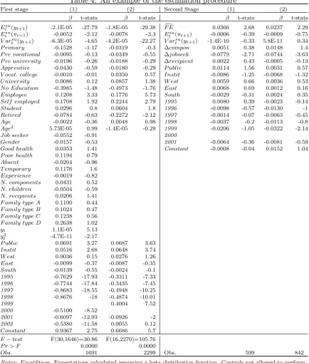
Table 4 shows an example of our regressions. Forecast errors are defined as the difference

between the self reported income realizations, calculated as the midpoints of the reported intervals, at time t+ 1 and the subjective mean of next year’s family income level at time

t calculated assuming a beta distribution function.

The first two columns report results for two alternative specifications of the first stage.

The reported P-value for both the regressions reject the hypothesis of rational expectations at any conventional significance level. The last columns report results for the estimation of the corresponding second stage Euler equations. Both shows that predictable forecast

errors help explain consumption variations which is evidence in favor of our behavioral model.

Let’s look at the reported first stages. We start, in the first column, regressing the forecast error on a huge amount of regressors and on a set of controls. This set of controls

is the same we allow at the second stage and that is reported in the last two columns. Regressors include variables on household’s structure, income, and variables describing the head of the household. The reported F-test is based on the set of regressors but not on the

controls.

There is a significant negative coefficient on expected income, which may reflect the

fact that people that have been too optimistic are going to experience a bitter surprise in the realization and the converse if they have been too pessimistic.

The choice between regressors and controls is someway arbitrary, so we have calculated

the F test on different sub-samples of the regressors. For example, considering as controls

9_{The results that will be presented in following tables have been obtained by using the}

Table 4: An example of the estimation procedure

First stage (1) (2) Second Stage (1) (2)

β t-stats β t-stats β t-stats β t-stats

Esu

t (yt+1) -2.1E-05 -27.79 -1.8E-05 -29.38 F Ed 0.0366 2.68 0.0237 2.29

Esu

t (πt+1) -0.0052 -2.12 -0.0078 -3.3 Etsu(πt+1) -0.0006 -0.39 -0.0009 -0.75

V arsu

t (yt+1) -6.3E-05 -4.65 -4.2E-05 -22.27 V arsut (yt+1) -1.4E-10 -0.33 5.8E-11 0.34

P rimary -0.1528 -1.17 -0.0319 -0.3 ∆compon 0.0051 0.38 0.0148 1.4

P re vocational -0.0095 -0.13 -0.0349 -0.55 ∆jobseek -0.0779 -2.71 -0.0744 -3.63

P re university -0.0196 -0.26 -0.0188 -0.29 ∆recipient 0.0022 0.43 -0.0005 -0.13

Apprentice -0.0430 -0.59 -0.0180 -0.29 P ublic 0.0114 1.56 0.0031 0.57

V ocat. college -0.0010 -0.01 0.0350 0.57 Instit -0.0086 -1.25 -0.0068 -1.32

U niversity 0.0086 0.12 0.0857 1.38 W est 0.0059 0.66 0.0036 0.53

N o Education -0.3985 -1.48 -0.4973 -1.76 East 0.0068 0.69 0.0012 0.16

Employee 0.1208 3.33 0.1776 5.73 South -0.0029 -0.31 0.0024 0.35

Self employed 0.1708 1.92 0.2244 2.79 1995 0.0080 0.39 -0.0023 -0.14

Student 0.0296 0.8 0.0604 1.8 1996 -0.0098 -0.57 -0.0130 -1

Retired -0.0784 -0.63 -0.2272 -2.12 1997 -0.0014 -0.07 -0.0063 -0.45

Age -0.0022 -0.36 0.0048 0.98 1998 -0.0037 -0.2 -0.0113 -0.8

Age2 _{5.73E-05 0.99 -1.4E-05 -0.29 1999 -0.0206 -1.05 -0.0322 -2.14}

Job seeker -0.0552 -0.91 2000

Gender -0.0157 -0.53 2001 -0.0064 -0.36 -0.0081 -0.59

Good health 0.0353 1.41 Constant -0.0008 -0.04 0.0152 1.04

P oor health 0.1194 0.79

Absent -0.0204 -0.96

T emporary 0.1176 1.6

Experience -0.0019 -0.82

N. components 0.0431 0.52

N. children -0.0504 -0.59

N. recipients 0.0206 1.41

F amily type A 0.1100 0.44

F amily type B 0.1024 0.47

F amily type C 0.1238 0.56

F amily type D 0.2638 1.02

yt 1.1E-05 5.13 y2

t -4.7E-11 -2.17

P ublic 0.0691 3.27 0.0687 3.63

Instit 0.0516 2.68 0.0648 3.74

W est 0.0036 0.15 0.0276 1.26

East -0.0099 -0.37 -0.0087 -0.35

South -0.0139 -0.55 -0.0024 -0.1

1995 -0.7629 -17.93 -0.3311 -7.33

1996 -0.7744 -17.84 -0.3435 -7.45

1997 -0.8683 -18.55 -0.4948 -10.25

1998 -0.8676 -18 -0.4874 -10.01

1999 0.4004 7.52

2000 -0.5100 -8.52

2001 -0.6097 -12.93 -0.0926 -2

2002 -0.5380 -11.58 0.0055 0.12

Constant 0.9367 2.75 0.6686 5.7

F−test F(30,1646)=30.86 F(16,2270)=105.76

P r > F 0.0000 0.0000

Obs. 1691 2299 Obs. 599 842

Notes: F irstStage. Expectations calculated assuming a beta distribution function. Controls not allowed to perform prediction and the F-test. Esu

t (πt+1) inflation expectation (point expectation). Job seekeris an indicator variable

for looking for a job.Genderis an indicator variable that takes value 1 if respondent is male. Absentis an indicator variable for being absent from work because of illness last year. T emporary is an indicator that takes value 1 if employed on a temporary basis. Experienceis years of work since the first occupation. N. components,N. children

and N. recipients are variables on number of family components, children and income recipients in the family. VariablesF amily type A−D are indicators for: single, with partner and without children, with partner and with

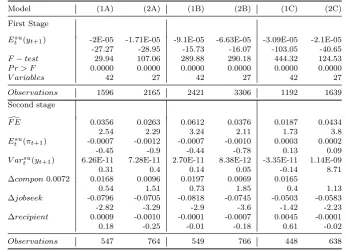
Table 5: Estimation results assuming a beta distribution

Model (1A) (2A) (1B) (2B) (1C) (2C) First Stage

Esu

t (yt+1) -2.1E-05 -1.8E-05 -8.6E-05 -6.3E-05 -3.1E-05 -2.1E-05

-27.79 -29.38 -16.26 -16.47 -105.45 -41.38

F−test 30.86 105.76 309.11 307.95 464.57 127.13 P r > F 0.0000 0.0000 0.0000 0.0000 0.0000 0.0000

V ariables 43 28 43 28 43 28

Observations 1691 2299 2656 3641 1301 1792

Second stage d

F E 0.0366 0.0237 0.0585 0.0323 0.0130 0.0402 2.68 2.29 3.02 1.92 1.24 3.78

Esu

t (πt+1) -0.0006 -0.0009 -0.0005 -0.0008 0.0006 0.0004

-0.39 -0.75 -0.33 -0.63 0.27 0.22

V arsu

t (yt+1) -1.38E-10 5.82E-11 -8.00E-11 -4.02E-12 -5.07E-10 1.11E-09

-0.33 0.34 -0.2 -0.02 -0.87 8.89 ∆compon 0.0052 0.0148 0.0075 0.0177 0.0056 0.0142 0.38 1.4 0.58 1.74 0.32 1.01 ∆jobseek -0.0779 -0.0744 -0.0824 -0.0780 -0.0502 -0.0615 -2.71 -3.63 -2.90 -3.92 -1.38 -2.41 ∆recipient 0.0022 -0.0005 0.0019 -0.0002 0.0082 0.0015 0.43 -0.13 0.38 -0.05 1.12 0.28

Observations 599 842 602 845 497 708

Notes: Models labelled with (1) allow for the large set of instruments at the first stage. Models labelled with (2) allow for the smaller set of instruments. In Model A, forecast errors are defined as the difference between the self reported income realizations, calculated as the midpoints of the reported intervals, at timet+ 1 and the subjective mean of next year’s family income level at timetcalculated assuming a beta distribution function. In model B, forecast errors are defined as a binary variable that takes the unit value if the minimum declared realized income is higher than the expected income level. In Model C, forecast errors are computed as the difference between family income realizations from self reported income growth rates and subjective family income expectations. Control variables are not used to perform the F-test. dF Eis predicted forecast error. Esu

t (πt+1) inflation expectation (point expectation). ∆compon

controls for the variation in family composition. ∆jobseekcontrols for the variation in the number of family members who declare to be looking for a job. ∆recipientcontrols for the variation in the number of income recipients in the family.

all the variable with the exception of those that we also use in the second column gives a

F(26,1890) = 59.76 which rejects the null at any conventional level. The extreme possi-bility is to consider the stated expectation as the only regressor completely immune to the

influence of macroeconomic shocks and all the other variables as controls. In this case the orthogonality test reduces to a t-test. Reported results continue to support the rejection of the null even in this last case.

The second column report results for an alternative specification of the information set. Here we consider a smaller subset of regressors but taking use of the same set of controls.

The reason for doing so is to avoid over-prediction in the IV estimator. If that were the case, our predicted forecast error may capture events that were genuinely unpredictable,

resulting in spurious evidence in favor of our behavioral model.

forecast-Table 6: Estimation results assuming a piecewise linear distribution

Model (1A) (2A) (1B) (2B) (1C) (2C) First Stage

Esu

t (yt+1) -2.1E-05 -1.8E-05 -8.8E-05 -6.5E-05 -3.1E-05 -2.2E-05

-33.91 -35.22 -17.03 -17.25 -103.44 -48.71

F−test 51.97 388.36 330.12 336.16 450.35 200.57 P r > F 0.0000 0.0000 0.0000 0.0000 0.0000 0.0000

V ariables 43 28 43 28 43 28

Observations 1791 2434 2795 3830 1387 1905 Second stage

d

F E 0.0383 0.0265 0.0630 0.0343 0.0159 0.0390 2.95 2.6 3.52 2.12 1.62 3.88

Esu

t (πt+1) -0.0007 -0.0010 -0.0006 -0.0009 0.0002 -0.0003

-0.43 -0.83 -0.42 -0.72 0.1 -0.16

V arsu

t (yt+1) 1.4E-10 9.1E-11 4.1E-11 3.4E-12 -1.9E-10 1.1E-09

0.33 0.53 0.1 0.02 -0.35 9.14 ∆compon 0.0083 0.0167 0.0115 0.0196 0.0071 0.0159 0.65 1.59 0.92 1.95 0.43 1.18 ∆jobseek -0.0459 -0.0565 -0.0497 -0.0603 -0.0518 -0.0602 -1.73 -2.82 -1.88 -3.12 -1.48 -2.39 ∆recipient 0.0005 -0.0005 0.0003 -0.0001 0.0061 0.0019 0.1 -0.13 0.07 -0.03 0.89 0.34

Observations 625 877 628 880 520 739

Notes: Models labelled with (1) allow for the large set of instruments at the first stage. Models labelled with (2) allow for the smaller set of instruments. In Model A, forecast errors are defined as the difference between the self reported income realizations, calculated as the midpoints of the reported intervals, at timet+ 1 and the subjective mean of next year’s family income level at time tcalculated assuming a piecewise linear distribution function. In model B, forecast errors are defined as a binary variable that takes the unit value if the minimum declared realized income is higher than the expected income level. In Model C, forecast errors are computed as the difference between family income realizations from self reported income growth rates and subjective family income expectations. Control variables are not used to perform the F-test. F Ed is predicted forecast error. Esu

t (πt+1) inflation expectation (point

expectation). ∆componcontrols for the variation in family composition. ∆jobseekcontrols for the variation in the number of family members who declare to be looking for a job. ∆recipientcontrols for the variation in the number of income recipients in the family.

ing income, F Ed, explain consumption variation, confirming that irrational pessimistic/ optimistic consumers upward/downward revise their consumption decision as income real-izes. The omission of some instruments in the first step gives smaller estimated coefficients

on predictable forecast errors but they are still significant at the 5% level. The coefficient on expected inflation is not statistically significant, while the change in the number of

household’s components who seek a job has a negative and significant coefficient. Controls are not statistically significant, except for the dummy of year 1999 in the case with fewer

regressors.

When we omit indicators of educational qualifications from the model with a smaller set of regressors, we obtain similar coefficients with smaller t-statistics. This evidence is

consistent for alternative specifications.

follow the convention of labelling (1) the results obtained allowing for the large set of in-struments at the first stage, and (2) those obtained with the smaller set of inin-struments. For

every orthogonality test, we have reported the estimated coefficients of expected income, the number of observations, the number of variables and the F-test results. Second stage

results constitute of the estimated coefficients of predictable forecast errors, expected in-flation, subjective income variance,V ar_tsu(yt+1), and controls for non separability between

consumption and leisure. Model A refers to the estimates that we have already presented

in Table 4. In models B and C we produce alternative estimates of forecast error. In model B, forecast errors are defined as a binary variable that takes the unit value if the minimum

declared realized income is higher than the expected income level. In Model C, forecast errors are computed as the difference between family income realizations from self reported income growth rates, as calculated in Eq. 19, and subjective family income expectations.

To show that our results are not driven by the choice of the subjective expectations dis-tribution function we reported, in Table 6, results referring to the same models described

above for the case of a piecewise linear distribution function.

The estimated coefficient of predictable forecast error is always positive and

statisti-cally significant at the 5 percent level, with values from 0.024 to 0.063. It is smaller when we consider the specification with a smaller set of instruments. Model C exhibits slightly different results, as the forecast error coefficient is still positive but smaller and not

sig-nificant at 5% in case (1). Although we are not able to give a structural interpretation of the parameters, our estimates show that non separability of consumption and leisure

may be important in consumption decision, particularly as variations in the number of job seekers, ∆jobseek, and components, ∆compon, in a household may have an impact. On the contrary, precautionary savings and interest rates appear to be less important.

As shown in Figure 1, we observe significant shifts to upper classes in the reported income categories between 1999 and 2000, while, the distribution of answers is stable along

the other years. The magnitude of this change is huge, as the mean of household’s income level jumps from e_{25,310 in 1999 to} e_{42,193 in 2000 (Figure 2). In order to understand}

whether and how this unexpected and anomalous shock influences our findings, we drop all observations of year 1999, with which the change from 1999 to 2000 is associated, and replicate all regressions. We perform this for both the regressors’ specifications. Results,

reported in Tables 7 and 8, confirm our previous findings, showing again an estimated coefficient of predictable forecast error positive and significant, and with value between

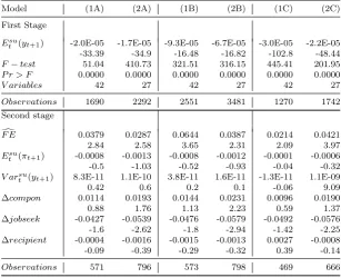
Table 7: Estimation results assuming a beta distribution. Year 1999 dropped

Model (1A) (2A) (1B) (2B) (1C) (2C) First Stage

Esu

t (yt+1) -2E-05 -1.71E-05 -9.1E-05 -6.63E-05 -3.09E-05 -2.1E-05

-27.27 -28.95 -15.73 -16.07 -103.05 -40.65

F−test 29.94 107.06 289.88 290.18 444.32 124.53 P r > F 0.0000 0.0000 0.0000 0.0000 0.0000 0.0000

V ariables 42 27 42 27 42 27

Observations 1596 2165 2421 3306 1192 1639

Second stage d

F E 0.0356 0.0263 0.0612 0.0376 0.0187 0.0434 2.54 2.29 3.24 2.11 1.73 3.8

Esu

t (πt+1) -0.0007 -0.0012 -0.0007 -0.0010 0.0003 0.0002

-0.45 -0.9 -0.44 -0.78 0.13 0.09

V arsu

t (yt+1) 6.26E-11 7.28E-11 2.70E-11 8.38E-12 -3.35E-11 1.14E-09

0.31 0.4 0.14 0.05 -0.14 8.71 ∆compon0.0072 0.0168 0.0096 0.0197 0.0069 0.0165

0.54 1.51 0.73 1.85 0.4 1.13 ∆jobseek -0.0796 -0.0705 -0.0818 -0.0745 -0.0503 -0.0583 -2.82 -3.29 -2.9 -3.6 -1.42 -2.23 ∆recipient 0.0009 -0.0010 -0.0001 -0.0007 0.0045 -0.0001 0.18 -0.25 -0.01 -0.18 0.61 -0.02

Observations 547 764 549 766 448 638

Notes: Observations for the year 1999 dropped. Models labelled with (1) allow for the large set of instruments at the first stage. Models labelled with (2) allow for the smaller set of instruments. In Model A, forecast errors are defined as the difference between the self reported income realizations, calculated as the midpoints of the reported intervals, at timet+ 1 and the subjective mean of next year’s family income level at timetcalculated assuming a beta distribution function. In model B, forecast errors are defined as a binary variable that takes the unit value if the minimum declared realized income is higher than the expected income level. In Model C, forecast errors are computed as the difference between family income realizations from self reported income growth rates and subjective family income expectations. Control variables are not used to perform the F-test. dF Eis predicted forecast error.

Esu

t (πt+1) inflation expectation (point expectation). ∆compon controls for the variation in family composition.

∆jobseekcontrols for the variation in the number of family members who declare to be looking for a job. ∆recipient

controls for the variation in the number of income recipients in the family.

Results are still in line with our hypothesis when we eliminate the subjective income

variance from all sets of regressors of first steps and second steps, whether or not we include data from 1999, as is shown in Tables 10 and 11. Indeed, the significative parameters

associated to the predicted income error take values between 0.021 and 0.064, similarly to the cases examined above. The same results have been obtained assuming a piecewise linear distribution function and, for the ease of exposition, have not been reported.10

6

Irrationality and excess sensitivity

In this section we investigate the relative importance of irrationality, liquidity constraints, and precautionary saving in explaining excess sensitivity.

Table 8: Estimation results assuming a piecewise linear distribution. Year 1999 dropped

Model (1A) (2A) (1B) (2B) (1C) (2C) First Stage

Esu

t (yt+1) -2.0E-05 -1.7E-05 -9.3E-05 -6.7E-05 -3.0E-05 -2.2E-05

-33.39 -34.9 -16.48 -16.82 -102.8 -48.44

F−test 51.04 410.73 321.51 316.15 445.41 201.95 P r > F 0.0000 0.0000 0.0000 0.0000 0.0000 0.0000

V ariables 42 27 42 27 42 27

Observations 1690 2292 2551 3481 1270 1742 Second stage

d

F E 0.0379 0.0287 0.0644 0.0387 0.0214 0.0421 2.84 2.58 3.65 2.31 2.09 3.97

Esu

t (πt+1) -0.0008 -0.0013 -0.0008 -0.0012 -0.0001 -0.0006

-0.5 -1.03 -0.52 -0.93 -0.04 -0.32

V arsu

t (yt+1) 8.3E-11 1.1E-10 3.8E-11 1.6E-11 -1.3E-11 1.1E-09

0.42 0.6 0.2 0.1 -0.06 9.09 ∆compon 0.0114 0.0193 0.0144 0.0231 0.0096 0.0190 0.88 1.76 1.13 2.23 0.59 1.37 ∆jobseek -0.0427 -0.0539 -0.0476 -0.0579 -0.0492 -0.0576 -1.6 -2.62 -1.8 -2.94 -1.42 -2.25 ∆recipient -0.0004 -0.0016 -0.0015 -0.0013 0.0027 -0.0008 -0.09 -0.39 -0.29 -0.32 0.39 -0.14

Observations 571 796 573 798 469 666

Notes: Observations for the year 1999 dropped. Models labelled with (1) allow for the large set of instruments at the first stage. Models labelled with (2) allow for the smaller set of instruments. In Model A, forecast errors are defined as the difference between the self reported income realizations, calculated as the midpoints of the reported intervals, at timet+ 1 and the subjective mean of next year’s family income level at timetcalculated assuming a piecewise linear distribution function. In model B, forecast errors are defined as a binary variable that takes the unit value if the minimum declared realized income is higher than the expected income level. In Model C, forecast errors are computed as the difference between family income realizations from self reported income growth rates and subjective family income expectations. Control variables are not used to perform the F-test. F Ed is predicted forecast error. Esu

t (πt+1) inflation expectation (point expectation). ∆componcontrols for the variation in family

composition. ∆jobseekcontrols for the variation in the number of family members who declare to be looking for a job. ∆recipientcontrols for the variation in the number of income recipients in the family.

Theoretically, the rejection of the hypothesis that consumption is a random walk can be

attributed to the presence of liquidity constraints, precautionary savings and irrationality or myopia. Oddly, in the extensive literature on testing the permanent income

hypothe-sis, the possibility that rejection is due to predictable forecast errors is rarely mentioned, let alone explored. From Hall’s article (Hall, 1978) on, all the effort in testing the Euler equation and excess sensitivity of consumption to predictable income changes have

con-centrated on liquidity constraints and precautionary saving, although, as pointed out by Carroll (1992), it is very hard to distinguish empirically between precautionary saving and

liquidity constraints as households may increase saving today if they expect to be liquidity constrained in the future.

sources of excess sensitivity.

We estimate the following Euler equation, modified to allow for irrationality.

∆lnCt+1=α∆Dt+1+ρ

−1

(E(rt+1|Ωt)−δ)+

ρ

2vart(∆lnCt+1−ρ −1

(rt+1))+

βE∆ln(yt+1|Ωt) +γE[yt+1−Etsu(yt|Ωt)] +εt+1, (22)

whereiis an household index,Ci,t+1 is our estimate of consumption,Di,t+1 is a vector that

includes our controls for households’ preferences, non separability between consumption and leisure, and macroeconomic shocks, ri,t+1 is the real after tax rate of interest, δ the

rate of time preferences, andρ−1

is the inter-temporal elasticity of substitution. Predicted income growth, E∆ln(yi,t+1|Ωt), and predicted forecast error, E[yt+1−Etsu(yt)|Ωt)], are added to the Euler equation in order to test the orthogonality condition, i.e. that β = 0 and γ = 0. We choose a log specification for income growth and instrument it with the same set of variables we use to instrument the forecast error.

Table 9 shows the estimated coefficients of predictable forecast errors, predictable changes in income, subjective variance and expected rate of inflation. We consider both models where income was estimated by means of self reported intervals (Model A) and

self reported growth rates (Model C). Expectations and subjective variances have been calculated using the beta distribution. The first column shows that when the excess

sensi-tivity test is performed the coefficients on the predictable forecast error remains large and significant. This demonstrates that irrationality is still a possible explanation for excess

sensitivity of consumption, even when other explanations are considered. The second col-umn present results for the equation without considering predictable changes in income. The estimated coefficient for the forecast error is significant and similar to the one reported

in column 1. This is evidence of the fact that irrationality is an explanation that stands on its own. Hence, the coefficient on predictable forecast errors seems not to be biased much

if precautionary savings and liquidity constraints are not properly taken into account. The third column shows the results of the excess sensitivity test under the rational expectations

hypothesis. A higher and statistically significant coefficient of the predictable changes in income could be interpreted as evidence of the fact that not taking into account irrational-ity may bias upward the coefficient of the predictable changes in income. In this case,

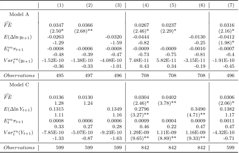
irra-Table 9: Irrationality and excess sensitivity. Subjective expectations on next year income level. Expectations calculated assuming a beta distribution function.

(1) (2) (3) (4) (5) (6) (7) Model A

d

F E 0.0347 0.0366 0.0267 0.0237 0.0316 (2.50* (2.68)** (2.46)* (2.29)* (2.16)*

E(∆lnyt+1) -0.0263 -0.0320 -0.0444 -0.0130 -0.0412

-1.29 -1.59 -0.82 -0.25 (1.98)*

Esu

t πt+1 -0.0008 -0.0006 -0.0008 -0.0009 -0.0009 -0.0010 -0.0007

-0.48 -0.39 -0.47 -0.73 -0.75 -0.81 -0.4

V arsu

t (yt+1) -1.52E-10 -1.38E-10 -4.08E-10 7.48E-11 5.82E-11 -3.15E-11 -1.91E-10

-0.36 -0.33 -1.01 0.43 0.34 -0.19 -0.45

Observations 495 497 496 708 708 708 496

Model C

d

F E 0.0136 0.0130 0.0304 0.0402 0.0306 1.28 1.24 (2.46)* (3.78)** (2.06)*

E(∆lnYt+1) 0.1315 0.1349 0.2796 0.3490 0.1382

1.11 1.16 (3.27)** (4.71)** 1.17

Esu

t πt+1 0.0008 0.0006 0.0006 0.0009 0.0004 0.0009 0.0011

0.33 0.27 0.28 0.46 0.22 0.47 0.47

V arsu

t (Yt+1) -7.85E-10 -5.07E-10 -9.23E-10 1.29E-09 1.11E-09 1.16E-09 -4.32E-10

-1.33 -0.87 -1.63 (9.65)** (8.89)** (9.33)** -0.71

Observations 599 599 599 842 842 842 599

Notes: Models (1)-(3): forecast errors and predictable income growth instrumented with the large set of instruments. Models (4)-(6): forecast errors and predictable income growth instrumented with the small set of instruments. Model (7): forecast errors instrumented with the small set of instruments and predictable income growth instrumented with the large set of instruments. In Model A, forecast errors are defined as the difference between the self reported income realizations, calculated as the midpoints of the reported intervals, at time t+ 1 and the subjective mean of next year’s family income level at timetcalculated assuming a beta distribution function. In Model C, forecast errors are computed as the difference between family income realizations from self reported income growth rates and subjective family income expectations. t-statistics in parentheses and *P <0.05 and **P <0.01.

tionality or partially the effect of irrationality. Hence, not taking into account irrationality may give biased evidence in favor of liquidity constraints. This conjecture is supported by results from model C. In columns 4 through 6 we use the smaller set of instruments, and

confirm the previously stressed results. Column 7 reports results when predictable forecast errors were obtained from the smaller set of instruments and predictable changes in income

were obtained from the larger set of instruments. In this last case the hypothesis that irrationality is a distinct and statistically significant component in explaining consumption

changes is confirmed.

One final remark on sample composition should be done. Because of the way we have built up consumption, starting from those who declared to have put money aside in the last

been selected against liquidity constraint families. Hence reported evidence from Table 9 could be biased in favor of our model. In particular, estimated coefficients of the predictable

changes in income and that of the subjective variance, between the others, could be biased and not statistically significant.

To avoid the selection problem we have decided to include in the sample also the re-spondents that declared that they have not been able to put money aside during last 12 months. For those respondents saving has been considered equal to 0. Under this

alterna-tive specification of consumption, the available observations have grown up to 717 (models (1)-(3) and (7)) and 1017 (models (4)-(6)) for model A and 817 (models (1)-(3) and (7)) and

1138 (models (4)-(6)) for model C. Results remains in line with those presented in Table 9. Estimated coefficients on predictable forecast error are a little smaller but significant in all the alternative specification of the empirical model. Thus confirming our previous

results. Moreover, and more importantly for the sample selection issue, also the coefficients on predictable income growth get smaller (to values around a half of those presented in

Table 9) and continue to be significant only in the same specifications they were in the original sample (model C under the specification (4)-(6)). Estimated coefficients for the

subjective variance term are in line with those in Table 9. This all confirming that our results are not induced by sample selection.11

7

Conclusions

We have presented evidence that suggests that anomalies in consumption, here the fact

that consumption reacts to predictable changes in income, can be explained by a behavioral model in which agents do not have rational expectations and make predictable errors in

forecasting income. We have tested and rejected the null of rational expectation.

This adds to the literature on testing rational expectations with self reported expec-tations, because we have demonstrated a connection between predictable forecast errors

and actual economic behavior. It is often argued that earlier contributions do not sup-ply evidence to support the claim that the elicited expectations really correspond to those

affecting the agent’s behavior. Our result that it is possible to partially explain agents consumption decisions using predictable forecast errors should therefore be of interest.

Moreover, we find that irrationality is an important and autonomous source of the excess

sensitivity of consumption, even when precautionary savings and liquidity constraints are

References

Attanasio O., (1998). A Cohort Analysis of Saving Behavior by U:S: Households. Journal

of Human Resources, 33, 575-609.

Browning, M. and A. Lusardi, (1996). Household Saving: Micro Theories and Micro Facts.

Journal of Economic Literature, 34, 1797-1855.

Carroll, C. D., (1992). The Buffer-Stock Theory of Saving: Some Macroeconomic Evidence.

Brookings Papers on Economic Activity, 2, 61-156.

Chamberlain, G., (1984). Panel Data. In Zvi Griliches and Michael D. Intrilligator, eds.

Handbook of Econometrics, Vol. II, Amsterdam: North-Holland, 1247-1318.

Das, M., and B. Donkers, (1999). How Certain are Dutch Households about Future

In-come? An Empirical Analysis. The Review of Income and Wealth, 45, 325-38.

Dominitz, J. (1998). Earnings Expectations, Revisions, and Realizations. Review of Eco-nomics and Statistics,80 ,374-388.

Dominitz, J. (2001). Estimation of Income Expectations Models Using Expectations and Realization Data. Journal of Econometrics, 102, 165-95.

Dominitz, J., and C. Manski. (1997). Using Expectations Data to Study Subjective Income Expectations. Journal of the American Statistical Association, 92, 855-867.

Flavin M., (1991). The Joint Consumption/Asset Demand Decision: A Case Study in

Robust Estimation. NBER Working Paper, 3802.

Flavin M. (1999). Robust Estimation of the Joint Consumption/Asset Demand Decision.

NBER Working Paper, 7011.

Giamboni, L. (2004). Do Husbands’ and Wives’ Predictions Irrationally Diverge?.CEIS

working paper, 203.

Hall, R., (1978). Stochastic Implications of the Life Cycle-Permanent Income Hypothesis: Theory and Evidence. Journal of Political Economy, 86, 971-87.

Hall, R., and F. Mishkin. (1982). The sensitivity of Consumption to Transitory Income: Estimates from Panel Data on Households. Econometrica, 50, 461-77.

Jappelli, T. and L. Pistaferri. (2000). Using Subjective Income Expectations to test for Excess Sensitivity of Consumption to Predicted Income Growth. European Economic

Re-view, 44, 337-58.

Ludvigson, M. and Paxson, C., (2001). Approximation Bias in Linearized Euler Equations.

Review of Economics and Statistics, 83, 242-56.

Muth, F., (1961). Rational Expectations and the Theory of Price Movements. Economet-rica, 29, 315-35.

Zeldes, S., (1989). Optimal Consumption with Stochastic Income: Deviations from