http://dx.doi.org/10.4236/ojps.2014.42006
How to cite this paper:Liu, F. C. S. (2014). Using Multiple Imputation for Vote Choice Data: A Comparison across Multiple Imputation Tools. Open Journal of Political Science, 4, 39-46. http://dx.doi.org/10.4236/ojps.2014.42006
Using Multiple Imputation for Vote Choice
Data: A Comparison across Multiple
Imputation Tools
Frank C. S. Liu
Institute of Political Science, National Sun Yat-Sen University, Kaohsiung, Taiwan Email: [email protected]
Received 30 December 2013; revised 3 February 2014; accepted 19 February 2014
Copyright © 2014 by author and Scientific Research Publishing Inc.
This work is licensed under the Creative Commons Attribution International License (CC BY).
http://creativecommons.org/licenses/by/4.0/
Abstract
One commonly acknowledged challenge in polls or surveys is item non-response, i.e., a significant proportion of respondents conceal their preferences about particular questions. This paper ap- plies the multiple imputation (MI) method to reconstruct the distribution of vote choice in the sample. Vote choice is one of most important dependent variables in political science studies. This paper shows how the MI procedure in general facilitates the work of reconstructing the distribu- tion of a targeted variable. Particularly, it shows how MI can be applied to point-estimation in de- scriptive statistics. The three packages of R, AmeliaII, MICE, and mi, are employed for this project. The findings, based on a Taiwan Election and Democratization Study (TEDS) samples collected af- ter the 2012 presidential election (N = 1826) suggest the following: First, there is little adjustment done given the MI methods; Second, the three tools based on two algorithms lead to similar results, while Amelia II and MICE perform better. Although the results are not striking, the implications of these findings are worthy of discussion.
Keywords
Multiple Imputation, Survey Research Methods, Item-Non-Response, Missing Values
1. Introduction
40
non-response data result in a biased proportion for interested variables (Bernhagen & Marsh, 2007). This paper attempts to apply multiple imputation (MI) in order to improve electoral forecasts. The findings echo the find- ings of other similar studies and argues that MI is a cost-efficient and methodologically sound approach which leads to better use of raw survey and poll data (e.g., Barzi, 2004. For a summary of other approaches for dealing with item-non-response problems, see Florez-Lopez, 2010)1. In addition to demonstration about how this MI approach helps solve the item-non-response problem, this paper compares three MI tool utilities: Amellia II, MICE, and mi.
2. Multiple Imputation for Electoral Studies with Missing Values
Multiple imputation (MI) refers to a technique by which researchers replace missing or deficient values with a number of alternative values representing a distribution of possibilities (Paul, Mason, McCaffrey, & Fox, 2008; Rubin, 1987)2. MI has been widely adopted for regression analysis. Researchers draw auxiliary variables, those related to a target variable of interest, from theories and the literature, and then use MI algorithm or software to generate values for each missing value based on the distributions of selected auxiliary variables. This procedure will create a number of supplemental data sets in which all missing values are filled. To obtain unbiased and ro-bust regression coefficients, the researcher first runs models based on every data set generated from the above procedure. This is followed by averaging the coefficients and standard errors across the models (King, Honaker, Joseph, & Scheve, 2001; Snijders & Bosker, 2011; Stuart, Azur, Frangakis, & Leaf, 2009)3.
Electoral scholars have started paying attention to the MI approach and applying it to electoral forecasts. Bernaards et al. (2003), for example, compares descriptive statistics for data drawn from the MI procedure to determine if two or more methods generate similar results. Bernhagen and Marsh (2007) adopt this approach by treating non-voters and non-party identifiers as missing and recreate “hypothetical (100% turnout)” votes for in-dividual elections and inin-dividual parties. Although their works use conventional MI methods to study the rela-tionship between explanatory variables and a chosen response variable, they also suggest that using MI to study a chosen response variable is one way to understand an electorate. That is, scholars can pay more attention to advancing the accuracy of descriptive statistics from dependent variable than explaining the variance of the re-sponse variable. Although this novel focus is absent from Rubin(1987), there is little methodological reason to object to the scholarly action of imputing the targeted response variable or dependent variable; instead, studying the vote choices of non-voters was proposed at the time MI was introduced to the discipline (King, Honaker, Joseph, & Scheve, 2001; Snijders & Bosker, 2011). G. David Garson supports this perspective as well: “for purposes of univariate analysis (e.g., understanding the frequency distribution of how subjects respond to an opinion item) imputation can reduce bias and often is used for this purpose if data are missing at random.”4
3. The Dataset
Taiwan’s Election and Democratization Study for the 2012 presidential elections (TEDS2012P, N = 1826) is used to examine the applicability of the MI method5. The TEDS2012P data was collected during mid-January and early March of 2012 (the Election Day is on January 14, 2012). The data set was weighted using raking in
1Allison (2001) holds the conventional view that when it comes to linear regression, list-wise deletion is the least problematic, and a safer
method, for dealing with missing data. This paper focuses on advancing the accuracy of the proportion of dependent variables such as voter turnout, vote choice, etc., and is not devoted to the debate about the choice of approach.
2
MI is a method commonly used to deal with missing data problems, including item-nonresponse (nonresponse to some, but not all, survey questions) and unit-nonresponse (nonresponse to all survey questions). A common and still useful alternative is list-wise deletion of obser- vations due to both item-nonresponse and unit-nonresponse in the regression analysis. However, because a significant number of observa- tions are excluded from analysis, this method may yield biased parameter estimates. While the default procedure of most statistical packages
excludes the observations with missing values, list-wise deletion has been identified as a problem for most electoral studies (Gelman, King,
& Liu, 1998). This concern regarding biased estimates can be minimized if the loss of cases due to missing data is less than about 5%, and if
pretest variables can reasonably be included in the models as covariates (Graham, 2009).
3While some scholars may think this technique is unrealistic, or have concerns about “making up” data, we need to acknowledge that
“com-plete-case analyses require [even] stronger assumptions than does imputation” (Stuart, Azur, Frangakis, & Leaf, 2009: p. 1134).
4See http://faculty.chass.ncsu.edu/garson/PA765/missing.htm
5Data analyzed in this paper were from Taiwan’s Election and Democratization Studies, 2012: Presidential and Legislative Elections (TEDS
2012) (NSC100-2420-H-002-030). The coordinator of multi-year project TEDS is Professor Yun-Han Chu (National Taiwan University).
The principal investigator is Professor Chi Huang. More information is available on TEDS website (http://www.tedsnet.org). The author
41
order to meet the population attributes characterized by the following variables published in 2011: gender, age (five levels), education (five levels), and region (six areas of Taiwan). In this investigation, the respondents were asked about whether they turned out to vote and what their voting choices were.
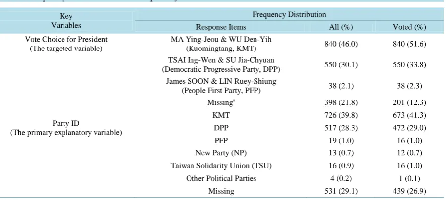
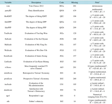
As the base for calculating vote share of each team of candidates, a subset data forTEDS2012Pis created to include only those who voted (N = 1629)6. As Table 1 shows, in this subset the missing rate for vote choice, the targeted variable, is 12.3%; that is, 201 out of 1629 respondents said they voted but did not reveal which presi-dential candidate they voted for. Note that instead of using all of the more than 150 variables from TEDS2012 for this study, I selected variables and made a list of those that I expected to be related to vote choice, as detailed in Table 2. A number of explanatory variables for partisanship are needed because the question of party identi- fication itself has a high level of missing values (26.9%). This situation is common in Taiwan surveys because a growing number of voters are either ambivalent about the parties or aware of the negative effects of partisan la- bels in their daily lives. This fact suggests that we cannot simply use the party identification variable to predict voter choice.
4. Software Packages for the MI Analysis: Amelia II, MICE, and MI
A growing number of researchers in academic and commercial institutes choose the multi-platform statistical language R7. Within the Comprehensive R Archive Network (CRAN) there are a number of packages associated with MI. The three packages chosen for this study are Amelia II, MICE, and mi.
[image:3.595.91.541.435.637.2]Amelia II is a cross-operation system package designed to process the Expectation Maximization with impor-tance re-sampling (EMis) algorithm, one of the suggested algorithms using Markov chain Monte Carlo (MCMC) methods to calculate imputed values (Honaker, King, & Blackwell, 2009, 2011). Expectation Maximization (EM) is also called “joined modeling” (JM), “specifying a multivariate distribution for the missing data, and drawing imputation from their conditional distributions by MCMC techniques” (Buuren & Groothuis-Oud- shoorn, 2011: pp. 1-2). Amelia II is characterized by its speed using EMis and a handy graphical user interface (GUI), allowing the researcher to manage types of variables by simply designating them as nominal or ordinal variables. After variables are specified, it automatically transforms nominal variables into dummy variables and regards them as categorical variables during the imputation process8.
Table 1.Frequency distribution of the two primary variables.
Key Variables
Frequency Distribution
Response Items All (%) Voted (%)
Vote Choice for President (The targeted variable)
MA Ying-Jeou & WU Den-Yih
(Kuomingtang, KMT) 840 (46.0) 840 (51.6)
TSAI Ing-Wen & SU Jia-Chyuan
(Democratic Progressive Party, DPP) 550 (30.1) 550 (33.8)
James SOON & LIN Ruey-Shiung
(People First Party, PFP) 38 (2.1) 38 (2.3)
Missinga 398 (21.8) 201 (12.3)
Party ID
(The primary explanatory variable)
KMT 726 (39.8) 673 (41.3)
DPP 517 (28.3) 472 (29.0)
PFP 19 (1.0) 16 (1.0)
New Party (NP) 13 (0.7) 12 (0.7)
Taiwan Solidarity Union (TSU) 16 (0.9) 16 (1.0)
Other Political Parties 4 (0.2) 1 (0.1)
Missing 531 (29.1) 439 (26.9)
Source: TEDS2012P; N = 1826b; a“missing” includes “refuse to answer”, “don’t know,” and “skip”. bThe total N include 1629 who turned out to vote, 194 who did not vote, and 3 gave no response.
6Note that the turnout rate calculated based on TEDS2012 is 89.36% (1629/1862), which is much higher than the real figure 74.38%.
7Besides R, commercial packages such as SAS, SPSS and STATA also support MI procedure. For example, an illustration of using STATA
for MI can be found: http://www.stata.com/meeting/spain12/abstracts/materials/Escobar_Jaime.pdf.
8For researchers following the three-step procedure of conducting MI, Zelig, another package compatible with R, is suggested for the
com-bination stage (Imai, King, & Lau, 2004). Since hypothesis testing is not the goal of the present study, the analysis below will concentrate on
42
Table 2.List of variables used for imputing vote choice.
Variable Description Code Missing Notea
vote Vote Choice 2012 H01a 201 dichotomous
partyID Party Identification Q01b 439 multinomial;
X2 = 930.7, df = 5
likeKMT The degree of liking KMT Q02 106 a 11-point scale;
X2 = 613.1, df = 20
likeDPP The degree of liking DPP Q02a 122 a 11-point scale;
X2 = 598.0, df = 20
likePFP The degree of liking PFP Q02b 209 a 11-point scale;
X2 = 33.0, df = 20
TsaiScale Evaluation of Tsai Ing-Wen J02a 120 a 11-point scale;
X2 = 663.8, df = 20
SuScale Evaluation of Su Jia-Chyuan J02b 168 a 11-point scale;
X2 = 649.9, df = 20
MaScale Evaluation of Ma Ying-Jio J02c 107 a 11-point scale;
X2 = 702.2, df = 20
WuScale Evaluation of Wu Den-Yih J02d 132 a 11-point scale;
X2 = 628.5, df = 20
SoonScale Evaluation of James Soong J02e 157 a 11-point scale;
X2 = 92.4, df = 20
LinScale Evaluation of Lin Ryue-Shiung J02f 303 a 11-point scale;
X2 = 82.74, df = 20
tvNews Most frequently watched TV
news Channel A03 201
10 types (multinomial)b;
X2 = 425.65, df = 18
retroEcon Retrospective Taiwan’ Economy E01 46 3-option multinomial;
X2 = 219.8, df = 4
prosEcon Prospective Taiwan’s Economy E02 260 3-option mutinomial;
X2 = 189.8, df = 2
incScale Evaluation of the
Ma administration C01 105
a 4-point ordianl ;
X2 = 545.0, df = 6
demScore Satisfaction with
Taiwan’s Democracy F05 78
a 4-point ordinal;
X2 = 116.0, df = 6
age1 Respondent’s age S01 0 Numerical
(ranging from 20 to 91)
eth Father’s ethnicity S02 16 6 types (multinomial);
X2 = 128.8, df = 10
Source: TEDS2012; N = 1629; a. X2 test of independence against “vote”; the variables listed here are correlated with “vote” at least to the 0.05 signi-ficance level; b. In tvNews top ten most watched TV news channels are coded to 1 to 10, respectively; other channels are coded into 11; 0 is used for those saying they never watch TV news; c. Education level that is found significantly related to vote choice using the 2008 presidential election data is not found in this study using TEDS2012 and, thus, it is dropped from the variable list.
43
The package mi uses a strategy similar to MICE: proceeding one-variable-at-a-time. It starts with me-dian/mode for missing data, conducts a specified number of iterations, and cycles through until convergence occurs. It then draws a bootstrap sample to create imputed values. What distinguishes mi from MICE is that mi adds algorithms related to semi-continuous data (such as age) and adds Bayesian models to assist researchers in conducting more stable estimates of imputation models (Su, Gelman, Hill, & Yajima, 2011).
He and Raghunathan (2009) conduct a series of experiments and compare the performance of MI using se-quential regression, i.e., chain equations. They find that all methods using chain equations perform well for es-timating the marginal mean and proportion, as well as regression coefficients, even when the error distribution is non-normal. However, they warn that the MI results can be very biased when error distributions have extremely heavy tails, i.e., when data includes extreme values.
As King, Honaker, Joseph, and Scheve (2001) argue, EM is a faster and less complex alternative to IP. Con-cerned about the fact that EM algorithm ignores estimation of uncertainty, however, they propose EM with im-portance re-sampling (EMis) to solve the uncertainty problem in EM. This implies that Amelia handles the MI issues more efficiently than MICE and mi. They believe the algorithms will frequently draw an estimated mean and variance from the disputed data sets created from entire multivariate models of observed data posterior through IP use. In order to obtain the specific result expected, a substantial amount of time may be devoted to drawing before convergence occurs. This study confirms this argument, and it will discuss in the findings section.
5. Experiment Design
The chosen target variable of this study is vote choice, and the explanatory variables chosen are those theoreti-cally related to vote choice. The partisanship-related explanatory variables are shown in Table 2. These va-riables include respondent’s party identification, their evaluation of the three major political parties that have named candidates,9 the evaluation of the candidates, the evaluation of the incumbent president’s administration, the ethnicity of the respondent’s father, and age. These variables are found theoretically and empircally related to vote choice (Liu, 2010). For example, age is considered because it is found that young voters favor DPP can-didates over that of the KMT. As the behavior of watching TV news in Taiwan can reveal one’s partisan orien-tation, it is also included as an imputation variable. I also employed some other variables that may not seem di-rectly related to one’s partisanship, include a prospective and retrospective evaluation of Taiwan’s economy, and an evaluation of Taiwan’s democracy. However, these are statistically related to vote choiceto at least the 0.05 level ina Chi-square test.
To proceed to conduct analysis using MI and related tools, I assume that the missingness pattern of TEDS 2012 is missing at random (MAR)10. A data set X for MI, composed of the variables listed in Table 2, was created (N = 1629). The respondents in this data set are those who turned out to vote. Each of the three R pack-ages was used to create 10 imputed data sets. The vote share of each data set was then computed. After this, the means of deviation for the 10 vote shares was calculated. These results will be compared to the vote share cal-culated based on data set X and real election results.
6. Findings
As published in January 14, 2012, the vote shares for Ma Ying-Jeou and Wu Den-Yih (Kuomingtang or KMT president and vice president candidates), Tsai Ing-Wen and Su Jia-Chyuan (Democratic Progressive Party or DPP candidates), James Soon & Lin Ruey-Shiung (People First Party or PFP candidates) were 51.60%, 45.63%, and 2.76%, respectively11. The vote choice distribution derived from TEDS2012P (N = 1629), however, is quite biased toward KMT candidates Ma and Wu (58.82%); the sample also underestimates the vote share for the DPP’s Tsai and Su (38.52%).
9Note that I use PFP as a convenient label for the independent candidates Soong and Lin. They are seen as representatives or nominees for
the PFP as Soong is the party chair. However, they ran as independent candidates.
10Missingness at random (MAR) is a commonly held assumption about the missing patterns of original data, meaning the chosen
missing-ness indicators are independent of the unobserved data. According to Snijders and Bosker (2011) it is recommended “to collect auxiliary
da-ta that is predictive of missingness indicators and of the values of unobserved dada-ta points. Including such auxiliary dada-ta can push the design in the direction of MAR” (p. 150). The other two assumptions about the pattern of missingness are Missingness completely at random (MCAR) and Missingness not at random (MNAR). MCAR means that the missingness indicators are independent of the complete data; MNAR is a situation where missingness is not at random and will always depend on untestable assumptions. MNAR and will be more com-plicated and leave open more questions than the MAR case.
44
Given this scenario, I originally expected that MI could assist researchers in adjusting the sample distribution. This is the case, as is shown in Table 3. However, it does not perform as well as I had expected: no matter which package was used—Amelia, MICE, or mi, the extent to which MI corrects the distribution is very limited, although the direction of adjustment is correct. First, the point estimate of vote share for the KMT’s Ma & Wu was correctly lowered down by about 2%, while, for the DPP’s Tsai & Su, the figure was correctly raised by about 1%. Second, the vote share of PFP’s Soong & Lin was over estimated by almost 1%. The difference be-tween the DPP and KMT in actual vote share is 5.97%. If we simply use TEDS2012Pfor electoral prediction, the data would lead us to expect that the KMT’s vote share is 20.3% over the DPP’s. The MI methods effectively help narrow the gap between the point estimate derived from the sample and real election results mildly to 17.33% (Amelia II), 17.15% (MICE), and 18.62 (mi) but the magnitude of adjustment is not striking. The distribution of vote choice after adjustment remains biased toward KMT’s Ma & Wu.
Next, it is found that the results derived from the two competing MI methodologies, i.e., joint modeling (Amelia) and chained equations (MICE and mi) are similar. The averages for vote shares drawn from 10 impu-tation data sets using each of the R packages are about the same. Even so, I find Amelia and MICE are more ef-ficient than mi in terms of computing speed, while Amelia is superior to MICE and mi regarding point estima-tion12.
I then use the 10 imputed data sets created by Amelia II to examine the distribution of vote choice for the 201 respondents who turned out to vote but did not reveal their vote choices in the TEDS survey. The calculation of the average suggests that 43.63% (sd = 15.53) are likely to be the supporters of DPP’s Tsai & Su, 39.55% (sd = 14.50) are likely to be KMT’s Ma & Wu supporters, and 6.82% (sd = 2.76) may have voted for Soong & Lin. This result suggests a pattern that may not change the overall distribution of vote choice much when the imputed answers for these respondents are added back to the data set X.
7. Conclusion
Analyzing survey data is one of the most promising methods for forecasting election results. A commonly per- ceived problem for forecasting with raw data is that a significant proportion of respondents conceal their prefe- rences. This is particularly a problem in Taiwan when surveys ask sensitive questions, or when it asks about po- litical preferences during the campaign season. Hence, the true distribution of vote choices remains a black box and prediction based on raw data and simply ignoring item-nonresponse respondents can be biased, if not mis- leading.
This study contributes to this stream of research by providing a more solid research design by taking voter
Table 3.Comparison of MI results across Amelia II, MICE, and MI.
Election Results
MI Methodsb
Vote Share %a
Ma & Wu (KMT)
Tsai & Su (DPP)
Soong & Lin (PFP)
Real election results 51.60 45.63 2.76
Raw data (before using MI) 58.82 38.52 2.66
Amelia II 56.96
(0.025)
39.63 (0.002)
3.41 (0.025)
MICE 56.86
(0.034)
39.71 (0.003)
3.43 (0.016)
MI 58.02
(0.034)
39.58 (0.003)
2.40 (0.006)
Source: TEDS 2012; a. The vote share (mean) and standard deviations shown in parentheses are calculated based on the 10 data sets generated from the MI procedure; b. The same seed 123 was used and the number of data set to create is set to 10.
12Amelia remains a more efficient choice as the chained equations take much more time to reach the convergence stage than Amelia. When
using MI, I first encountered the problem of reaching convergence after 3 hours of calculation (compared to Amelia’s 3 minutes and Mice’s 5 minutes). After removing “partyID”, which has 26.9% missing (this can make it difficult to converge given information drawn from other variables), it took about 15 minutes (17 iterations) for convergence to occur. For the comparison about regression coefficients using the four MI packages, including Amelia, MICE, mi, and aregImpute, see
http://pj.freefaculty.org/guides/Rcourse/multipleImputation/multipleImputation-1-lecture.pdf, which suggests that there is little difference
45
turnout into consideration, calculating vote shares based on those who did turn out to vote. It also and provides a comparison across MI tools. In sum, the findings suggest the following. First, MI has the leverage to adjust bi-ased vote share and does not make predictions less accurate. Second, it is likely that the sample for TEDS2012P overly represents KMT supporters. Third, there is little to worry about concerning which kind of MI algorithms to use since, when it comes to point estimation, they all perform well. The three MI packages Amelia II, MICE, and mi produce similar results in terms of predicting vote choice. This pattern echoes the literature stating that the employment of the MI approach does not lead to less accurate results than if nothing had been done.
The results for MI adjustment are not as striking, as I originally expected predicted in the initial stages of this study. That is, none of the three packages adjusted the predicted vote share to a satisfactory level that approx-imates the election result. If there is nothing wrong with the MI method, or the three R packages, there is room to consider alternative explanations, particularly in the sample itself.
What if the TEDS2012P falls short of representing the electoral body? As a post-electoral face-to-face survey data set drawn from the population based on geology and demographics, it is possible that such a sample may not be the same as one based on political ideology. In other words, when it comes to predicting election results, this sample may fall short of mirroring the unknown distribution of voters’ party identification. Additionally, it cannot avoid substantial structural bias caused by conventional types of errors such as systematic non-response errors, sampling errors, and frame errors. This means a sample collected at a specific will fail to encompass cer-tain elements of the target population.
Coverage error is the most important form of frame error and it is very likely to be the cause of biased sam-pling. “Coverage error” includes under coverage, over coverage, and duplicated listings. In this study, it is found that KMT supporters can be over covered either at the sampling or the interviewing stage. Therefore, theoreti-cally, it is important to examine and understand the sampling process and the causes of the bias in terms of par-tisanship. Practically, it is difficult to do so, because, in Taiwan, no one has the authority or legal right to double check with the 201 respondents who hided their vote choices in the TEDS2012 survey for their true preferences. Therefore, this line of study will progress only if the respondents allow the researcher to check their untold pre-ferences. This requires a new research design in which researchers themselves collect datas. Given a panel data, or the ability to conduct follow-up interviews, future studies would be able to conduct conduct external validity checks for guesses generated by MI.
From here, I expect two topics to be addressed in future research. The first is the external validation of the MI method, i.e., comparing imputed values with true preferences. The application of MI to forecasting electoral re-sults requires a more solid grounding for external validity checks. Second is exploring the methods and tools for diagnosing the missingness patterns. In this study, I adopted the conventional assumption that the missingness of a targeted variable is missing at random (MAR). We should keep in mind what Paul Allison (2001) has warned: “Other multiple imputation methods that make less restrictive distributional assumptions are currently under development, but they have not yet reached a level of theoretical or computational refinement that would justify widespread use” (p. 85). Whenever there are tools and methods available for researchers to examine the pattern of missingness, it should be taken as a priority in moving the discipline forward.
Acknowledgements
This study is particularly supported by “Aim for the Top University Plan” of the National Sun Yat-sen Univer-sity and MOST (101-2410-H-110-041-SS3). The author thanks the reviewers for comments.
References
Allison, P. D. (2001). Missing Data. London: Sage Publications, Inc.
Barzi, F. (2004). Imputations of Missing Values in Practice: Results from Imputations of Serum Cholesterol in 28 Cohort Studies. American Journal of Epidemiology, 160, 34-45. http://dx.doi.org/10.1093/aje/kwh175
Bernaards, C. A., Farmer, M. M., Qi, K., Dulai, G. S., Ganz, P. A., & Kahn, K. L. (2003). Comparison of Two Multiple Im- putation Procedures in a Cancer Screening Survey. Journal of Data Science, 1, 293-312.
Bernhagen, P., & Marsh, M. (2007). The Partisan Effects of Low Turnout: Analyzing Vote Abstention as a Missing Data Problem. Electoral Studies, 26, 548-560. http://dx.doi.org/10.1016/j.electstud.2006.10.002
46
http://dx.doi.org/10.1057/jors.2009.66
Gelman, A., King, G., & Liu, C. (1998). Not Asked and Not Answered: Multiple Imputation for Multiple Surveys. Journal of the American Statistical Association, 93, 846-857. http://dx.doi.org/10.1080/01621459.1998.10473737
Graham, J. W. (2009). Missing Data Analysis: Making It Work in the Real World. Annual Review of Psychology, 60, 549- 576. http://dx.doi.org/10.1146/annurev.psych.58.110405.085530
He, Y., & Raghunathan, T. E. (2009). On the Performance of Sequential Regression Multiple Imputation Methods with Non- Normal Error Distributions. Communications in Statistics-Simulation and Computation, 38, 856-883.
http://dx.doi.org/10.1080/03610910802677191
Honaker, J., King, G., & Blackwell, M. (2009). Amelia Software Web Site http://gking.harvard.edu/amelia
Honaker, J., King, G., & Blackwell, M. (2011). Amelia II: A Program for Missing Data. Journal of Statistical Software, 45,
1-47.
Imai, K., King, G., & Lau, O. (2004). Zelig: Everyone’s Statistical Software. http://GKing.Harvard.Edu/zelig
King, G., Honaker, J., Joseph, A., & Scheve, K. (2001). Analyzing Incomplete Political Science Data: An Alternative Algo- rithm for Multiple Imputation. American Political Science Review, 95, 49-69.
Liu, F. C.-S. (2010). Reconstruct Partisan Support Distribution with Multiply Imputed Survey Data: A Case Study of Tai-wan’s 2008 Presidential Election. Survey Research, 24, 135-162.
Paul, C., Mason, W. M., McCaffrey, D., & Fox, S. A. (2008). A Cautionary Case Study of Approaches to the Treatment of Missing Data. Statistical Methods and Applications, 17, 351-372. http://dx.doi.org/10.1007/s10260-007-0090-4
Rubin, D. B. (1987). Multiple Imputation for Nonresponse in Surveys. Wiley Series in Probability and Mathematical Statis- tics. Applied Probability and Statistics. New York: Wiley. http://dx.doi.org/10.1002/9780470316696
Snijders, T. A. B., & Bosker, R. (2011). Multilevel Analysis: An Introduction to Basic and Advanced Multilevel Modeling
(2nd ed.). Longdon: Sage Publications Ltd.
Stuart, E. A., Azur, M., Frangakis, C., & Leaf, P. (2009). Multiple Imputation with Large Data Sets: A Case Study of the Children’s Mental Health Initiative. American Journal of Epidemiology, 169, 1133-1139.
http://dx.doi.org/10.1093/aje/kwp026
Su, Y.-S., Gelman, A., Hill, J., & Yajima, M. (2011). Multiple Imputation with Diagnostics (mi) in R: Opening Windows into the Black Box. Journal of Statistical Software, 45, 1-31.