Divorce and the Option Value of Marital Search

Munich Personal RePEc Archive

Divorce and the Option Value of Marital

Search

Filoso, Valerio

Department of Economic Theory and Applications, University of

Naples “Federico II”, Italy, and CHILD (Centre for Household,

Income, Labour and Demographic economics), Turin, Italy

22 February 2007

Online at

https://mpra.ub.uni-muenchen.de/2038/

Economic Growth: Institutional and Social Dynamics

WORKING PAPER SERIES

Divorce and the Option Value of Marital Search

Valerio Filoso

Working Paper 015

March 2007

Divorce and the Option Value of Marital Search

Valerio Filoso Working Paper 015

Abstract - This works tests whether or not the introduction of divorce law changes the timing of marital search. Common sense suggests that rational agents should adjust to the divorce risk by increasing the average length of search spell, whereas the option value theory stresses the role played by irreversible investments: in this case, the new exit option available to married partners should result in shorter search spells. Using a dynamic model of marital search, a new dataset of retrospective individual Italian data, and two robust statistical specifications based upon the Before-After estimator, we find strong evidence that the legal innovation actually lowered the age at marriage, thereby worsening the level of marital matching, and possibly reinforcing self-fulfilling prophecies of divorce.

JEL CODES:J12, C41, D83

KEYWORDS:Marital Search, Divorce, Marriage

The author thanks Yoram Weiss, Manuel Trajtenberg, Yona Rubinstein, Avi Tillman, and Ori Zax at Tel Aviv University. Thanks also to Myoung-Jae Lee and Etta Chiuri. Erasmo Papagni has provided great suggestions and enduring support. All errors are mine.

1. INTRODUCTION

If I am not for myself, who will be for me? And if I am only for myself, what am I? And if not now, when?

Pirqe Avot, 1:14.

1

Introduction

From the economic point of view, marriage is a long-run contract which com-mands monogamy and couple-specific investments that are expected to increase the value of the union across time. When legal norms forbid divorce, the accu-mulation of marital human capital does not need to account for default risk. By contrast, when unilateral divorce is permitted, married individuals run the risk of the partner walking away. Should this occur, most couple-specific investments cannot be used without large switching costs over the next marriage. A common way to cover from such costs is to search harder and longer for matches which are less likely to dissolve. Thus, if legal norms make marriage a risky contract, rational agents should be very careful about the quality of their matching. Nev-ertheless, no-fault divorce also provides the opportunity to break unilaterally an unhappy marriage: this action prevents the risk of spending one’s life in distress and gloominess. By allowing for this exit option, the same rational agents may become less cautious when considering a marriageable mate and then could de-cide to stop their search at an earlier age. Whether age at marriage decreases or increases in response to the introduction of divorce is a matter of empirical investigation.

It is a controversial issue whether divorce laws change incentives to marry. Until now, economic debate on the effects of divorce law has focused mainly on changes from consensual to no-fault divorce legislation using aggregate state-level data for the US. The stream of literature which relates to Becker’s applica-tion of Coase’s theorem to family organizaapplica-tion (Gray, 1998; Peters, 1992, 1986) maintains that marital bargaining can offset legal innovations, while opponents (Friedberg, 1998; Allen, 1992) find that changes in legislation have a significant impact on divorce rates. Most recent approaches (Wolfers, 2006) find that the im-pact on divorce rates is only temporary, while in the long run the Coase theorem holds for married couples. The alternative approach based on collective models (Chiappori, Fortin, and Lacroix, 2002) has long stressed the role played by divorce laws in shifting bargaining positions within marriage. Recently, Allen, Pendakur, and Suen (2006) have estimated the effect on the age at marriage of a change from consensual to no-fault divorce legislation, controlling for state heterogeneity and time trends: results show a slight increase in the mean age at marriage and a 5% increase in its standard deviation for subjects living in states which adopted no-fault divorce. Basically, all previous literature is aimed at identifying the ef-fects of changes in existing divorce legislation, not the effect of ex novo divorce legislation.

1. INTRODUCTION

law in a social scenario in which marriage is not rescindable using a microeconomic model of optimal sequential search (Bougheas and Georgellis, 1999; Matsushita, 1989). The model is then estimated over a dataset of retrospective individual histories, using observations before and after the reform. In our view, the pro-cess of mutual search is lengthy, costly, and deeply interrelated with other crucial decisions in one’s life, such as the educational path or participation in the labor market. These dimensions are relevant since improving and refining personal traits – such as educational attainment, physical appearance, financial robustness – may increase the probability of finding and matching with better partners. Yet these actions are usually time-intensive and can be combined with marriage only at a substantial cost. This shows the emergence of a trade-off between the prob-ability of marriage and its timing, arising from strategic actions that boost one’s competitive position in the marriage market, which in turn contribute to post-pone the event of marriage itself. In this context of dynamic action, the notions of investment irreversibility and value of waiting (Dixit and Pindyck, 1994) play a key role. We test whether after the legal reform introducing divorce, marriage has become a less irreversible investment. If so, the option value of waiting for a better match should register a drop, resulting in shorter search spells for the representative agent. Moreover, the introduction of divorce has possibly affected the probability of marriage indirectly as well, through changes in choice variables like education and job status, provided that participants in the marriage market attach value to specific personal traits.

In the econometric section, two specifications, one parametric and another semiparametric, were estimated for the age at marriage on a panel of 5,814 Italian subjects. The legal regime change is modeled through a Before-After estimator (Lee, 2005; Heckman, LaLonde, and Smith, 1999): taking account of time trends and personal characteristics including education, job status, religious attendance, and family background, we find that divorce has strongly contributed to shorten the average search spell, mainly for women, possibly reinforcing self-fulfilling prophecies of divorce. Most likely, this differential result for gender specification depends upon the binding biological constraint that women have on fertility. Ed-ucational choices seem little influenced by divorce, both for women and men; on the contrary, the same law lowered women’s propensity to gain more stable jobs, while increasing the role played by men’s occupational status in determining age at marriage. Also, an educational level higher than similar individuals adversely affects the probability of marriage, but this peer effect is stronger for men. After divorce was passed, religiously committed people modified their search behav-ior: women shortened their search spells, while no significant effect is reported for men. Above all, the strongest effect of divorce reform appears to be a large decline in the value of marital search, a result which confirms the irreversibility hypothesis and the underlying theoretical model.

2. SOMESTYLIZEDFACTS

studies were started. Third, it is found that subjects under study behaved accord-ing to the standard predictions of option value theory.

The article proceeds as follows: the second section surveys basic facts about marriage in Italy and presents evidence of aggregate trends; the third section builds the dynamic model of marriage and divorce under the assumption of no-fault divorce; the fourth describes the details of variables included in the empir-ical model; the fifth discusses results from estimation; the sixth provides final comments and further developments.

2

Some Stylized Facts

A preliminary outlook at the data1from an aggregate point of view displays some major trends occurring in the Italian marriage market between 1950 and 2001. During the period under scrutiny two main legal innovations in marriage law took place. On 1st December 1970, following an ongoing European trend, the Italian Parliament passed a law permitting unilateral divorce: while marital sep-aration was already legally allowed, under the new regime, for the first time in Italian history, spouses were allowed to untie the marriage contract and possibly remarry after five years of legal separation. Four years later, a public consultation promoted by traditional Catholics and Conservatives for the abolition of the new law saw the anti-divorce coalition soundly defeated. This event testified to the changing view of marriage spreading through Italian society and an increasingly strong preference for more liberal customs. Finally, the five-years waiting time between separation and divorce was shortened to three years by a minor reform in 1987.

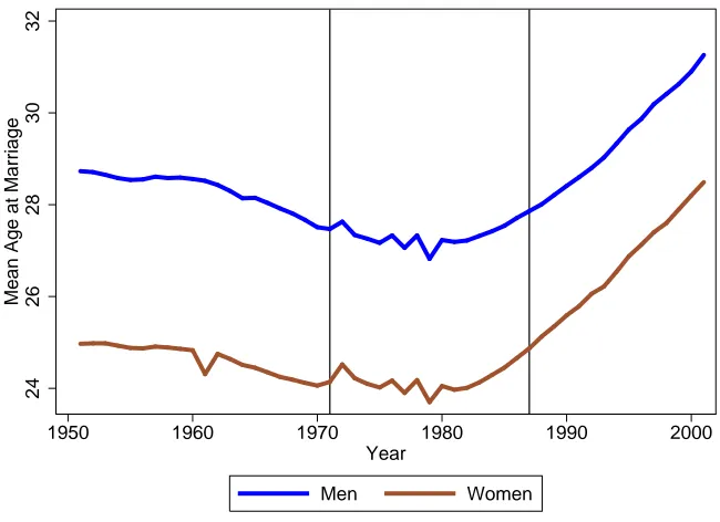
Over the years under study (1950–2001), thenuptiality rate(the total number of marriages, in a given year, divided by the total population between 16 and 49 years old), plotted in fig. 1, decreased from 14% to 10% .2 In the same period,

mean age at marriage increased for men from 28.9 to 31.26, whereas for women it recorded a striking increase from 24.97 to 28.49, as can be seen in fig. 2. Both graphs show two different temporal patterns for the two time series. Nuptial-ity rate shows a fairly steady downward trend starting shortly after 1960, with temporary reversal around 1971 and 1987: since the total number of marriages also includes second and subsequent marriages, the increased ratio accounts for those who were waiting to divorce and remarry. The graph of mean age at mar-riage does not show a similar neat trend; rather, it suggests a u-shaped curve with its lower bound around the period 1970–1980 and a steady increase until recent years. Whether or not the 1970 divorce reform played a role in determining age at marriage, its outcome was an increased variability of age at marriage, whereas the minor reform of 1987 does not seem not to affect the upward trend of the same variable.

The numbers for divorce and separation display the most striking evidence

1_{Evidence provided in this section and in the graphs section is taken from ISTAT (Italian}

Sta-tistical Institute) and represent the whole staSta-tistical universe.

2_{The United States experienced a decrease from 11.1% to 8.4% , the French crude marriage}

2. SOMESTYLIZEDFACTS

for changing behavior of Italian couples, as shown in fig. 3. In 1950, theseparation rate(the ratio between legal separations and new marriages in a given year) was 1.5%, while in 2001 the same ratio rocketed to 29.1%. During the period 1971– 2001, the divorce rate (the ratio between total divorces and new marriages in a given year) jumped from 4.2% to 16.7%.3

As a rule of thumb, the ratio between separations and marriages can be con-sidered an initial indicator of marital risk at an aggregate level. All caveats pro-vided, it can be affirmed that, without other a priori information, marriage is steadily becoming a riskier business. On the one hand, the observer could be tempted to establish a simple relationship between the increasing level of marital risk and the increasing age at marriage: since marriage is a long-run contract that calls for specific investments, an increase in the average level of risk could be at least partially offset by an increase in the quality of marriage, and then in the time spent in the search for a partner. However, this does not seem the case for Italy, given the rise in separation and divorce which occurred during the same period. On the other hand, a well-established empirical correlation in the literature on marriage breakup states that a higher age at marriage decreases the likelihood of divorce. Marriage surprises (Weiss and Willis, 1997), driven by financial and preference shocks that make marriage relationships unstable, are more likely to happen when spouses are young. However, aggregate Italian data show that age at marriageandmarital risk both registered a steady increase. This apparent con-tradiction might be explained if we assume that divorce follows an exogenous temporal path and age at marriage tries to catch up with it. In other words, peo-ple may try to compensate for the higher levels of riskiness by being increasingly selective in their search process. Alternatively, people could compensate the in-creased level of marital risk by being more prone to separation and divorce, there-fore investing less in marital capital and then reinforcing self-fulfilling prophecies of divorce.

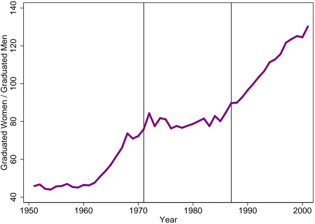
Matching choices are mainly influenced by educational choices, since school-ing and university attendance can be combined with marital life, pregnancies, and child rearing only at a substantial cost. This is not to say that highly edu-cated women are less likely to marry, just the opposite could be true. Investment in education is strategic not only in the labor market: as marriage becomes in-creasingly based on cooperation rather than traditional gender roles, more edu-cation can result in better matches. A striking trend of the increasing eduedu-cation of women is depicted in fig. 4, where the ratio of female to male university grad-uated is considered since it encompasses all completed levels of schooling. It was only 45.9% in 1950, while it almost completely reversed to 130.2% in 2001; the increasing trend was temporarily halted during the years 1970–1987, the same years in which the age at marriage appears almost stationary.

To sum up, in the period under study, nuptiality decreased steadily, while age at marriage rose, mainly due to higher levels of education; indicators of marital disruption reveal increasing risk in marriage, while women seem increasingly involved in higher education, compared to men. In the empirical section of the

3_{A caveat must be provided: the ratio between separations and divorces over marriages in the}

3. THEORETICALFRAMEWORK

paper, some of these trends are included in the regression model to evaluate the differential effect of the divorce law, holding other variables constant.

3

Theoretical Framework

The theoretical model used to explain the decision to marry is built around the assumption that the search process for a partner is costly and time-consuming. We explicitly endorse a search-theoretic structure resembling the one provided in Filoso (2005), albeit slightly simplified.

In this stylized framework, all agents live infinite lives and in each period receive a marriage proposal from an agent of the opposite sex. The payoff from marriage depends on the quality of the match and on the legal context concerning the divorce law. The quality of the marriage proposal is the random variable

m, withm ∈ [0,∞_{), cumulated probability function F(m), and density function}

f(m). Once a random meeting has occurred, both partners observe the quality of the match and privately decide whether to accept the current offer; if both partners agree, then marriage takes place. The utility function is u(mt) = mt for all agents. Unmarried agents at timethavemt =0. The optimization program is:

maxE

à _∞

∑

δtu(mt))

!

whereδis the intertemporal discount factor.

The legal scenario impacts the temporal structure of payoffs from marriage. If law forbids divorce, then agents realize that their choice is not reversible and all the forgone future offers are lost forever once a given partner is accepted; oth-erwise, if the law permits divorce – in particular, unilateraldivorce – then agents can leave a mate for a better one, but at the same time they run the risk of being dropped by their current partner. In other words, divorce involves a change both in prospective costs and benefits from a legal marriage contract.

When divorce is not allowed by law, the choice problem for a prospective bride or groom is summarized in the following Bellman equation, in which the control variable is the binary choice taken over acceptance or rejection:

V(m) =max A,R

½

m

1−δ,c+δ

Z

V(m′)dF(m′)

¾

; (1)

the left argument in the max function is the discounted value of marrying with the current proposer and receiving m from the next period onward, while the right argument accounts for c, which is the net benefit from remaining single for a period plus R V(m′)dF(m′), a term which represents the expected value of continuing search for a better partner. This equation has the reservation value property (Lippman and McCall, 1976): a unique threshold levelm∗is identifiable from equation (1) and is used by agents to reject all proposals whose value is lower thanm∗ and accept the first proposal whose value is equal or greater than

3. THEORETICALFRAMEWORK

forF(Heckman and MaCurdy, 1986); however, a quasi-closed form for mcan be shown (Ljungqvist and Sargent, 2000) to be equal to

m∗−c = δ

1−δ

Z ∞

m∗ ¡

m′−m∗¢

dF(m′). (2)

When unilateral divorce is allowed, from the beginning of the search process agents must take into account that, once married, the partner can walk away: in this case, the payoff from the current marriage proposal is stochastic and depends on the probability γ that the other partner leaves the current marriage (Stokey, Lucas, and Prescott, 1989, p. 305). Hence, the optimization problem must be split into two stages: in the first, an agent decides whether or not to get married; in the second, the same agent decides whether to stay married or divorce and look for the next available partner. Starting from the second stage and solving back-wards gets the solution to the whole problem (Mortensen, 1986, p. 871). It is a well known result in stationary search theory (Burdett and Mortensen, 1978) that agents never choose to exercise the option to drop a match once married, so we must assume a further structure to allow for divorce. We make the assumption that agents keep sampling from the same distribution Fwhile married, although at a lower paceφ, and divorce only if the utility they get from remaining married falls behind the utility deriving from searching for a new partner. The Bellman equation for a married agent is

VM(m) =max R,D

n

m+δh(1−γ)VM(m) +γVU(m′)i,c−d+φδVM(m′)o (3)

whereVM(m)is the value function for the choice problem of a married agent and possible actions are remaining married or divorcing. The left argument within the max function represents the payoff from remaining married for a period: the agent enjoysm, but faces a probabilityγof being dropped during the next period. Accounting for this uncertainty requires writing the expected value of the next period’s payoff: if the other mate decides to remain married, the expected payoff from marriage will be (1−γ)VM(m), while if the other mate decides to divorce, the expected payoff from that scenario is γVU(m′), whereVU(m′) is the value function for the choice problem of an unmarried agent, to be described later on. On the right side of the max function we find the value from divorce: in this case, the agent must bear the opportunity cost of divorcednet of any payoff from singlehoodc; after a period, the agent goes back to the marriage market and starts his/her search again.

Turning to the first stage of the search process, we find that the choice problem for an unmarried agent who looks for a partner is

VU(m) =max A,R

½

VM(m),c+δ

Z

VU(m′)dF(m′)

¾

(4)

3. THEORETICALFRAMEWORK

Previous discussion was aimed at obtaining reservation levels for marriage quality, but these values can rarely be observed by the social scientist, so the solution must be reformulated in order to obtain a structure that resembles actual behavior. Usually, quality of marriage cannot be observed but age at marriage can. The probability of leaving singlehood conditional upon past unsuccessful search – thehazard function– is (Devine and Kiefer, 1991):

θ =λ

Z ∞

m∗ f(m)dm =λ[1−F(m

∗_{)] (5)}

where λ is the rate at which marriage offers arrive in the time unit. Finally, the singlehood duration density is given by

h=θexp

½

−

Z ∞

m∗ θ(m)dm

¾

. (6)

3.1

Individual-level Predictors

To allow for an empirically implementable framework, we must introduce enough structure in the search problem. In particular, two issues in modeling age at mar-riage need to be addressed: time dependence and individual heterogeneity, both of these inducing nonstationarity in the reservation quality of marriage.

Time dependence of age at marriage may arise from three main sources: (a) fi-nite horizon optimization, (b) changing marriage market conditions, and (c) bio-logical constraints. First, the actual time horizon for human agents is not infinite: if special motives are not at hand to model the search process using an infinite horizon, the finite horizon should be used instead. Secondly, marriage market externalities (Cornelius, 2003; Burdett and Coles, 1999, 1997) and age preference create time dependence too: as time passes, an increasing fraction of the pool of marriageable mates gets married, so an agent finds marital matching increasingly difficult. The probability of a match decreases over time as the marriage market shrinks because of the shrinking time horizon over which marriage produces its benefits. Time dependence may also arise because of differential fecundity: bi-ologically, women are more constrained than men as their fertile section of life-time is shorter than men’s. Given that all of these considerations impact on the reservation quality of marriage, introducing time-dependence equation (5) can be rewritten as

θ(t) = λ[1−F(m∗(t))].

Also, different individual characteristics actually impact age at marriage: some of them are time-invariant, such as sex and family background, while others are time-varying, such as the level of education and job status. Furthermore, some variables do not strictly depend on individual choice: marriage market conditions, demographic transitions, and geographical accessibility are taken as environmental variables affecting the probability of marriage. We group these individual-level and environmental characteristics in the vector Xi,t so that the duration of singlehood can account for this source of individually observed het-erogeneity (Lancaster, 1990):

h(Xi,t,t) = ψ(t)exp

©

4. DESCRIPTION OFVARIABLES

With this formulation, which is common in the literature on duration data, the hazard rate is modeled as the product of the baseline hazard ψ(t) shared by all agents times an exponential term depending on the set of observable covariates and on the vector βof estimated parameters. Strictly speaking, previous discus-sion applies to the model as expressed in equation (1), but given that a formal analytical derivation of the model allowing for unilateral divorce is extremely difficult to analyze (van den Berg, 1990, p. 261), we leave modeling of divorce to the empirical specification to be estimated.

4

Description of Variables

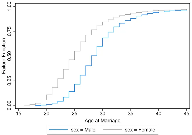
The vector Xi,t includes variables affecting the decision to marry. These may be partitioned into two main categories: (a) those which are – at least partially – decided by the agent, such as educational attainment, job participation, religious attendance, and (b) those which are not chosen, like family background. Whereas variables in category (b) are chosen in advance by other agents and then typi-cally time-invariant, variables in (a) are usually time-varying. A residual variable which varies across time but not depend on individual choices is the introduc-tion of divorce law. In what follows it is assumed that women and men show systematically different search behavior, because fertility periods differ for sexes (Siow, 1998) and women are more biologically constrained than men (Landsburg, 2000); also, the graphical assessment of hazard ratios in figs. (5) and (6) dis-play marked differences between sexes, with women marrying at an earlier age than men. Given these considerations, regressions were estimated separately for women and men, in order to clearly evaluate the interaction of different covari-ates with gender.

Divorce Law

Potentially, a change in divorce legislation can impact on the age at marriage or, equivalently, the probability of transition from singlehood to marriage, both by directly changing the option value of waiting for a better marriage opportunity and indirectly changing the choice variables that influence age at marriage, like education or job status. When examining the role played by legal innovation in directly modifying the age at marriage, the interest is in the following difference:

∆ _=Eh_hAD_{i,t −h}BD_i,t i_{= E}h_hiAD_{,t |After Divorce}i_−Eh_hBD_{i,t |Before Divorce}i ₍₈₎

4. DESCRIPTION OFVARIABLES

The dummy variable then partitions individuals into three samples: (a) those who got married before the reform, (b) those who entered the marriage market before the reform and experienced the change during marital search, and (c) those who entered the marriage market after the reform was passed. This partition pro-vides an opportunity to use the Before-After (BA) estimator (Heckman, LaLonde, and Smith, 1999), assuming that agents from sample (a) and (c) are intrinsically identical with respect to their preferences and constraints, once we control for observable covariates inX_i,t. Consequently, the remaining difference in the age at marriage is attributable to the divorce law and to the interaction of the dummy with other covariates. To estimate such a model, Lee (2005, pp. 30-32) proposes the following linear specification:

log(h_i,t) =X_i′_,tβ+d_i,tX′_i,tζ+d_i,tχ+υi,t (9) whereβis the coefficient vector for explaining variables,ζis the coefficient vector for the explaining variables interacting with the dummy variable of the divorce law, χ is the coefficient for the same dummy variable, and υ is an error term whose structure also depends on the dummy variable. The value of χ captures any structural break occurring after the divorce law comes into force, while a comparison between βand ζ reveals whether the explaining variables changed their impact after the divorce law. Since the theory of marital search provides no straightforward hint on error specification, the issue is solved empirically in the estimation section. To account for any time trend occurring in the period under study which may confound the effect of the divorce law, the year of observation is inserted as a control in itself and also multiplied by the dummy.

Education

In marriage markets, like in other markets, rational agents tend to differentiate their own offer. In order to obtain extra benefits from the matching mechanism, people tend to escape the sluggishness of uniformity and signal themselves as ex-traordinary individuals. On the one hand, some signals can be deceitful: Match-ing theory has long demonstrated (Roth, 1984; Bergstrom and MannMatch-ing, 1982) that in every matching game agents tend to exaggerate their characteristics to climb the ladder of matching quality. On the other hand, some assets reveal real qualities that do make a big difference, and education is one of them. However, since education cannot be easily combined with marital life and child rearing, more educated individuals are expected to delay marriage until the process of acquiring an education is completed. When traditional gender roles prevail, then education should delay marriage more for women than for men. Higher levels of education may lead to a more productive search which would have an am-biguous effect on the duration of the search since direct search costs would be lowered, but the number of searches possible per unit time would be increased (Keeley, 1977). Nonetheless, more educated individuals may become more picky and selective: even in this case, the net impact of education is controversial and needs to be estimated.

4. DESCRIPTION OFVARIABLES

so it is a source of high and spurious correlation with the dummy for divorce law. To deal with this difficulty, the following strategy was used: first the aver-age level of education is estimated, with this averaver-age taken across sex, aver-age, and geographical location (North or South). Then this value is used to calculate the percent difference between the actual individual level of completed education in years and the appropriate average in the following way:

Differential Education= ei,t(h,η,σ)−e¯t(h,η,σ)

¯

et(h,η,σ)

where hstands for age,η stands for geographical location, andσ stands for sex. The termdifferential educationemphasizes only a measure of difference and not the whole stock of human capital itself. We used this variable instead of completed education in the regressions in order to dispel the pure effect of education net of any temporal exogenous increase in the same variable.

Do rational agents adjust their educational choices when divorce becomes an option? When married couples split, a higher level of education may help both partners find a better job and recover quicker from the financial losses from di-vorce. This hypothesis should prove correct especially for women, since they can compensate a weaker job status with stronger education to a greater extent than men. Whether differential education also impacts on age at marriage after the reform is an interesting point. Divorce law could make marriage markets more competitive since rents for bilateral monopoly are lowered by the exit option. The increased level of competition may drive agents to invest more in education to catch up with the best competitors. However, this results in an increase in the av-erage level of education, and agents with education above avav-erage become fewer. Across time, the distribution of education becomes more concentrated around the mean. Then, if preferences remain constant, the premium for differential educa-tion should become greater.

Occupational Status

fol-4. DESCRIPTION OFVARIABLES

lowing way: 0 for unemployed, 1 for occasional job, 2 for seasonal job, and 3 for stable job.

Interaction of divorce with job status also raises issues which parallel those raised by education. Though, since job status is directly related to income pro-duction, after divorce reform, its role in determining age at marriage could also be strengthened. A better job position creates incentives to matching for men since a stable job becomes more valuable when marriage duration becomes uncertain. Given that a stable job also functions as an insurance for the hard times which can follow from divorce (Lundberg and Pollak, 2003), women’s age at marriage should decrease as women participate more in the job market and obtain stable status.

Religious Attendance

Along with its economic, financial, and social facets, marriage also has strong religious importance. Almost any religion entails some form of celebration for marriage which attaches additional commitment to marital promises. For reli-gious people, this results in higher levels of marriage-specific investments and additional difficulties related to divorce. The current literature on marriage be-havior of Catholics in the US (Lehrer and Chiswick, 1993; Chiswick and Lehrer, 1990) suggests that these people tend to marry later, with a larger fraction than average remaining permanently single. Most probably, this depends on the per-ceived level of irreversibility of marriage, enforced by religious stigma. Since the mere declaration of Catholic identity could be misleading in a country like Italy where Catholicism is widely predominant, the variable used to control for reli-gious activity is yearly participation in relireli-gious ceremonies. This variable has seven time-invariant modalities, ranging from 0 (no participation in a year) to 7 (more than once a week). The variable also interacts the dummy for the introduc-tion of divorce to test how catholics reacted to this crucial innovaintroduc-tion in naintroduc-tional legislation. It must be borne in mind that Catholic Church does not forbid di-vorce per se, but only remarriage for didi-vorcees: those who remarry against the religious norm are not allowed to access the sacraments.

Family Background

at-5. ECONOMETRICRESULTS

titudes toward marriage. Regarding family size, it is likely that in large families parents usually cannot trade wealth against a longer stay in the house for their offspring, so its expected impact on the likelihood of marriage should be positive. The problem with including the previous four variables in equation (9) is the high level of collinearity they show. To prevent instability in the estimates, a standard Principal-Component analysis was used to compact the overall variability and results are displayed in tab. (4). The resulting first factor, which summarizes the effect of family background, was included in the model to be estimated.

5

Econometric Results

5.1

Sample and Estimation Procedure

The data used are taken from the Longitudinal Survey of Italian Families (ILFI) which is a retrospective survey recording information on current and past events of individual and family life.4 The first survey was held in 1997 and subse-quent ones were held every two year. The dataset contains a complete account of episodes of lives of individuals, ranging from education to marriage, and from geographical mobility to labor experience; with this episode structure, it is possi-ble to obtain an exact snapshot of the situation of an individual in a given moment and study it using event-history methodology.

To take into account systematic differences between sexes and in order to em-phasize them clearly, each regression was run separately for women and men. Three types of observations were excluded from the sample: (1) all subjects who married prior to 1950, since marital behavior during war time can be erratic due to exceptional circumstances impacting matching possibilities, education, and work; (2) observations prior to the age of 18, because marriage for individuals who are under age is subject to particular legal restrictions; (3) observations for people who do not marry before the 49th year of their life: this exclusion is due to the biological constraint on fertility, since late marriages presumably follow from alternative lifestyles which do not include children rearing. As a result of this se-lection, in all, the complete sample models contains 29,888 observations covering 2,664 men plus 26,046 observations covering 3,150 women. The mean number of observations per man is 11.2, while per woman is 8.3. The first two waves of the sample were included: this results in a pool of people being married not before 1950 and not later than 1999. Since in 1999 some agents are not yet married, an appropriate procedure was use to account for censoring.

Estimation of determinants of age at marriage requires setting up a statistical model specifying a functional form for eq. (9). Since many possible distributional specifications are available and the economic theory of marriage does not provide any clear-cut hint about them, we chose to adopt the function which best fits the sample. At first the unconditional hazard rate was plotted for men and women and reported in fig. 5 (the corresponding survivor functions are plotted in fig. 6). These figures show strong concavity in hazard rates: even though this is not unambiguous evidence of time-dependency of the hazard rate, it is likely that

5. ECONOMETRICRESULTS

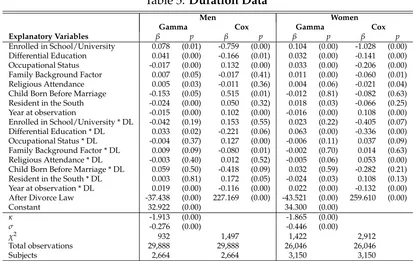
the largest fraction of marriages does happen during a well-defined time interval which roughly corresponds to the fertile section of adult life, and this holds true especially for women. A natural implication is that the hazard rate cannot be as-sumed to be constant over time, so that the exponential specification must be put aside. Next, we estimated the gender-based models over several competing dis-tributional assumptions. Results are reported in tab. (3). Relying on the Akaike Information Criterion (AIC) and Bayesian Information Criterion (BIC) (Ludden, Beal, and Sheiner, 1994; Koehler and Murphree, 1988), we find that the Gamma distribution fits the data best. The correspondingχ2values provide support for the Weibull distribution for women, but the difference with Gamma distribution is very limited. Thus, the choice for the parametrization to adopt is the Gamma function: estimation results for this specification are displayed in the first and third column of tab. (5).

One problem with parametric estimation is that a substantial interpretation can rarely be given to the parameters which are intrinsic to the distribution func-tion. Thus, an alternative way to frame the problem is to consider the baseline hazard as a nuisance and estimate it through a semi-parametric approach which does not rely on any distributional assumption. In our context, this procedure was performed using the Cox estimator and results are displayed in the second and fourth column of tab. (5).

Both for parametric and semi-parametric specifications, the standard errors were estimated using a bootstrap technique with 50 replications stratified over individuals. As regards the interpretation of the parameter sign, the two models are estimated using different metrics. The Gamma model employs the Acceler-ated Failure-Time (AFT) metric, while the Cox model employs the Log Relative-Hazard (LRH) metric. For example, a positive estimated coefficient in the AFT metric indicates longer durations for higher values of the covariate, while in the LRH metric a positive coefficients indicates higher probability of a transition of state for higher values of the covariate, which results in shorter durations. Ba-sically, when contrasting the two models, the statistically significant coefficients display opposite signs across the two models. With regard to interpretation of estimated parameters in the Cox model, it is worth recalling that the baseline hazard ψ(t) in eq. (7) is not parametrically estimated: hence, the only possible interpretations about the hazard rate can be made for changes in independent variables (Singer and Willett, 2003). A percentage variation in the hazard rate in response to a variation in the exogenous variable Xj from x0 tox1 can be

calcu-lated as follows _"

eβj(Xj=x1)_−eβj(Xj=x0)

eβj(Xj=x0)

#

·100. (10)

which in the case of a dummy variable reduces to[eβj_−1]·100.

5.2

Comments

introduc-5. ECONOMETRICRESULTS

tion of divorce law by shortening their search spells. Compared to the no-divorce scenario and other things being equal, marriage has become a riskier business both for men and women. However, in our sample people seem to respond to this change in the rules of the game by increasing their propensity to marry, which is puzzling since an increase in risk should produce a decrease in the demand for marriage. To solve this riddle, it is worth going back to the basic mechanics of marriage. As was noted in the theoretical section, marriage is a multiperiod contract, and a legal innovation introducing the possibility of breaking the con-tract impacts both on married couplesandindividual agents who are considering whether to marry. Following this legal change, married agents register a decrease in their reservation utility: the marriages which dissolve are those in which at least one partner prefers divorce to staying with the current partner. This ex-plains why during the years immediately following the introduction of divorce the number of divorces rocketed, as it is clear from fig.3. This was a temporary ef-fect due to the adjustment of the previous stock of marginal couples. Most likely, this legal innovation also changed the equilibrium within inframarginal couples, i.e. those who adjust to the new legislation but decide not to break; however, we do not investigate the issue in this article, since our focus is on single individuals who are considering whether to marry.

The impact of regime change on prospective marriages is twofold: on the one hand, since marriage implies idiosyncratic investments, the possibility of uni-lateral divorce makes the contract riskier. Consequently, risk-adverse partners should become more cautious when considering the option of marriage. Some of these people may decide not to marry at all, while others may become more selective. As a result, the average length of search spell registers an increase. Moreover, should the marriage prove unsatisfactory, each partner is given by the law the possibility to break it – bearing a fraction of its cost – and possibly starting another marriage anew. In the search process, this innovation pushes individu-als to become less picky since divorce is a way out from a bad marriage: the outcome would be a decrease in the average length of search spell. Economic theory of marriage has no clear prediction on the net effect of these two contrast-ing forces. Our estimation results suggest that, on balance, what prevails between these two opposing forces is the increased utility deriving from the availability of the new exit option.

An alternative way to model this balance of forces, although it is not very com-mon in marriage economics literature, consists in framing the decision to marry in the context of modern investment theory.5 While traditional theory investigates the binary choice between investing and not investing, the most recent theory based on option value stresses the role played by irreversible actions and fixed costs. Since the first marriage entails a permanent change in personal status, peo-ple can choose rationallywhento exercise the option of marrying. A basic result of option value theory says that the more irreversible an investment, the longer will be the period spent waiting to use the related option. In our model, a

mar-5_{In fact, the best book to date on the subject (Dixit and Pindyck, 1994), calls for an extensive use}

5. ECONOMETRICRESULTS

riage which does not include the possibility of divorce is more irreversible than a marriage in which individuals can divorce unilaterally when individual utility falls below a given threshold. Hence, the change in divorce legislation promotes shorter search spells. Our evidence suggests that Italian couples respond to in-centives related to irreversibility and decreased waiting time. In terms of the tra-ditional theory of marriage, our data show individuals put a heavier weight on the possibility of escaping a bad marriage rather than on the security of a life-long marriage.

From estimation results it is evident that women reacted more than men to the change in legislation. A possible explanation for this result is that women on av-erage are more constrained than men in their search for matching partners, given that their biological clock related to fertility ticks faster than men’s. A lower level of irreversibility, from a woman’s standpoint, could be valued more positively than from a man’s perspective since it lowers the penalty related to a bad match. Consequently, women should discount less than men the possibility of marriage break-up and their search strategy is more affected by the exit option than men’s. To control for the confounding effect of the time trend on the dummy vari-able for divorce, year at observation was inserted to account for aggregate trend which reflects unobservable changes. The estimated values show decreasing age at marriage before 1971, with a strong structural break occurring at 1971, and then an almost flat tendency.

5. ECONOMETRICRESULTS

in the educational system, women become less prone to marry since this could lead to study interruption or canceling. This reflects that, after divorce, education becomes more valuable for women than for men.

Differential education also plays a role in determining age at marriage, but this is reflected in an increase in age at marriage. A man endowed with educa-tion which is 10% higher than the reference pool of marriageable men, faces a -80.9% decrease in his hazard rate, while women face -75.5% decrease. This sur-prisingly small gender difference is probably attributable to the effect that extra education plays in the marriage market for women. Most probably, these agents face larger difficulties compared to agents with negative differential education, since the former tend to match with similar types which are quite rare in the marriage market, so their search becomes longer. After the divorce reform took place, the negative effect of differential education became stronger both for men and women: the same increase of 10% in differential education for women results in a chance in the hazard rate of -99.2%. Since differential education is mainly a positional good, this variation across time may reflect the higher level of average education among women and a decreased dispersion around the mean.

Job status displays strong asymmetric effects on sexes. The effect of changing job status from unemployment to a stable job increases men’s age at marriage by 48.4%, while for women the change is -46.0%: the two values are virtually the opposite of one another. An enhancement in job status has a positive impact on the probability of marriage for men and tends to decrease their search spell; on the contrary, a positive variation in the same variable makes marriage less likely for women and delays it. Men with better positions in the job market can afford marriage more easily, since they are able to support a family on a stable basis, and prospective partners of the opposite sex attach value to this asset. These results provide evidence that unemployment or job instability make men less likely to marry. On the contrary, women who are stronger in the job market probably face greater difficulties in marrying since home production and child rearing can be matched with working outside the house only at a substantial cost. Thus, we have a substitution effect on marriage probability: a more stable job implies lower gains from trade and a decreased propensity to marry for women. Furthermore, when traditional gender roles prevail, the same men have higher gains from trade in marriage, so they are likely to marry for they lose much from being single. This finding corroborates Becker’s result that high income should create incentives for men not to marry late (Becker, 1991). From estimation results, the change in legislation impacted the role played by job position in determining the hazard rate. The transition from unemployment to a stable job now results in a 117.2% increase for men, while it results in a -39.7% decrease for women. This shows a 11.8% decrease in the penalty attached to stable job. As expected, this last result confirms that after divorce reform, the marriage market for women adjusted to the new strategic role of job status.

6. SUMMARY ANDCONCLUDINGREMARKS

is consistent with previous literature showing that high levels of service atten-dance and religious involvement for Catholics tend to delay marriage because of the high perceived irreversibility. More interestingly, the impact of religious attendance when divorce is allowed by national law (but not by Catholic law) is reversed: it becomes positive, with a value around 21.2%. This reversed trend may result from the new emphasis given by the Catholic Church to traditional family after 1971, combined with increased strong prohibitions of pre-marital sex and abortions, which drove young Catholic women towards earlier marriages. Family Background and Other Controls. According to the estimation results, the role played by family background on the search spell is of mild importance. For men it is significant only after 1971, while for women the value remains the same across the whole sample and the magnitudes of the effects are basically constant across genders. Since parents’ education is positively related to the factor, and given that the estimated parameter in the Cox model is negative, an increase in parental education decreases the likelihood of marriage. In general, more edu-cated parents place a high value on the education of their children and tend to create wealthier families and emotionally comfortable environments, thereby in-creasing the reservation value of leaving the parental nest. In addition, the larger the family, the more traditional the gender expectations will be for the offspring: young women are required to help their parents and siblings, while men are re-quired to find a job and leave the parents’ house. Furthermore, all other variables held constant, larger families usually display lower levels of average consump-tion, a factor which is likely to work against long spells of singlehood.

Another control was geographical location, since systematic differences in the economic and social performance of southern and northern Italian regions are commonly observed (Barbagli, Castiglioni, and Dalla Zuanna, 2003; Schizzerotto, 2002; Barbagli and Saraceno, 1997). The dummy control variable for geographical location interacted with the divorce law provides weak evidence that residence in the South tends to decrease women’s search spell by a value close to 4.2%, while for men the percentage change is around 24.9%, although the p-values suggest significance just for a limited fraction of the sample.

The last control introduced in the regression models is a dummy variable for a child born before marriage. The main effect is on men, both before and after the divorce law. Before the divorce law, a child born increases the hazard ratio by 67.4%; after the divorce law, this value decreases to 10.2%. From our sample, women seem to be affected by out-of-wedlock births in a very limited way.

Year at observation was inserted to take account of aggregate trends which reflect unobservable changes. The estimated values show decreasing age at mar-riage before 1971, with a strong structural break occurring in 1971, and then an almost flat tendency.

6

Summary and Concluding Remarks

6. SUMMARY ANDCONCLUDINGREMARKS

provide an interesting fount of natural experiment.

In the theoretical section, the underlying microeconomic model is based on the assumption that agents sample sequentially from a given distribution of available mates and choose optimally whether to accept a marriage offer, given their en-dowment of specific personal traits. Some of these traits are exogenously given, such as the family background or current conditions in the marriage market, while others are a matter of choice, such as investment in education or the level of involvement in the labor market. When divorce is not permitted by law, the decision to marry is irreversible, while the introduction of divorce introduces the possibility of serial marriages. This innovation creates incentives to change search behavior since marital investment becomes riskier, but divorce is also an exit op-tion.

In the empirical section, we tested the effect of the new divorce legislation on the probability of marriage. The dummy variable for the introduction of divorce was inserted into the complete sample, whereas the same dummy was interacted with other variables which are a matter of choice. Other variables at the personal and at the environmental levels were included to control for confounding effects. Results show that the very introduction of divorce reduced the average search spell, since availability of a new exit option makes the decision to marry less irre-versible than it was in the past. This interpretation is consistent with the option value theory of investment.

6. SUMMARY ANDCONCLUDINGREMARKS

Results

Table 1: Summary Statistics

Variable Mean (Std. Dev.) Min. Max. N

Enrolled in School/University 0.19 (0.39) 0 1 78259

Differential Education 0 (0.45) -1.52 2.55 78259

Occupational Status 1.75 (1.45) 0 3 78259

Family Background Factor -0.05 (1.36) -6.24 5.72 78259

Religious Attendance 3.45 (2.03) 1 7 78259

Child Born Before Marriage 0.01 (0.12) 0 1 78259

Resident in the South 0.4 (0.49) 0 1 78259

Year at observation 1970.99 (14.55) 1926 1999 78259

After Divorce Law 0.51 (0.5) 0 1 78259

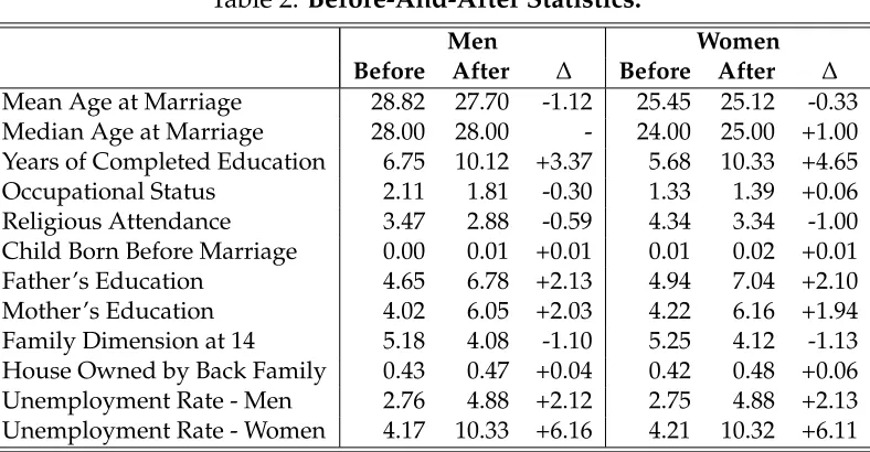
Table 2: Before-And-After Statistics.

Men Women

Before After ∆ Before After ∆

Mean Age at Marriage 28.82 27.70 -1.12 25.45 25.12 -0.33 Median Age at Marriage 28.00 28.00 - 24.00 25.00 +1.00 Years of Completed Education 6.75 10.12 +3.37 5.68 10.33 +4.65 Occupational Status 2.11 1.81 -0.30 1.33 1.39 +0.06 Religious Attendance 3.47 2.88 -0.59 4.34 3.34 -1.00 Child Born Before Marriage 0.00 0.01 +0.01 0.01 0.02 +0.01 Father’s Education 4.65 6.78 +2.13 4.94 7.04 +2.10 Mother’s Education 4.02 6.05 +2.03 4.22 6.16 +1.94 Family Dimension at 14 5.18 4.08 -1.10 5.25 4.12 -1.13 House Owned by Back Family 0.43 0.47 +0.04 0.42 0.48 +0.06 Unemployment Rate - Men 2.76 4.88 +2.12 2.75 4.88 +2.13 Unemployment Rate - Women 4.17 10.33 +6.16 4.21 10.32 +6.11

Table 3:Comparison between competing distributional specifications. Model LL(null) LL(model) df AIC BIC χ2

Men Weibull -27.02 436.70 13 -847.40 -733.60 603.05

Gamma 940.94 1,271.11 13 -2,516.21 -2,402.41 587.37 Log-Normal 740.84 1,098.06 12 -2,172.11 -2,067.07 601.75 Log-Logistic 847.58 1,232.27 12 -2,440.55 -2,335.50 628.03 Exponential -4,022.50 -1,723.33 11 3,468.65 3,564.94 3,675.97

Gompertz -650.58 -21.98 12 67.97 173.01 853.62

Women Weibull -645.28 185.66 12 -347.31 -245.11 865.90

6. SUMMARY ANDCONCLUDINGREMARKS

Table 4:Principal Component Analysis of Family Background

Comp1 Comp2 Comp3 Comp4 Comp5

Father’s Education 0.609 0.346 -0.067 0.102 -0.704

Mother’s Education 0.615 0.328 -0.061 0.074 0.710

House Owned by Back Family -0.049 0.271 0.961 0.002 -0.000

Family Dimension at 14 -0.407 0.514 -0.168 0.736 0.024

Only Child 0.288 -0.660 0.200 0.665 0.003

Table 5: Duration Data

Men Women

Gamma Cox Gamma Cox Explanatory Variables β p β p β p β p

Enrolled in School/University 0.078 (0.01) -0.759 (0.00) 0.104 (0.00) -1.028 (0.00)

Differential Education 0.041 (0.00) -0.166 (0.01) 0.032 (0.00) -0.141 (0.00)

Occupational Status -0.017 (0.00) 0.132 (0.00) 0.033 (0.00) -0.206 (0.00)

Family Background Factor 0.007 (0.05) -0.017 (0.41) 0.011 (0.00) -0.060 (0.01)

Religious Attendance 0.005 (0.03) -0.011 (0.36) 0.004 (0.06) -0.021 (0.04)

Child Born Before Marriage -0.153 (0.05) 0.515 (0.01) -0.012 (0.81) -0.082 (0.63)

Resident in the South -0.024 (0.00) 0.050 (0.32) 0.018 (0.03) -0.066 (0.25)

Year at observation -0.015 (0.00) 0.102 (0.00) -0.016 (0.00) 0.108 (0.00)

Enrolled in School/University * DL -0.042 (0.19) 0.153 (0.55) 0.023 (0.22) -0.405 (0.07)

Differential Education * DL 0.033 (0.02) -0.221 (0.06) 0.063 (0.00) -0.336 (0.00)

Occupational Status * DL -0.004 (0.37) 0.127 (0.00) -0.006 (0.11) 0.037 (0.09)

Family Background Factor * DL 0.009 (0.09) -0.080 (0.01) -0.002 (0.70) 0.014 (0.63)

Religious Attendance * DL -0.003 (0.40) 0.012 (0.52) -0.005 (0.06) 0.053 (0.00)

Child Born Before Marriage * DL 0.059 (0.50) -0.418 (0.09) 0.032 (0.59) -0.282 (0.21)

Resident in the South * DL 0.003 (0.81) 0.172 (0.05) -0.024 (0.03) 0.108 (0.13)

Year at observation * DL 0.019 (0.00) -0.116 (0.00) 0.022 (0.00) -0.132 (0.00)

After Divorce Law -37.438 (0.00) 227.169 (0.00) -43.521 (0.00) 259.610 (0.00)

Constant 32.922 (0.00) 34.300 (0.00)

κ -1.913 (0.00) -1.865 (0.00)

σ -0.276 (0.00) -0.446 (0.00)

χ2 _{932 1,497 1,422 2,912}

Total observations 29,888 29,888 26,046 26,046

6. REFERENCES

References

ALLEN, D. (1992): “Marriage and Divorce: Comment,” The American Economic

Review, 82(3), 679–685.

ALLEN, D., K. PENDAKUR, AND W. SUEN (2006): “No-Fault Divorce and the

Compression of Marriage Ages,”Economic Inquiry, 44(3), 547.

BARBAGLI, M., M. CASTIGLIONI, AND G. DALLA ZUANNA (2003): Fare famiglia in Italia: un secolo di cambiamenti. Il Mulino.

BARBAGLI, M.,ANDC. SARACENO(1997):Lo stato delle famiglie in Italia. Il Mulino.

BECKER, G. S. (1991):A Treatise on the Family (Enlarged Edition). Harvard Univer-sity Press, Cambridge and London.

BERGSTROM, T.,ANDR. MANNING(1982): “Can Courtship Be Cheatproof?,” also

available at: http://www.econ.ucsb.edu/~tedb/Family/courtship.pdf.

BERGSTROM, T., AND R. F. SCHOENI (1996): “Income Prospects and

Age-at-Marriage,”Journal of Population Economics, 9(2), 115–30.

BOUGHEAS, S.,ANDY. GEORGELLIS(1999): “The Effect of Divorce Costs on

Mar-riage Formation and Dissolution,”Journal of Population Economics, 12, 489–498. BRIEN, M., ANDL. LILLARD(1994): “Education, Marriage, and First Conception

in Malaysia,”The Journal of Human Resources, 29(4), 1167–1204.

BURDETT, K., AND M. G. COLES (1997): “Marriage and Class,” The Quarterly

Journal of Economics, 112(1), 141–168.

BURDETT, K., AND M. G. COLES (1999): “Long-Term Partnership Formation:

Marriage and Employment,” Economic Journal, 109(127), F307–34, available at http://ideas.repec.org/a/ecj/econjl/v109y1999i456pf307-34.html.

BURDETT, K.,ANDD. T. MORTENSEN(1978): “Labor Supply under Uncertainty,”

inResearch in Labor Economics, ed. by R. G. Ehrenberg, vol. 2, pp. 109–158. JAI Press, Greewich, Conn.

BURGESS, S., C. PROPPER, AND A. AASSVE(2003): “The Role of Income in

Mar-riage and Divorce Transitions Among Young Americans,”Journal of Population Economics, 16(3), 455–475.

CHIAPPORI, P., B. FORTIN, ANDG. LACROIX(2002): “Marriage Market, Divorce

Legislation, and Household Labor Supply,”Journal of Political Economy, 110(1), 37–72.

CHISWICK, C., AND E. LEHRER (1990): “On Marriage-specific Human Capital,”

Journal of Population Economics, 3(3), 193–213.

CORNELIUS, T. (2003): “A Search Model of Marriage and Divorce,” Review of

6. REFERENCES

DEVINE, T. J., AND N. M. KIEFER (1991): Empirical Labor Economics – The Search

Approach. Oxford University Press, Oxford.

DIXIT, A.,AND R. PINDYCK (1994): Investment Under Uncertainty. Princeton Uni-versity Press Princeton, NJ.

FILOSO, V. (2005): “Why Love Matters - A Dynamic Model

of Marriage and Divorce,” Labor and Demography 0505003,

Economics Working Paper Archive EconWPA, available at

http://ideas.repec.org/p/wpa/wuwpla/0505003.html.

FRIEDBERG, L. (1998): “Did Unilateral Divorce Raise Divorce Rates? Evidence from Panel Data,”The American Economic Review, 88(3), 608–627.

GRAY, J. (1998): “Divorce-Law Changes, Household Bargaining, and Married

Women’s Labor Supply,”The American Economic Review, 88(3), 628–642.

GRUBER, J. (2004): “Is Making Divorce Easier Bad for Children? The Long-Run

Implications of Unilateral Divorce,”Journal of Labor Economics, 22(4), 799–833. HECKMAN, J., R. LALONDE, AND J. SMITH (1999): “The Economics and

Econo-metrics of Active Labor Market Programs,” inHandbook of Econometrics, ed. by Z. Griliches,andM. D. Intriligator, vol. 3, pp. 1865–2097. Amsterdam.

HECKMAN, J. J.,ANDT. E. MACURDY(1986): “Labor Econometrics,” inHandbook

of Econometrics, ed. by Z. Griliches,andM. D. Intriligator, vol. 3, chap. 32, pp. 1918–1977. Elsevier Science, Amsterdam.

KEELEY, M. C. (1977): “The Economics of Family Formation,” Economic Inquiry,

15, 238–250.

KOEHLER, A., AND E. MURPHREE (1988): “A Comparison of the Akaike and Schwarz Criteria for Selecting Model Order,”Applied Statistics, 37(2), 187–195. LANCASTER, T. (1990): The Econometric Analysis of Transition Data, Econometric

Society Monographs. Cambridge University Press, New York, NY.

LANDSBURG, S. E. (2000): “Why Men Pay To Stay Married. And Women Pay to

Get Divorced,”Slate.

LEE, M.-J. (2005): Micro-Econometrics for Policy, Program, and Treatment Effects.

Oxford University Press, New York.

LEHRER, E., AND C. CHISWICK (1993): “Religion as a Determinant of Marital Stability,”Demography, 30(3), 385–404.

LIPPMAN, S. A., AND J. J. MCCALL (1976): “The Economics of Job Search: A

Survey,”Economic Inquiry, 14(3), 347–68.

LJUNGQVIST, L., AND T. J. SARGENT (2000): Search, Matching, and

6. REFERENCES

LUDDEN, T., S. BEAL, AND L. SHEINER (1994): “Comparison of the Akaike

In-formation Criterion, the Schwarz criterion and the F test as guides to model selection,”Journal of Pharmacokinetics and Pharmacodynamics, 22(5), 431–445. LUNDBERG, S., AND R. POLLAK (2003): “Efficiency in Marriage,”Review of

Eco-nomics of the Household, 1(3), 153–167.

MATSUSHITA, K. (1989): “Economic Analysis of Age at First Marriage,”Journal of

Population Economics, 2, 103–119.

MICHAEL, R., AND N. TUMA (1985): “Entry Into Marriage and Parenthood by

Young Men and Women: The Influence of Family Background,” Demography, 22(4), 515–544.

MORTENSEN, D. T. (1986): “Job Search and Labor Market Analysis,” inHandbook

of Labor Economics, ed. by O. Ashenfelter, and R. Layard, vol. 2, chap. 15, pp. 849–919. Elsevier Science, Amsterdam.

PETERS, H. E. (1986): “Marriage and Divorce: Informational Constraints and

Private Contracting,”American Economic Review, 76(3), 437–54.

(1992): “Marriage and Divorce: Reply,”American Economic Review, 82(3), 686–693.

ROTH, A. E. (1984): “Misrepresentation and Stability in the Marriage Problem,”

Journal of Economic Theory, 34, 383–387.

SCHIZZEROTTO, A. (2002): Vite ineguali: disuguaglianze e corsi di vita nell’Italia

con-temporanea. Il mulino.

SINGER, J., AND J. WILLETT (2003): Applied Longitudinal Data Analysis: Modeling

Change and Event Occurrence. Oxford University Press.

SIOW, A. (1998): “Differential Fecundity, Markets, and Gender Roles,”Journal of

Political Economy, 106(2), 334–354.

STEVENSON, B. (2003): “The Impact of Divorce Laws on

Marriage-Specific Capital,” Working Paper 43, Harvard University, available at http://www.frbsf.org/publications/economics/papers/2006/wp06-43bk.pdf.

STEVENSON, B., ANDJ. WOLFERS (2006): “Bargaining in the Shadow of the Law:

Divorce Laws and Family Distress,”Quarterly Journal of Economics, 121(1), 267– 288.

STOKEY, N. L., R. E. LUCAS, AND E. C. PRESCOTT (1989): Recursive Methods in Economic Dynamics. Harvard University Press, Cambridge, MA.

STROBEL, F. (2003): “Marriage and the Value of Waiting,” Journal of Population Economics, 16(3), 423–430.

6. REFERENCES

WEISS, Y. (1997): “The Formation and Dissolution of Families: Why Marry? Who

Marries Whom? And What Happens Upon Divorce,” inHandbook of Population and Family Economics, ed. by M. R. Rosenzweig,and O. Stark, vol. 1a, chap. 3, pp. 81–123. Elsevier Science, Amsterdam.

WEISS, Y.,ANDR. J. WILLIS(1997): “Match Quality, New Information, and

Mar-ital Dissolution,”Journal of Labor Economics, 15(1), S293–S329.

WOLFERS, J. (2006): “Did Unilateral Divorce Laws Raise Divorce Rates? A

7. FIGURES

7

Figures

10

12

14

16

18

Nuptiality Rate

1950 1960 1970 1980 1990 2000

Year

Figure 1: Italian Nuptiality Rate (1950–2001).

24

26

28

30

32

Mean Age at Marriage

1950 1960 1970 1980 1990 2000

Year

Men Women

7. FIGURES

0

10

20

30

1950 1960 1970 1980 1990 2000

Year

Separations / Marriages Divorces / Marriages

Figure 3: Legal separations and divorces (1950–2001).

40

60

80

100

120

140

Graduated Women / Graduated Men

1950 1960 1970 1980 1990 2000

Year

7. FIGURES

0

.05

.1

.15

Smoothed Hazard Rate

15 20 25 30 35 40 45 50 55 60

Age at Marriage

sex = Male sex = Female

Smoothed hazard estimates, by sex

Figure 5: Smoothed hazard rates by sex.

0.00

0.25

0.50

0.75

1.00

Failure Function

15 20 25 30 35 40 45

Age at Marriage

sex = Male sex = Female

Kaplan−Meier failure estimates, by sex