Munich Personal RePEc Archive
An Extremely Low Interest Rate Policy
and the Shape of the Japanese Money
Demand Function: A Nonlinear
Cointegration Approach
Nakashima, Kiyotaka
Konan University
4 August 2008
An Extremely Low Interest Rate Policy and the
Shape of the Japanese Money Demand Function:
A Nonlinear Cointegration Approach
(Forthcoming in Macroeconomic Dynamics)
Kiyotaka Nakashima∗†
August 4, 2008
∗
Correspondence to: Kiyotaka Nakashima, Faculty of Economics, Konan University, 8-9-1,
Okamoto, Higashinada-ku, Kobe, Hyogo, Zip 658-8501, Japan, e-mail:
[email protected], phone: +81-078-435-2403, fax: +81-078-435-2543.
†
The author would like to thank Fumio Hayashi, Ryuzo Miyao, Yoji Morita, Makoto Saito,
and two anonymous referees for their helpful comments and encouragement. The author
Running Head: The Shape of the Japanese Money Demand Function
Name: Kiyotaka Nakashima
E-mail: [email protected]
Phone: +81-078-435-2403
Abstract
This paper explores the shape of the Japanese money demand function
in relation to the historical path of the Bank of Japan’s policy rate by
employing Saikkonen and Choi’s (2004) cointegrating smooth transition
model. The nonlinear model provides a unified econometric framework,
not only for pursuing the time profile of interest elasticity, but also to test
the linearity of the Japanese money demand function. The test results for
the linearity of the Japanese money demand function provide evidence of
nonlinearity with a semi-log model and linearity with a double-log model.
Using a nonlinear semi-log model, the analysis also finds that Japanese
money demand comprises three regimes and that the interest semi-elasticity
began to increase in the early 1990s when the Bank of Japan set the policy
rate below 3%.
JEL Classification Numbers: C22; E41; E58
1
Introduction
This paper empirically explores the shape of the Japanese M1 demand function
in relation to the historical path of the Bank of Japan’s (BOJ) policy rate using
the cointegrating smooth transition model in Saikkonen and Choi (2004).
From September 1995 onwards, the BOJ developed a unique low interest rate
policy (see Figure 1). While the BOJ initially guided overnight call rates below
0.5%, in February 1999 it implemented the so-called zero interest rate policy,
whereby the targeted overnight call rate was set at almost 0%. Accordingly,
the relative amount of money in circulation, as represented by M1 relative to
nominal GDP (the Marshallian k), rapidly increased towards 40% and higher
from the mid-1990s, even though it had been hitherto stable between 25% and
30%. In March 2001, the BOJ adopted a new policy framework by expanding
high-powered money. Although the quantity easing policy was lifted in March
2006, the targeted rate has since remained well below 0.5%.
The introduction of the low interest rate policy of the mid-1990s prompted
studies that focused on the shape of the Japanese money demand function from
the perspective of whether the Japanese economy had fallen into a liquidity
trap. Investigating the shape of the Japanese money demand function, given
the drastic increase in the Marshallian k under the small decrease in the call
rate since 1995, can be classified into the following aspects.
The first aspect is involved with the issue of whether Japanese money
(Miyao, 2004; Fujiki and Watanabe, 2004; Nakashima and Saito, 2006). Using
cointegrating structural break models constructed by Hansen (1992) and Kuo
(1998), these studies found that the absolute value of interest semi-elasticity
substantially increased in 1995, whereas that of the interest elasticity was stable
over time. 1 They confirmed that the estimates of interest elasticity ranged
from −0.11 to −0.15 for the full-sample periods under consideration and that
the estimates of interest semi-elasticity were −0.03 to −0.05 for sample periods
prior to 1995, whereas they were−0.4 to−0.6 for sample periods after 1995.
The second aspect is to investigate whether the Japanese money market has
a long-run equilibrium relationship. Previous studies, such as Miyao (2004) and
Fujiki and Watanabe (2004), have provided significant evidence of cointegration
in a double-log money demand model, but mixed evidence in a semi-log money
demand model. 2
The third aspect involves exploring a functional form to capture stable
Japanese money demand in terms of goodness-of-fit. Bae, Kakkar, and Ogaki
(2006) found that a double-log model outperformed a semi-log model in terms
of out-of-sample prediction performance. 3
The critical feature of previous studies on Japanese money demand is the
assumption of linearity for both the semi-log and double-log money demand
models. In the linear context, the test results for structural breaks show that
a double-log model can capture Japanese money demand over time without
could not without considering the change of interest semi-elasticity in 1995.
Further, the cointegration and goodness-of-fit test results commend use of the
double-log model, not the semi-log model.
One objective of this paper is to reassess the performance of the semi-log and
double-log money demand models. In particular, we evaluate the estimation and
test results of previous work by considering the possibility of nonlinearity in both
models. Both the semi-log and double-log models have their own theoretical
backgrounds and policy implications. 4 Indeed, as pointed out by Lucas (2000),
each model could derive a different policy implication if the level of nominal
interest rates was drastically lower than rates thus far, similarly to the Japanese
economy of the mid-1990s. 5 Hence, judging the advantage of one model over
the other requires careful examination.
There is another motivation that is common with existing empirical studies
on Japanese money demand: we investigate the shape of the Japanese money
demand function. However, the approach adopted in this paper differs from
previous studies in that we consider the time-varying interest elasticity (or
semi-elasticity) as a function of the BOJ’s policy rate. To fulfill our objectives, we
employ the cointegrating smooth transition model in Saikkonen and Choi (2004).
Analyzing the history of interest elasticity (or semi-elasticity) in relation to
a policy rate requires a state-dependent cointegrating model, that is, a model in
which the coefficient parameter in question depends on the state of an
accompanied by their cointegration test (Choi and Saikkonen, 2005) and
linear-ity test (Choi and Saikkonen, 2004), provides a unified econometric framework,
not only to estimate the time-varying interest rate elasticity, but also to evaluate
existing empirical studies on Japanese money demand under the extremely low
interest rate regime.
Careful examination of the shape of money demand requires a transition
value of a nominal interest rate, around which the interest elasticity is
fluctu-ating. Another advantage of Saikkonen and Choi’s (2004) model is that it can
identify the transition value. Other nonlinear cointegrating models (e.g., Park
and Phillips, 1999, 2001; Chang, Park, and Phillips, 2001; Bae and de Jong,
2007) and the cointegrating structural break models cannot identify this
tran-sition value. This paper attempts to uncover the shape of the Japanese money
demand function by identifying the historical path of interest elasticity and the
transition value of the BOJ’s policy rate.
In this paper, the nonlinearity of the smooth transition model concerns
mod-eling the long-run equilibrium of Japanese money demand, not the short-run
er-ror correction process to the equilibrium. Within a linear cointegration context,
the theory of nonlinear error correction models including smooth transition error
correction models has been developed by Saikkonen (2005, 2008) as an
exten-sion of Granger’s representation theorem, which provides a link between linear
cointegration and linear error correction models. 6 Within a nonlinear
dependent, however, an extension of Granger’s representation theorem has not
been developed. Consequently, this paper focuses on characterizing the long-run
Japanese money demand by using the cointegrating smooth transition model in
Saikkonen and Choi (2004). 7
The paper is organized as follows. Section 2 introduces a cointegrating
smooth transition model for Japanese money demand and discusses the
esti-mation and test results. In this section, we reassess the performance of the
semi-log and double-log models in terms of goodness-of-fit. Section 3 considers
the shape of the Japanese money demand function based on estimates obtained
in Section 2. Finally, Section 4 summarizes our empirical findings and discusses
some issues for future research. The Appendix details the simulation methods
and results.
2
Estimation and Test
In this section, we introduce a nonlinear model of Japanese money demand
based on Saikkonen and Choi’s (2004) cointegrating smooth transition model.
In general, a smooth transition model, in identifying the transition value of an
explanatory variable, deals with the dependence of a coefficient parameter on
the state of the explanatory variable. 8
In particular, Saikkonen and Choi’s (2004) nonlinear cointegrating model has
an econometric framework to conduct tests for the null hypotheses of
money demand, with few reservations, assumed linearity for both the semi-log
and double-log money demand models. However, if their assumption of
linear-ity were invalid, their test results for cointegration and goodness-of-fit would be
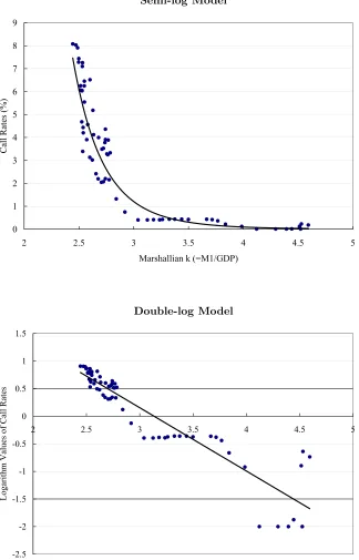
forced into a reexamination in a nonlinear context. Indeed, and according to
Figure 2, a double-log model appears to be linear, whereas a semi-log model
appears to be strongly nonlinear.
In this section, we undertake the following empirical steps. First, we find
a cointegrating relationship with possible nonlinearity for each of the semi-log
and double-log models. Next, we conduct the linearity test for the two models.
If we find nonlinearity, we reassess the performance of the two models in terms
of goodness-of-fit through modeling nonlinearity. Lastly, given the presence of
nonlinearity, we estimate a nonlinear money demand model.
2.1 Nonlinear Model of Money Demand
We assume that the Japanese money demand function can be described by the
following smooth transition model:
kt= constant +αit+βit
1− 1
1 + exp (−γ(it−i∗))
+ǫt, (1)
wherektindicates the logarithm of the Marshallian k, that is, the ratio of nominal
money stock to nominal GDP. Therefore, we adopt the velocity-based
specifi-cation for the Japanese money demand function. 9 In the semi-log model, it
gistic function 1+exp (−γ1(it−i∗)) makes the coefficient ofitvary smoothly between
α and α+β. When the value ofit sufficiently exceeds the transition value i∗,
the coefficient forit takes a value close toα. When the value ofit decreases and
is far below the transition value, the coefficient for it changes and approaches
α+β. Furthermore, β = 0 reduces the nonlinear money demand model to a
conventional linear model.
We build the set of quarterly data as follows. As nominal monetary
aggre-gates we choose M1, compiled and seasonally adjusted by the BOJ, because M1
reflects to a greater extent the transaction demand for money and hence is
fre-quently employed in empirical studies of the Japanese money demand function.
Nominal GDP, as constructed by the Statistics Bureau, is used for nominal
ag-gregate output. The overnight call rate, as reported by the BOJ, is used not
only as the BOJ’s policy rate but also as the opportunity cost of holding money.
10 Given the historical path of the call rate, regarded as the BOJ’s policy rate,
we should carefully choose the sample periods for inclusion. One strategy is to
include sample periods prior to February 1999 when the BOJ began the zero
interest rate policy. The inaction of the call rate at their lower bound (0%) for
long-term periods (from 1999 to at least 2006) would cause serious econometric
problems with our nonstationary and cointegration analysis. Existing nonlinear
cointegration techniques including Choi and Saikkonen (2004) cannot deal with
the prolonged inaction of the short-term nominal interest rates above the zero
Another strategy is to include sample periods prior to March 2001, when
the BOJ initiated the quantity easing policy. The departure from the policy
regime of interest rate targeting prohibits us from assuming that the call rate
reflects the BOJ’s policy decisions. 11 In addition, for the sample period prior
to August 2001, the short-term nominal interest rates stayed at low levels, but
barely moved above zero rates over time. For the following, we employ a strategy
of using sample periods up to the first quarters of 1999 and 2001; thereafter, we
check the robustness of the estimation and test results.
We conducted unit root tests for each of the variables: the log of the
Mar-shallian k, the level of the call rate, and the log of the call rate. We performed
augmented Dickey–Fuller (1979) and Phillips–Perron (1988) tests using data
from 1980 to 1999 or 2001. These test results confirm that each variable has a
unit root.
2.2 Nonlinear Estimation Method and Cointegration Test
In this section, we find the presence of a cointegrating relationship with possible
nonlinearity for the semi-log and double-log models using Choi and Saikkonen’s
(2005) test.
Choi and Saikkonen’s (2005) cointegration test is based on the following
two-step estimation procedure in Saikkonen and Choi (2004), which gives a consistent
and efficient estimator of the five parameters (constant, α, β, γ, i∗). For
function 1+exp (−γ1(it−i∗)) asg(it;τ), whereτ = (γ, i∗)′.
The first step of the estimation involves obtaining a conventional nonlinear
least squares (NLLS) estimatorθT with respect to θ. Although the NLLS
esti-mator is consistent, it is not efficient because of the regressor-error dependence.
12 Thereafter, to control the regressor-error dependence and thus obtain an
ef-ficient estimator, Saikkonen and Choi (2004) suggest considering the following
auxiliary regression model by adding the short-run dynamics ofit:
kt= constant +αit+βit(1−g(it;τ)) + K
s=−K
πs∆it−s+µt.
Plugging in the NLLS estimator θT, the second step of the estimation involves
obtaining the following efficient estimator forθ and π= (π−K. . . πK)′:
θ1T
π1 T = θT 0 + T−K
t=K+1 ztz′t
−1
T−K
t=K+1 zt′˜ǫt
,
wherezt=
βTit−∂g(it;τT) ∂τ
′
, 1, it, it(1−g(it;τT)), ∆it−K, . . . ,∆it+K
′
and
˜
ǫt indicate the fitted residuals in equation (1) using the NLLS estimates θT.
Saikkonen and Choi (2004) term the efficient estimator θ1
T as the “one-step
Gauss–Newton estimator.” They also propose plugging in the one-step Gauss–
Newton estimator instead of the NLLS estimator. They term the estimator
obtained in this manner the “two-step Gauss–Newton estimator.”
To test for cointegration in a nonlinear context, Choi and Saikkonen (2005)
propose a test for the null hypothesis of cointegration with possible nonlinearity
test for the null of stationarity. They develop the cointegration test for the case
of the NLLS estimatorθT and the one-step Gauss–Newton estimatorθ1T.
Accord-ing to Choi and Saikkonen (2005), the KPSS test usAccord-ing full-sample regression
residuals has limiting distributions that depend on unknown nuisance parameters
caused by the parameters of the models and regressor-error dependence.
Accord-ingly, they propose the use of subsamples of the regression residuals with block
size b and select the one that yields the maximum statistical values obtained
by applying the KPSS test to each of the subsamples. The subresidual-based
tests are not affected by the unidentified nuisance parameters. The selection
of the block size b can be done by using the minimum volatility rule proposed
by Romano and Wolf (2001). The rule comprises choosingb from b=bsmall to
b = bbig to minimize the standard deviations of 2m+ 1 statistical values that
are calculated in the neighborhood ofb, where m denotes an integer such that
m ≥ 1. 13 Choi and Saikkonen (2005) demonstrate that the calculated test
statistics asymptotically converge to1
0 w2(r)dr, wherew(r) denotes a standard Brownian motion. 14
Table 1 reports the test statistics and p-values of Choi and Saikkonen’s test
using the minimum volatility rule together with the selected block sizes. CθT
and Cθ1
T denote cointegration tests based on the NLLS estimation and the
one-step Gauss–Newton estimation with K = 1,2,4, respectively. To calculate the
test statistics, we setbmin = 10 and bbig =T −4, and choose m= 2 as in Choi
two cases, that is, sample periods from 1980/I and sample periods from 1985/I
to check the robustness of the tests. The null hypothesis is cointegration with
possible nonlinearity; we would be unable to reject cointegration for high
p-values. The null hypothesis cannot be rejected at 5% or lower in the various
periods, and consequently, we have strong evidence in favor of cointegration for
both the semi-log and double-log models in equation (1).
Our test results for cointegration with possible nonlinearity are noteworthy
because some empirical studies on Japanese M1 demand have pointed out the
possibility of no-cointegration with the semi-log model in the linear context of
β = 0 for equation (1). In contrast to previous work, our test results provide
strong evidence that not only the double-log model but also the semi-log model
has a cointegrating relationship with possible nonlinearity.
The small sample properties of the nonlinear cointegration test are reported
in the Appendix. As detailed, our test results are not subject to serious small
sample problems.
2.3 Linearity Test
As discussed earlier, previous research on the Japanese money demand function
assumed linearity for both the semi-log and double-log money demand models.
In this subsection, we evaluate the assumption of linearity.
We are interested in testing the null hypothesis that the money demand
hypothesis of interest is β = 0, while the alternative is β = 0. However,
con-ventional hypothesis testing is difficult because the nuisance parameters γ and
i∗ are not identified under the null hypothesis. Hence, for the linearity test of
β = 0, we employ the first-order (T1) and the third-order (T2) tests suggested
by Choi and Saikkonen (2004).
To calculate theT1 test in the semi-log model of equation (1), the log of the
Marshallian k is regressed on the call rate, the lead and lags of the differenced
call rate, and the call rate to the second power using OLS techniques. For the
T2 test in the semi-log model, the call rate to the third power is additionally
used as a regressor in the specification used for theT1 test. As demonstrated by
Choi and Saikkonen (2004), the linearity tests of β = 0 in T1 and T2 reduce to
testing the significance of a parameter estimate for the second power of the call
rate and the significance of parameter estimates for the second and third powers
of the call rate, respectively. To calculate the two tests in the double-log model
of equation (1), the logarithm value of the call rate should be used. The limiting
null distributions of theT1 and theT2 test statistics are chi-square distributions
with one and two degrees of freedom, respectively.
Table 2 illustrates the results of the linearity tests in the semi-log and
double-log models. First, for the semi-double-log model, the null of linearity is rejected at a
significance level of 5% in all cases of leads-lags and sample periods. For the
double-log model, on the other hand, the null is not rejected in almost all cases.
consideration of nonlinearity to capture Japanese M1 demand over time, whereas
the double-log model does not.
Our test results for linearity establish the validity of assuming a linear
spec-ification, at least for the double-log model, but not for the semi-log model. 15
The Appendix reports the small sample properties of theT1 and T2 tests for
linearity. As demonstrated, the two tests are not subject to serious small sample
problems.
2.4 Performance Comparison
In this subsection, we conduct a performance comparison of the four models in
equation (1)—the linear semi-log model, the linear double-log model, the
nonlin-ear semi-log model, and the nonlinnonlin-ear double-log model—in terms of
goodness-of-fit.
Table 3 reports the sum of squared error (SSE) for the four models. The
linear semi-log and double-log models are estimated with the fully modified OLS
in Phillips and Hansen (1990). The SSE for the nonlinear semi-log and
double-log models are based on estimates obtained using the two-step Gauss–Newton
estimator withK = 1. The following results do not depend on the structure of
the leads and lags. The SSE is calculated using the in-sample and out-of-sample
prediction errors.
The linear semi-log and nonlinear double-log models are clearly inferior to
perfor-mance. In particular, the result for the linear semi-log model is compatible with
that of Bae, Kakkar, and Ogaki (2006) who have shown that the linear
semi-log model is inferior to the linear double-semi-log model in terms of out-of-sample
prediction performance. On the other hand, the overall performance of the
non-linear semi-log model appears to exceed that of the non-linear double-log model. For
the in-sample prediction, the two models perform similarly. However, for the
out-of-sample prediction, the nonlinear semi-log model partly exceeds the
lin-ear double-log model. We employed other sample periods for the performance
comparisons, but the results did not qualitatively change.
Next, we conduct a comparative simulation study of the linear double-log
and nonlinear semi-log models based on the test results for goodness-of-fit. In
the simulation study, we examine how accurately the test results for
goodness-of-fit are replicated when one is adopted as the true model to simulate draws
and the other is used for the calculation of SSEs. If the empirical SSE presented
in Table 3 is consistent with the SSEs obtained by simulating draws for the true
model, we have a case for arguing that the true model is correct.
Table 4 reports the simulated mean square error (MSE) and bias (BIAS)
of the SSEs of the in-sample and out-of-sample predictions. The MSE and the
BIAS are defined as (e−e∗)2 and e−e∗, where eand e∗ indicate an empirical
SSE as presented in Table 3 and the mean of the SSEs obtained using Monte
Carlo simulation. When we adopt one as the true model, we simulate draws
We conduct 1,000 Monte Carlo replications to obtain the mean of the simulated
SSEs: e∗. The Monte Carlo simulation procedure is described in the Appendix.
Overall, the MSE and the BIAS of the nonlinear semi-log model appear
to be smaller than those of the linear double-log model. The nonlinear semi-log
model captures samples used for their estimation more accurately than the linear
double-log model. For the in-sample prediction, the double-log model partly
exceeds the nonlinear semi-log model, however, for the out-of-sample prediction
the nonlinear semi-log model largely exceeds the double-log model for all of the
prediction periods.
In sum, and in contrast to those of Bae et al. (2006), our results indicate
that the linear double-log model does not always have the advantage over other
functional forms in terms of goodness-of-fit. 16
2.5 Estimation Results
Our results for goodness-of-fit indicate that the nonlinear semi-log model is as
effective as the linear log model. In addition, and unlike the linear
double-log model, the nonlinear semi-double-log model presents us with the opportunity to
estimate the time profile of interest semi-elasticity in relation to the call rate
as the BOJ’s policy rate, thereby allowing us to investigate the shape of the
Japanese M1 demand function in detail. In this subsection, we discuss the
estimation results of the nonlinear semi-log model obtained using the two Gauss–
the Japanese M1 demand function based on the estimation results.
Table 5 presents the estimation results for the two sample periods between
1985/I and 1999/I (hereafter period I) and between 1985/I to 2001/I (hereafter
period II).17 The absolute values of the estimated interest semi-elasticities for
period I are smaller than those for period II. Indeed, for period I the estimates
of interest semi-elasticity for the linear part (α) are in the range of −0.04 to
−0.07, and for the nonlinear part (β) are approximately−0.2. For period II, the
estimates of interest semi-elasticity for the linear part are in the range of−0.08
to−0.09, and for the nonlinear part, −0.2 to−0.35. The estimation results for
the linear and nonlinear parts imply that the range of interest semi-elasticity
(α+β) is between −0.05 and −0.45. Estimated transition values (i∗) for the
two periods range from 2% to 3%. The above estimation results do not depend
on the structure of leads and lags.
Additional points of concern are as follows:
1. We estimate a nonlinear semi-log function without imposing unitary
in-come elasticity by regressing the real money balance of M1 on real GDP
and the call rate using Gauss–Newton methods. The results, being
accom-panied by estimated income elasticities close to one, are similar to those
illustrated in Table 5.
2. We also use the monthly data set: the industrial index of production as
re-illustrated in Table 5. Furthermore, the estimation without imposing the
unitary income elasticity provides results like those illustrated in Table 5,
bringing the estimated income elasticities close to one.
We calculate a bootstrap confidence interval at 95%. As illustrated in Table
5, the estimation results do not change substantially, even though we explicitly
deal with small sample problems. The bootstrap procedure is described in the
Appendix.
3
The Shape of the Japanese Money Demand
Func-tion
In this section, we investigate the shape of the Japanese money demand function
using the nonlinear semi-log model.
Figure 3 illustrates the manner in which the interest semi-elasticity varies
depending on the level of nominal interest rate between 0% and 14% by using
semi-elasticity =αit+βit(1−g(it;τ)). The calculation of the values of interest
semi-elasticity is based on the estimation results obtained by using the one-step
and two-step Gauss–Newton estimators with K = 1 for period II. The figure
shows that the interest semi-elasticity, taking a value of about −0.07, is quite
stable above a level of the estimated transition value (i∗), which is about 3%.
On the other hand, it is sharply increasing below the transition value and ends
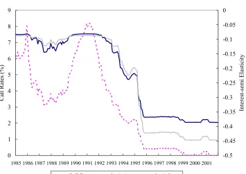
Next, we investigate the time profile of interest semi-elasticity using the
actual path of the call rate. Figure 4 illustrates the actual path of the call rate
and the path of the interest semi-elasticity. First, the interest semi-elasticity,
taking a value of about −0.07, had been quite stable until the early 1990s,
excluding the late 1980s, during which a low interest rate policy was temporarily
conducted. Second, as the call rate gradually lowered from a level of about
3%, interest semi-elasticity gradually increased from the early 1990s to the
mid-1990s. During the transition period, the interest semi-elasticity varies from−0.1
to−0.4. Third, in the period post-1995 when the BOJ guided the call rate below
0.5%, interest semi-elasticity took a larger value of about −0.45 and has been
quite stable.
The novelty of our finding is that we identify a transition period of interest
semi-elasticity from the early 1990s through to the mid-1990s. On the other
hand, for the period up until the early 1990s and for the period post-1995, our
estimates of interest semi-elasticity are compatible with existing empirical results
on the Japanese M1 demand function (Miyao, 2004; Fujiki and Watanabe, 2004;
Nakashima and Saito, 2006). Furthermore, compared with the existing empirical
results on US M1 demand, Japanese money demand is remarkably interest elastic
in the post-1995 period. 18
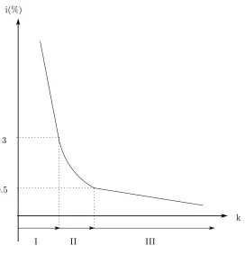
The above-mentioned results indicate that Japanese M1 demand is composed
of three regimes: Regimes I, II and III, as shown in Figure 5. In Regime I
money demand function had lower interest semi-elasticity. Regime II from the
early 1990s to the mid-1990s is the transition period during which the interest
semi-elasticity gradually changed. In Regime III from the mid-1990s, the policy
rate was set below 0.5%, and the Japanese money demand function had higher
interest semi-elasticity.
4
Conclusion
We have three substantive conclusions pertaining to the shape of the Japanese
money demand function. First, the linearity test showed that there is
statisti-cally significant evidence of nonlinearity in the semi-log money demand model,
whereas there is no comparable evidence pertaining to the double-log money
demand model. This result indicates that if we examine a semi-log model for
an extremely low interest rate economy similar to that in post-1995 Japan, we
must specifically consider the nonlinearity of interest semi-elasticity. On the
other hand, if we examine a double-log model, we can assume a conventional
linear specification.
Second, we confirmed that a semi-log money demand model has a
long-run equilibrium relationship with a nonlinear form. In addition, we provided
evidence that a nonlinear semi-log model is as effective as a linear double-log
model in terms of goodness-of-fit. Therefore, as long as we specifically introduce
nonlinearity, we can capture stable Japanese money demand, even with a
such as Fujiki and Watanabe (2004) and Bae, Kakkar, and Ogaki (2006) showed
the possibility of no-cointegration with a semi-log model and the inferiority of a
semi-log model to a double-log model without considering nonlinearity.
Third, we found that Japanese money demand comprises three regimes: the
first, through to the early 1990s, was when the Japanese money demand
func-tion had lower interest semi-elasticity; the second, from the early 1990s to the
mid-1990s, was when interest semi-elasticity gradually increased; and the third,
after the mid-1990s, was when the Japanese money demand function had higher
interest semi-elasticity.
In particular, with regard to the relationship between interest elasticity and
the BOJ’s policy rate, our estimation results indicate that it was when the BOJ
set the policy rate below 3% in the early 1990s that interest semi-elasticity began
to increase. As discussed by Lucas (2000), an interest rate of approximately 3%
would arise in the US economy under a policy of zero inflation. The finding
in the Japanese economy that even prior to 1999, when the BOJ started the
zero interest rate policy and the liquidity trap phenomenon became self-evident,
interest elasticity had already begun to increase would be beneficial in the actual
implementation of monetary policy.
Two aspects remain yet unaddressed in our empirical investigation. First,
we do not consider the relationship between the two competing models in the
cointegration analysis, that is, between a nonlinear semi-log model and a linear
smooth transition model. In particular, it is not yet understood whether each of
the competing models is nested or reduces to a unified model, especially if the
path of the short-term interest rate is monotonically falling as in Japan during
the 1990s. 19 Second, we exclude the period after 1999 or 2001 from our sample
because the inaction of nominal interest rates at their lower bound (0%) for
long-term periods (from 1999 to at least 2006) would cause serious econometric
problems. As pointed out by Elliott (1998), small amounts of mean reversion
that cannot be consistently determined by unit root tests render standard
coin-tegration inference highly misleading. If we include the sample period after 1999
to explicitly consider the zero bound, we must deal with this statistical problem
using a more rigorous time series method. We would like to extend our research
along these lines in the future.
Appendix: Simulation Methods and Results
A 1. Size and Power of the Linearity Test
To calculate the empirical power of the first-order (T1) and the third-order (T2)
tests, we generate data using the following system:
kt = constant1T +α1Tit+βT1it1−g(it;τT1)+ǫt (2)
it = it−1+vt (3)
ωt = s=p
s=1
Φsωt−s+ξt (4)
ξt ∼ i.i.d.N
¯
where (constant1T, α1T, βT1) andτT1 = (γT1, i∗1
T )′indicate the parameter estimates
obtained by the one-step Gauss–Newton estimator with a full sample of sizeT.
ωt is defined by ωt = (ǫt, vt)′. We calculate the empirical power through the
following steps:
1. Obtain the fitted residuals{ǫt:t= 1, . . . , T}in equation (2) using the
esti-matesθ1T, and define{vt:t= 1, . . . , T}in equation (3) by first differencing
the observed value of the call rate, that is,vt= ∆it.
2. Suppose that the data generating process ofωt= (ǫt, vt)′ :t= 1, . . . , T
is given by thep-th order vector autoregression (VAR), as shown by
equa-tion (4), to capture the regressor-error dependence. In addiequa-tion, estimate
the VAR by OLS to obtain the estimates{Φ1,Φ2, . . . ,Φp} and the fitted
VAR residuals {ξt:t=p+ 1, . . . , T}. The order is chosen based on the
Schwarz information criterion.
3. Draw a sample{ξ∗
t} of sizeT +p from the normal distribution (5) with a mean ¯ξ = T1 T
t=1ξt and a varianceσ2 = T1
T
t=1
ξt−ξ¯2.
4. Generate a sampleω∗
t = (ǫ∗t, vt∗) ′
:t= 1, . . . , Trecursively, using the
es-timated VAR, and obtain a sample{i∗t;t= 1, . . . , T}of the call rate by
in-tegratingv∗
t, that is,i∗t =i0+tj=1vj∗, wherei0 indicates the initial value ofit. In addition, generate a sample{k∗
t :t= 1, . . . , T} of the Marshallian kby substituting the residualsǫ∗
estimator.
5. Apply the first-order and third-order tests for linearity based on the 5%
asymptotic critical values to each set of the sample (k∗
t, i∗t), and repeat this procedure 5,000 times.
Table A-1 reports rejection frequencies from Monte Carlo studies of the power
of the linearity tests. As shown in each panel of Table A-1, the calculated power
does not seriously deteriorate.
Next, we calculate the size of the linearity tests as follows. Assuming that
βT1 = 0 under the null of linearity, we obtain the fitted residuals by using the
estimates (constant1
T, α1T)′. Then, we follow the same procedure as in the cal-culation of power. Table A-1 reports the rejection frequencies under the null
hypothesis as the size of the linearity tests. In the two sample periods, neither
shows substantial over rejection.
The Monte Carlo studies demonstrate that the test results based on our
sample do not suffer from serious small sample biases.
A 2. Size and Power of the Nonlinear Cointegration Test
To examine the small sample properties of Choi and Saikkonen’s (2005) Cθ1
T
test for cointegration, we alter the Monte Carlo procedure for the linearity test
as follows. First, we assume that a cointegrating error ǫt can be described as
follows:
wt ∼ i.i.d.Nw, σ¯ w2. (7)
Furthermore, we assume ρ = 0 under the null hypothesis and ρ = 0 under the
alternative hypothesis. On calculation of size, we estimate AR(1) process (6)
using the fitted residuals{ǫt}, obtained in step 1 of the Monte Carlo procedure
for the linearity test, whereas in the calculation of power, we first consider the
difference of the fitted residuals. Then, we obtain a sample of{wt:t= 1, . . . , T}.
Second, we assume that the sample {wt} follows an i.i.d. normal distribution
(7) with a mean ¯w = T1 T
t=1wt and a variance σw2 = T1
T
t=1(wt−w¯)2, and generate a sample {w∗
t} of size T + 1 from the normal distribution. Third, we obtain a sample {ǫ∗
t;t= 1, . . . , T} by integrating w∗t. Except for using the generated cointegrating errors {ǫ∗
t}, we follow the same procedure as for the
linearity test in calculating both size and power.
Table A-2 reports the calculated size and power of theCθ1
T test. Overall, the
Cθ1
T test shows good small sample performance. For the size, the test reveals no
serious size distortion. The empirical power is also reasonably high.
A 3. Comparative Simulation Study of the Two Models
To conduct a comparative simulation study of the linear double-log and nonlinear
semi-log models, we alter the Monte Carlo procedure for the linearity test as
follows. First, when we adopt the linear double-log model as the true model, it
indicates a logarithmic value of the overnight call rate in the system given by (2)–
fully modified OLS in Phillips and Hansen (1990). Second, when we adopt the
nonlinear semi-log model as the true model, we estimate (constant1T, α1T, βT1)
and τ1
T = (γT1, i∗T1)′ using the two-step Gauss–Newton estimator with K = 1 and not using the one-step Gauss–Newton estimator. Third, to prepare for the
out-of-sample prediction experiments for the periods up to 2001/I, and up to
2002/IV, we estimate the parameters of the true model using the sample from
1985/I to 2001/I, and from 1985/I to 2002/IV, respectively. Fourth, in step 5,
we use the sample (k∗
t, i∗t) obtained by simulating a draw for the true model, thereby calculating a simulated sum of squared error for the other. We repeat
this procedure 1,000 times to obtain the mean of simulated sums of squared
error: e∗. We calculate the mean square error (MSE) and bias (BIAS) defined
as (e−e∗)2 and e−e∗, where e indicates an empirical sum of squared error
presented by Table 3.
According to Table 4, the MSE and the BIAS of the nonlinear semi-log model
are smaller than those of the linear double-log model. For the in-sample
predic-tion, the double-log model partly exceeds the nonlinear semi-log model, while
for the out-of-sample prediction, the nonlinear semi-log model largely exceeds
the double-log model in all of the prediction periods.
A 4. Bootstrap Confidence Interval
To obtain bootstrap confidence intervals, we alter the Monte Carlo procedure
obtained by the one-step and two-step Gauss–Newton estimators with K =
1,2,4. Second, in step 3, we sample ξ∗
t of size T randomly with replacement from the centered VAR residuals
ξt−ξ¯:t= 1, . . . , T
, where ¯ξ = T1 T t=1ξt. Third, in step 5, we calculate the confidence interval based on the one-step and
the two-step Gauss–Newton estimators by using the bootstrap sample obtained
in step 4. Except for these steps, we follow the same procedure as the linearity
tests in calculating power.
According to Table 5, while the estimated confidence intervals are somewhat
larger than those based on asymptotic distribution, the sign and significance of
the estimated parameters do not change substantially.
Footnotes
1 As an exception, Hondroyiannis, Swamy, and Tavlas (2000) employed a random
coefficient model and found that the absolute value of the interest elasticity
esti-mate continuously decreased, even in the lower interest rate period. Their finding
should, however, be reserved because it is not clear that the random coefficient
model can be applied when dealing with the coefficients of integrated variables.
2 Miyao (2004) and Fujiki and Watanabe (2004) have shown that Gregory and
Hansen’s (1996) cointegration test, which allows for a possible structural break
in a linear context, detected cointegration with a double-log model but not with a
semi-log model. In contrast, Miyao (2004) showed that the Johansen (1988) and
Johansen and Juselius (1990) cointegration tests detected cointegration with both
ordinary least squares (OLS) or dynamic OLS, Bae et al. (2006) used the
non-linear cointegration technique in Bae and de Jong (2007) to estimate a double-log
money demand function, thereby dealing with the statistical issue of the nonlinear
transformation of interest rates as the I(1) variable. Their finding for out-of-sample
prediction performance did not depend on the techniques used for their estimation.
4 Cagan (1956) devised a semi-log money demand model to analyze hyperinflation.
Nakashima and Saito (2006) developed a semi-log money demand model based
on the classical Cagan model to examine deflation in Japan in the late 1990s.
Lagos and Wright (2005) derived a semi-log model employing a search-theoretical
approach. Conversely, the double-log money demand model mainly derives its
theoretical background from new classical representative agent models, including
the shopping-time model (see McCallum and Goodfriend (1989), and Lucas (1988,
2000)).
5 Lucas (2000) demonstrated that the estimated welfare cost of inflation varies
de-pending on which of the two models is used. Miyao (2004) reviews recent
devel-opments in liquidity trap theories.
6 Applications of the smooth transition model for modeling the money demand
equa-tion include Wolters, Ter¨asvirta, and L¨utkepohl (1998), L¨utkepohl, Ter¨asvirta, and
Wolters (1999), Sarno (1999), Huang, Lin, and Cheng (2001), and Ter¨asvirta and
Eliasson (2001). Unlike the present paper, these studies all assume a linear long-run
relation between money and other variables that is based on economic theories for
money demand, thus using a smooth transition error correction model to capture
nonlinear dynamics of a short-run correction process to a long-run equilibrium.
7 Christopoulos and Le´on-Ledesma (2007) have applied Saikkonen and Choi’s (2004)
They do not model the short-run error correction dynamics to the long-run
equi-librium.
8 In contrast, a structural break model is a simple time-dependent parameter model.
Hence, the structural break model is not appropriate for estimating the time
pro-file of a parameter coefficient in relation to an explanatory variable of concern.
Furthermore, the structural break model cannot identify the transition value, even
though the model can identify the change point at which the set of coefficient
parameters change.
9 Fujiki and Watanabe (2004) provide evidence that the estimates of income
elastic-ity lie close to unelastic-ity. Nakashima and Saito (2006) found that the income elasticelastic-ity
for Japanese money demand was stable over time with the partial structural change
test of Kuo (1998). Miyao (2004) and Bae, Kakkar, and Ogaki (2006) adopted the
velocity-based specification for modeling the Japanese money demand function.
We follow these studies to form a base specification for the Japanese money
de-mand function.
10 There is a long controversy over which short- or long-term rate should be included
in the empirical specification of the money demand equations as the opportunity
cost of holding money (e.g., Poole, 1988; Hoffman and Rasche, 1991). Hoffman,
Rasche, and Tieslau (1995), however, argued that if two interest rates are
cointe-grated from the term structure, the interest rate used is irrelevant to the estimates
of interest elasticity. Indeed, they employed the overnight call rate as the most
representative short-term rate in Japan. Accordingly, we employ the call rate not
only as the BOJ’s policy indicator, but also as the opportunity cost of holding
up to February 2001 and that an equally weighted average of the call rate and
reserves represented the BOJ’s policy decisions from March 2001.
12 The NLLS estimator θT is consistently of the orderOp(T− 1
2), which differs from
Op(T−1) obtained in the linear cointegrating cases.
13 More specifically, the algorithm of the minimum volatility rule is as follows. First,
for each b = bsmall to b = bbig, we compute a statistical value C(b). Next, for
eachb, we calculate the standard deviation of C(b−m), . . . , C(b+m), where m
denotes an integer ofm≥1. Lastly, we pick the valueb∗with the smallest standard
deviation and reportC(b∗) as the final statistical value.
14 Choi and Saikkonen (2005) give the cumulative distribution function of1
0 w
2 (r)dr
as
F(z) =√2 ∞
n=0
Γ(n+ 1/2)
n!Γ(1/2) (−1)
n
1−f
u
2√z
, z≥0,
wheref(x) = 2
√π0xexp(−β)dβandu= √
2
2 + 2n
√
2. zindicates test statistics for
the cointegration test. Choi and Saikkonen (2005) suggest truncating the series at
n= 10.
15 We also conducted the linearity test for income elasticity without imposing unitary
income elasticity. We have strong evidence pertaining to the linearity of income
elasticity.
16 For the performance comparison of out-of-sample prediction, Bae et al. (2006)
also used a nonlinear model implied by the money in the utility function with
the constant elasticity of substitution. They showed that the nonlinear model
displayed similar performance to the double-log model.
17 The estimation results for the sample periods from 1980/I are similar to those for
18 Stock and Watson (1993) applied several estimation methods to the sample period
1946–1987 and found that the estimated interest semi-elasticity ranged from−0.02
to−0.09. By extending the postwar US data through to 1996, Ball (2001)
demon-strated that the interest semi-elasticity was approximately−0.05. From existing
empirical work on US M1 demand, we cannot find any point estimates of interest
semi-elasticity around−0.4 or−0.5.
19 Bae and de Jong (2007) developed a nonlinear cointegration technique to estimate
a double-log model, thereby rigorously modeling the nonlinearity of interest
semi-elasticity using the double-log model. Carrasco (2002) studied the relationships
between a structural change model, a threshold model, and a Markov-switching
model. Her study, however, only concerns the modeling of stationary variables.
References
[1] Andrews, D., 1991, Heteroskedasticity and Autocorrelation Consistent Covariance
Ma-trix Estimator, Econometrica, 59, 817–858.
[2] Bae, Y., and De Jong, R., 2007, Money Demand Function Estimation by Nonlinear
Cointegration, Journal of Applied Econometrics, 22, 767–793.
[3] Bae, Y., Kakkar, V., and Ogaki, M., 2006, Money Demand in Japan and Nonlinear
Cointegration, Journal of Money, Credit and Banking, 38, 1659–1668.
[4] Ball, L., 2001, Another Look at Long-run Money Demand, Journal of Monetary
Eco-nomics, 47, 31–44.
[5] Cagan, P., 1956, The Monetary Dynamics of Hyperinflation, inStudies in the Quantity
[6] Carrasco, M., 2002, Misspecified Structural Change, Threshold, and Markov-switching
Models, Journal of Econometrics, 109, 239–273.
[7] Dickey, D., and Fuller, W., 1979, Distribution of the Estimators for Autoregressive Time
Series with a Unit Root, Journal of the American Statistical Association, 74, 427–431.
[8] Chang, Y., Park, J., and Phillips, P., 2001, Nonlinear Econometric Models with
Coin-tegrated and Deterministically Trending Regressors, Econometrics Journal, 4, 1–36.
[9] Choi, I., and Saikkonen, P., 2004, Testing Linearity in Cointegrating Smooth Transition
Regressions, Econometrics Journal, 7, 341–365.
[10] Choi, I., and Saikkonen, P., 2005, Test for Nonlinear Cointegration, mimeo.
[11] Christopoulos, D., and Le´on-Ledesma, M., 2007, A Long-run Nonlinear Approach to
the Fisher Effect, forthcoming in Journal of Money, Credit and Banking.
[12] Elliott, G., 1998, On the Robustness of Cointegration Methods when Regressors Almost
Have Unit Roots, Econometrica, 66, 149–158.
[13] Fujiki, H., and Watanabe, K., 2004, Japanese Demand for Narrow Monetary Aggregate
in the 90s: Time Series versus Cross-sectional Evidence from Japan, Monetary and
Economic Studies, 22, 47–77.
[14] Gregory, A., and Hansen, B., 1996, Residual-based Tests for Cointegration in Models
with Regime Shifts, Journal of Econometrics, 70, 99–126.
[15] Hansen, B., 1992, Tests for Parameter Instability in Regressions Analysis with I(1)
Processes, Journal of Business and Economic Statistics, 10, 321–335.
[16] Hoffman, D., and Rasche, R., 1991, Long-run Income and Interest Elasticities of Money
[17] Hoffman, D., Rasche, R., and Tieslau, M., 1995, The Stability of Long-run Money
Demand in Five Industrial Countries, Journal of Monetary Economics, 35, 317–339.
[18] Hondroyiannis, G., Swamy, P.A.V.B., and Tavlas, G., 2000, Is the Japanese Economy
in a Liquidity Trap?, Economic Letters, 66, 17–23.
[19] Huang, H., Lin, J., and Cheng, J., 2001, Evidence on Nonlinear Error Correction in
Money Demand: The Case of Taiwan, Applied Economics, 33, 1727–1736.
[20] Johansen, S., 1988, Statistical Analysis of Cointegrating Vectors, Journal of Economic
Dynamic and Control, 12, 213–254.
[21] Johansen, S., and Juselius, K., 1990, Maximum Likelihood Estimation and Inference
on Cointegration—With Application to the Demand for Money, Oxford Bulletin of
Economics and Statistics, 52, 169–210.
[22] Kuo, B., 1998, Test for Partial Parameter Instability in Regressions with I(1) Processes,
Journal of Econometrics, 86, 337–368.
[23] Kwiatkowski, D., Phillips, P., Schmidt, P., and Shin, Y., 1992, Testing the Null
Hy-pothesis of Stationarity against the Alternative of a Unit Root: How Sure Are We That
Economic Time Series Have a Unit Root?, Journal of Econometrics, 54, 159–178.
[24] Lagos, R., and Wright, R., 2005, A Unified Framework for Monetary Theory and Policy
Analysis, Journal of Political Economy, 113, 463–484.
[25] Lucas, R., 1988, Money Demand in the United States: A Quantitative Review,
Carnegie–Rochester Conference Series on Public Policy, 29, 137–168.
[26] Lucas, R., 2000, Inflation and Welfare, Econometrica, 68, 137–168.
[27] L¨utkepohl, H., Ter¨asvirta, T., and Wolters, J., 1999, Investigating Stability of Linearity
[28] McCallum, B., and Goodfriend, M., 1989, Demand for Money: Theoretical Studies, in
The New Palgrave Dictionary of Economics: Money, ed. Eatwell, J., Milgate, M., and
Newman, P., New York: W.W. Norton.
[29] Miyao, R., 2004, Liquidity Traps and the Stability of Money Demand: Is Japan Really
Trapped at the Zero Bound?, Mimeo, Kobe University.
[30] Nakashima, K., 2006, Ideal and Real Japanese Monetary Policy: A Comparative
Analy-sis of Actual and Optimal Policy Measures, forthcoming in Japanese Economic Review.
[31] Nakashima, K., and Saito, M., 2006, Uncovering Interest-elastic Money Demand:
Evi-dence from the Japanese Money Market with a Low Interest Rate Policy, Mimeo,
Hi-totsubashi University.
[32] Park, J., and Phillips, P., 1999, Asymptotics for Nonlinear Transformations of Time
Series, Econometric Theory, 15, 269–298.
[33] Park, J., and Phillips, P., 2001, Nonlinear Regressions with Integrated Time Series,
Econometrica, 69, 117–161.
[34] Phillips, P., and Hansen, B., 1990, Statistical Inference in Instrumental Variables
Re-gression with I(1) Processes, Review of Economic Studies, 57, 99–125.
[35] Phillips, P., and Perron, P., 1988, Testing for a Unit Root in Time Series Regression,
Biometrika, 75, 335–346.
[36] Poole, W., 1988, Monetary Policy Lessons of Recent Inflation and Deflation, Journal of
Economic Perspectives, 2, 51–72.
[37] Romano, J., and Wolf, M., 2001, Subsampling Intervals in Autoregressive Models with
[38] Saikkonen, P., 2005, Stability Results for Nonlinear Error Correction Models, Journal
of Econometrics, 127, 69–81.
[39] Saikkonen, P., 2008, Stability of Regime Switching Error Correction Models under
Lin-ear Cointegration, Econometric Theory, 24, 294–318.
[40] Saikkonen, P., and Choi, I., 2004, Cointegrating Smooth Transition Regressions,
Econo-metric Theory, 20, 301–340.
[41] Sarno, L., 1999, Adjustment Costs and Nonlinear Dynamics in the Demand for Money:
Italy, 1861–1991, International Journal of Finance and Economics, 4, 155–177.
[42] Stock, J., and Watson, M., 1993, A Simple Estimator of Cointegrating Vectors in Higher
Order Integrated Systems, Econometrica, 61, 783-820.
[43] Ter¨asvirta, T., and Eliasson, A., 2001, Nonlinear Error Correction and the UK Demand
for Broad Money, 1878–1993, Journal of Applied Econometrics, 16, 277–288.
[44] Wolters, J., Ter¨asvirta, T., and L¨utkepohl, H., 1998, Modelling the Demand for M3 in
Table 1: Test Results for Cointegration with Possible Nonlinearity
Double-log Model
Period
Cθ1
T
Cθ T
K= 1 K= 2 K= 4
1980/I–2001/I
P-value 0.638 0.654 0.706 0.654 (0.440) (0.464) (0.553) (0.465) Block Size 24 23 24 46
1985/I–2001/I
P-value 0.598 0.772 0.801 0.764 (0.387) (0.705) (0.794) (0.685) Block Size 35 48 21 16
1980/I–1999/I
P-value 0.874 0.688 0.765 0.601 (1.586) (0.520) (0.687) (0.390) Block Size 59 36 59 38
1985/I–1999/I
P-value 0.628 0.822 0.801 0.103 (0.426) (0.879) (0.797) (0.092) Block Size 16 37 35 39
Semi-log Model
Period
Cθ1
T
Cθ T
K= 1 K= 2 K= 4
1980/I–2001/I
P-value 0.741 0.765 0.701 0.410 (0.628) (0.686) (0.544) (0.214) Block Size 51 51 49 77
1985/I–2001/I
P-value 0.727 0.758 0.667 0.224 (0.596) (0.667) (0.484) (0.128) Block Size 29 52 27 52
1980/I–1999/I
P-value 0.603 0.588 0.665 0.643 (0.392) (0.374) (0.482) (0.447) Block Size 65 30 45 49
1985/I–1999/I
P-value 0.541 0.641 0.725 0.185 (0.321) (0.445) (0.593) (0.128) Block Size 46 41 11 47 1. Cθ
T and Cθ1
T
denote the cointegration tests based on the NLLS estimation and the one-step Gauss–Newton estimation, respectively.
2. Kdenotes the number of leads and lags in the regression model.
3. P-values are calculated using the cumulative distribution function in Choi and Saikkonen (2005). 4. Test statistics are reported in parentheses.
5. Block sizes are calculated using the minimum variance rule withm= 2.
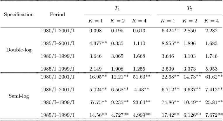
Table 2: Linearity Tests for the Japanese Money Demand Function
Specification Period
T1 T2
K= 1 K= 2 K= 4 K= 1 K= 2 K= 4
Double-log
1980/I–2001/I 0.398 0.195 0.613 6.424** 2.850 2.282
1985/I–2001/I 4.377** 0.335 1.110 8.255** 1.896 1.683
1980/I–1999/I 3.646 3.065 1.668 3.646 3.103 1.746
1985/I–1999/I 2.149 1.908 1.255 2.539 3.373 5.953
Semi-log
1980/I–2001/I 16.95** 12.21** 51.63** 22.68** 14.73** 61.62**
1985/I–2001/I 5.024** 6.568** 4.43** 6.712** 9.637** 7.412**
1980/I–1999/I 57.75** 9.235** 23.64** 74.86** 10.49** 25.81**
1985/I–1999/I 14.56** 4.727** 4.999** 17.42** 6.126** 7.672**
1. Kdenotes the number of leads and lags in the regression model. 2. * and ** indicate the significance levels of 5% and 10%, respectively.
3. T1andT2 have the asymptotic distributions with degrees of freedom one and two, respectively.
Table 3: Test Results for Goodness-of-fit
Model
In-sample Prediction Out-of-sample Prediction
1985/I-1999/I 1985/I-2001/I 1980/I-2001/I 1998/II-2001/I 1999/II-2001/I 1999/II-2002/IV
Linear Semi-log 0.381 1.029 2.987 0.867 0.475 1.225
Linear Double-log 0.081 0.367 0.431 0.345 0.403 0.611
Nonlinear Semi-log 0.094 0.230 0.356 0.449 0.025 0.295
Nonlinear Double-log 0.373 7.620 7.854 16.85 1.827 3.886
1. The table reports the sum of squares error (SSE) of the in-sample and out-of-sample prediction. 2. The SSEs of the out-of-sample prediction for the periods from 1998/II, and from 1999/II are based on estimates using the sample from 1985/I to 1998/I, and from 1985/I to 1999/I, respectively.
3. We calculate the SSEs for the linear semi-log and double-log models by performing the fully modified OLS estimation in Phillips and Hansen (1990).
Table 4: Comparative Simulation Study of the Linear Double-log and Nonlinear Semi-log Models
In-sample Prediction
True Model
Prediction Period
1985/I-1999/I 1985/I-2001/I 1980/I-2001/I
Linear Double-log
MSE 1.138 0.317 0.913
BIAS -1.177 -0.563 -0.956
Nonlinear Semi-log
MSE 0.301 0.414 1.928
BIAS -0.548 -0.643 -1.388
Out-of-sample Prediction
True Model
Prediction Period
1998/II-2001/I 1999/II-2001/I 1999/II-2002/IV
Linear Double-log
MSE 0.881 0.783 10.86
BIAS -0.939 -0.884 -3.295
Nonlinear Semi-log
MSE 0.006 0.012 0.005
BIAS -0.079 0.110 0.068
1. The table reports the simulated mean square error (MSE) and bias (BIAS) of the SSEs presented in Table 3. The MSE and the BIAS are defined as (e−e∗)2ande−e∗, whereeande∗indicate
an empirical SSE presented in Table 3 and the mean of the SSEs obtained using Monte Carlo simulation.
2. When the linear double-log model (the nonlinear semi-log model) is adopted as the true model, the MSE and the BIAS are obtained by simulating draws from the true model and estimating a SSE of the nonlinear semi-log model (the linear double-log model) for each draw.
Table 5: Parameter Estimates of Nonlinear Money Demand Model
Period I (1985/I–1999/I)
Estimation K C.I. α β γ i∗
One-step 1
-0.049 -0.219 0.756 3.246 Asy (-0.070, -0.027) (-0.362, -0.076) (0.369, 1.144) (1.050, 5.442) Boot (-0.055, -0.040) (-0.319, -0.185) (0.667, 0.822) (2.778, 3.628)
2
-0.048 -0.213 0.752 3.253 Asy (-0.075, -0.021) (-0.381, -0.044) (0.329, 1.176) (0.750, 5.757) Boot (-0.055, -0.037) (-0.329, -0.175) (0.659, 0.823) (2.732, 3.673)
4
-0.043 -0.217 0.743 3.136 Asy (-0.080, -0.007) (-0.437, 0.004) (0.240, 1.247) (0.106, 6.166) Boot (-0.053, -0.029) (-0.361, -0.168) (0.638, 0.829) (2.526, 3.641)
Two-step 1
-0.069 -0.204 0.872 3.144 Asy (-0.152, 0.014) (-0.719, 0.312) (-0.213, 1.957) (-0.593, 6.880) Boot (-0.105, -0.027) (-0.601, -0.055) (0.583, 1.137) (2.201, 4.044)
2
-0.070 -0.198 0.879 3.144 Asy (-0.156, 0.015) (-0.719, 0.323) (-0.234, 1.992) (-0.750, 7.039) Boot (-0.106, -0.028) (-0.596, -0.034) (0.565, 1.144) (2.076, 4.037)
4
-0.068 -0.202 0.887 2.989 Asy (-0.171, 0.353) (-0.835, 0.432) (-0.502, 2.276) (-1.769, 7.747) Boot (-0.117, -0.017) (-0.661, -0.007) (0.500, 1.242) (1.713, 4.170)
Period II (1985/I–2001/I)
Estimation K C.I. α β γ i∗
One-step 1
-0.081 -0.342 1.142 1.868 Asy (-0.099, -0.063) (-0.520, -0.164) (0.298, 1.985) (0.242, 3.493) Boot (-0.091, -0.069) (-0.449, -0.225) (0.873, 1.338) (1.358, 2.333)
2
-0.083 -0.303 1.049 2.109 Asy (-0.103, -0.063) (-0.501, -0.105) (0.152, 1.945) (0.338, 3.880) Boot (-0.098, -0.078) (-0.468, -0.261) (0.886, 1.368) (1.796, 2.716)
4
-0.087 -0.206 0.754 2.727 Asy (-0.115, -0.059) (-0.496, 0.085) (-0.362, 1.869) (0.396, 5.059) Boot (-0.103, -0.082) (-0.339, -0.176) (0.602, 1.078) (2.435, 3.400)
Two-step 1
-0.087 -0.397 1.458 1.566 Asy (-0.139, -0.035) (-0.957, 0.163) (-0.644, 3.560) (-1.132, 4.265) Boot (-0.132, -0.074) (-0.901, -0.223) (0.838, 2.142) (0.791, 2.422)
2
-0.089 -0.305 1.242 1.995 Asy (-0.131, -0.047) (-0.688, 0.077) (-0.012, 2.495) (-0.052, 4.041) Boot (-0.117, -0.075) (-0.596, -0.204) (0.917, 1.605) (1.499, 2.574)
4
-0.086 -0.118 0.743 3.383 Asy (-0.165, -0.007) (-0.658, 0.422) (-0.585, 2.071) (-0.861, 7.627) Boot (-0.117, -0.072) (-0.403, -0.057) (0.543, 0.943) (2.780, 3.996) 1. One-step and Two-step denote the one-step and two-step Gauss–Newton estimations,
respec-tively.
2. Kdenotes the number of leads and lags in the regression model.
3. The number in parentheses denotes the 95% confidence interval. To calculate the 95% confidence interval, we use the long-run variance estimated through Andrews’ (1991) method with an AR(4) approximation for the prefilter.
Table A-1: Empirical Size and Power of Linearity Tests
Period I (1985/I–1999/I)
Specification
T1 T2
K= 1 K= 2 K= 4 K= 1 K= 2 K= 4
Double-log
Size 0.100 0.120 0.156 0.082 0.092 0.130
Power 0.781 0.832 0.997 0.744 0.803 0.927
Semi-log
Size 0.091 0.094 0.125 0.059 0.063 0.079
Power 0.754 0.750 0.760 0.732 0.717 0.744
Period II (1985/I–2001/I)
Specification
T1 T2
K= 1 K= 2 K= 4 K= 1 K= 2 K= 4
Double-log
Size 0.103 0.154 0.230 0.087 0.122 0.293
Power 0.547 0.698 0.851 0.464 0.583 0.868
Semi-log
Size 0.134 0.149 0.215 0.089 0.106 0.169
Power 0.864 0.869 0.846 0.851 0.868 0.847
1. Data are generated as discussed in the Appendix.
2. Kdenotes the number of leads and lags in the regression model.
3. Empirical size is calculated under the null of linearity (β= 0), and empirical power is calculated under the alternative of nonlinearity (β= 0).
4. The number of iterations is 5,000 and the nominal size is 5%.
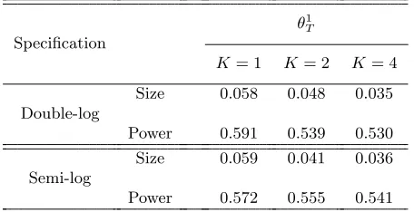
Table A-2: Empirical Size and Power of the Nonlinear Cointegration Test
Period I (1985/I–1999/I)
Specification
θ1 T
K= 1 K= 2 K= 4
Double-log
Size 0.055 0.061 0.054
Power 0.437 0.406 0.401
Semi-log
Size 0.056 0.060 0.050
Power 0.439 0.417 0.404
Period II (1985/I–2001/I)
Specification
θ1 T
K= 1 K= 2 K= 4
Double-log
Size 0.058 0.048 0.035
Power 0.591 0.539 0.530
Semi-log
Size 0.059 0.041 0.036
Power 0.572 0.555 0.541
1. Data are generated as discussed in the Appendix.
2. Kdenotes the number of leads and lags in the regression model.
3. Empirical size is calculated under the null of cointegration and empirical power is calculated under the alternative of no-cointegration.
4. The number of iterations is 5,000 and the nominal size is 5%.
Figure 1. Overnight Call Rates and Marshallian k
0% 2% 4% 6% 8% 10% 12% 14%
19801981198219831984198519861987198819891990199119921993199419951996199719981999200020012002200320042005
0 1 2 3 4 5 6 7 8
Figure 2: Semi-log Model and Double-log Model (1985/I-2001/I)
Semi-log Model
0 1 2 3 4 5 6 7 8 9
2 2.5 3 3.5 4 4.5 5
Marshallian k (=M1/GDP)
Call Rates (%)
Double-log Model
-2.5 -2 -1.5 -1 -0.5 0 0.5 1 1.5
2 2.5 3 3.5 4 4.5 5
Marshallian k (=M1/GDP)
Figure 3. Level of Nominal Interest Rates and Interest Semi-elasticity
-0.5 -0.45 -0.4 -0.35 -0.3 -0.25 -0.2 -0.15 -0.1 -0.05 0
14% 13% 12% 11% 10% 9% 8% 7% 6% 5% 4% 3% 2% 1%
Interest-semi Easticity
k=1, 1step k=1, 2step
Figure 4. Time Profile of Interest Semi-elasticity
0 1 2 3 4 5 6 7 8 9
1985 1986 1987 1988 1989 1990 1991 1992 1993 1994 1995 1996 1997 1998 1999 2000 2001
Call Rates (%)
-0.5 -0.45 -0.4 -0.35 -0.3 -0.25 -0.2 -0.15 -0.1 -0.05 0 Interest-semi Elasticity
[image:48.595.142.497.458.709.2]Figure 5. The Shape of the Japanese Money Demand Function
i(%)
k 3
0.5