Inferential framework for nonstationary dynamics II Application to a model of physiological signaling

Inferential framework for nonstationary dynamics. II. Application to a model

of physiological signaling

Andrea Duggento,1Dmitri G. Luchinsky,1,2,3Vadim N. Smelyanskiy,2 Igor Khovanov,1and Peter V. E. McClintock1 1

Department of Physics, Lancaster University, Lancaster LA1 4YB, United Kingdom 2

NASA Ames Research Center, Mail Stop 269-2, Moffett Field, California 94035, USA 3

Mission Critical Technologies, Inc., 2041 Rosecrans Avenue, Suite 225, El Segundo, California 90245, USA 共Received 30 January 2008; published 4 June 2008兲

The problem of how to reconstruct the parameters of a stochastic nonlinear dynamical system when they are time-varying is considered in the context of online decoding of physiological information from neuron signal-ing activity. To model the spiksignal-ing of neurons, a set of FitzHugh-Nagumo 共FHN兲 oscillators is used. It is assumed that only a fast dynamical variable can be detected for each neuron, and that the monitored signals are mixed by an unknown measurement matrix. The Bayesian framework introduced in paper I 共immediately preceding this paper兲is applied both for reconstruction of the model parameters and elements of the measure-ment matrix, and for inference of the time-varying parameters in the nonstationary system. It is shown that the proposed approach is able to reconstruct unmeasured共hidden兲slow variables of the FHN oscillators, to learn to model each individual neuron, and to track continuous, random, and stepwise variations of the control parameter for each neuron in real time.

DOI:10.1103/PhysRevE.77.061106 PACS number共s兲: 02.50.Tt, 05.45.Tp, 05.10.Gg, 05.45.Xt

I. INTRODUCTION

Time variability and nonlinearity are natural ingredients of physiological systems. In addition, a system’s environ-ment and its own internal complexity often create a strong fluctuational background that is frequently an essential fea-ture of the dynamics. It is a context where physiological models are rarely known from first principles, and model identification and parameter inference become indispensable from the points of view of both fundamental and applied physiology关1,2兴and in view of likely medical applications. In many situations, the real-time tracking of physiological parameters is the key to successful applications including, e.g., brain-controlled interfaces关3,4兴. However, the interplay of noise, nonlinearity, and the time variability of the model parameters makes it difficult to extract reliable information from the data, and very difficult to do so quickly. Accord-ingly, the simplifying assumptions of linearity and/or deter-minism关2,5兴are frequently made in an attempt to facilitate inference rather than on physiological grounds.

In addition, physiologically important parameters that de-scribe specific features of the system state or system dynam-ics are not usually directly measurable and have to be in-ferred from measurements of other types of information. At present, there are no general methods available to solve this problem if the model is stochastic, nonlinear, and nonstation-ary, i.e., its parameters vary in time.

In paper I 关6兴, we introduced a general Bayesian frame-work that allows one to identify a nonlinear stochastic model from time-series data and to infer its time-varying parameters in real time. In the present paper, we verify the approach by applying it to the analysis of a model of physiological sig-naling. The model chosen is a set of the FitzHugh-Nagumo 共FHN兲systems 关7–9兴. It has been found useful in analyzing

dynamics of nerve fibers 关10兴 and certain muscle cells in heart tissue关11–13兴. It has also been used intensively in

stud-ies of passive myelinated axons 关14兴 and various forms of

arrythmia and cardiac activation evolution关15兴. The control

of such neural-related dynamics is important in the context of biotechnological applications ranging from neural models of voluntary movement 关16兴 to studies of control in nerve conduction关17兴.

In our model, the measured signals corresponding to fast variables of the FHN system 共e.g., action potentials兲 are mixed by the unknown measurement matrix. Slow variables are hidden, which is the case in most real applications. It is assumed that physiological information is coded in the time-varying control parameters␩of each FHN system. Our goals will be to reconstruct the hidden variables and the measure-ment matrix, to learn the parameters of each individual sys-tem, and to use this information for extracting the time varia-tion of the control parameter␩in real time. We will show, in particular, that the approach is able to decode large stepwise changes, as well as random and continuous variations of the control parameter, for each oscillator in real time. Further-more, we will show that the parameter-tracking algorithm can effectively be embedded into the inferential learning framework, enabling us to reconstruct both the unmeasured 共hidden兲variables of the FHN oscillators and the model pa-rameters. For simplicity, we will assume that FHN systems are not coupled and that the dynamical equation for the slow variable does not include a random force. However, both coupling and noise in the hidden variables can be incorpo-rated into the method, as will be shown elsewhere.

II. SYSTEM OF FITZHUGH-NAGUMO OSCILLATORS

In a typical physiological situation, neurons fire at the rate of⬃5 – 10 s−1_{. The correlation time of the control parameter}

is⬃500– 1000 ms. The correlation times of other model

pa-rameters in the nonstationary case are ⬃5 s. A typical sam-pling rate for measurements is⬃20 kHz. In order to follow the time variations, it is necessary for the computation time to be less than the shortest characteristic time in the system, i.e., that for variation of the control parameters. So we must aim for a computational inference delay time of less than 500 ms.

To model this spiking activity, we use the well-known FitzHugh-Nagumo system in the form

v˙j= −vj共vj−␣j兲共vj− 1兲−qj+␩j+

冑

Dji␰i,

q˙j= −␤qj+␥jvj,

具␰j共t兲␰i共t

⬘兲典

=␦ij␦共t−t

⬘兲,

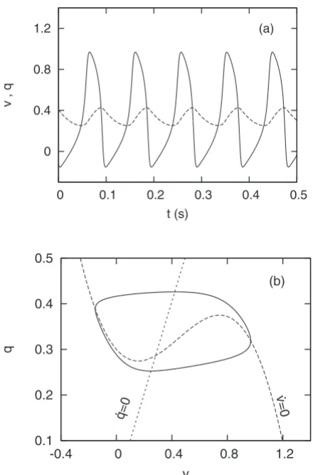
j= 1:L. 共1兲 This system共1兲represents the simplified dynamics ofL non-interacting neurons 关8兴, where vj model the membrane po-tentials and qj are slow recovery variables. Figure 1

illus-trates the dynamics for one oscillator in the absence of noise; values of the other parameters are ␣= 0.4, ␩= 0.3, ␤ = 0.0151, and␥= 0.0153.

We assume that the important physiological information is encoded in the parameters␩i, which control the frequency of firing. In practice, this information is difficult to extract be-cause signals collected from biological systems are noisy and often mixed with an unknown measurement matrix. To ana-lyze the situation in a realistic way, we introduce dynamical noise into the model system共1兲and a measurement matrixX into the following measurement model:

yi=Xijvj. 共2兲

Hereyiare measured variables, related tovjby linear trans-formation with theunknownmatrixX. An example of noisy signals before and after the mixing is shown in Fig. 2. We suppose that the only accessible information is contained in yi. The problem is therefore to learn the model parameters M=兵␩i,␣i,qi共0兲,␥i,Dij,Xij其 from the time-series data 兵yi其, and to use this information for fast on-line tracking of the time-varying parameters兵␩i其 for each neuron. It was shown in paper I that this problem can be treated within a general inferential framework by integrating the middle set of equa-tions in Eqs.共1兲to obtain

qj共t兲=␥j

冕

0

t

d␶e−␤共t−␶兲vj共␶兲+e−␤tqj共0兲. 共3兲

On substituting Eq.共3兲into the top equation in Eqs.共1兲, we

have 0

0.4 0.8 1.2

0 0.1 0.2 0.3 0.4 0.5

v,

q

t (s)

(a)

0.1 0.2 0.3 0.4 0.5

-0.4 0 0.4 0.8 1.2

q

v

(b)

q . =0

[image:2.609.62.282.64.397.2]

v . =0

FIG. 1. Numerical simulation of the FitzHugh-Nagumo oscilla-tor 共1兲. 共a兲 Examples of the time traces ofv_j 共solid line兲 and q_j 共dashed line兲. 共b兲 Nullclines are shown by the dashed共first equa-tion兲 and dotted 共second equation兲 lines, and the corresponding phase trajectory is shown by the thin solid line.

-0.5 0 0.5 1 1.5 2

0.0 0.2 0.4 0.6 0.8 1.0

v1

(t)

/v2

(t)

t (s)

(a)

-0.8 0 0.8 1.6 2.4 3.2

0.0 0.2 0.4 0.6 0.8 1.0

y1

(t)

/y2

(t)

t (s)

(b)

FIG. 2. 共Color online兲Time-series data generated by the model

共1兲,共2兲 共a兲before and共b兲after mixing, for the parameters given in TableI. Parameters␩1and␩2fluctuate between 0.35 and 0.45. The

[image:2.609.315.557.67.316.2]

v˙j= −␣jvj+共1 +␣j兲vj2−vj3+␩j

−␥j

冕

0 t

d␶e−␤共t−␶兲vj共␶兲−e−␤t_qj共0兲+

冑

_D

ij␰j. 共4兲 Here j= 1 , . . . ,L, andqj共0兲 is a set of initial coordinates for the unobservable variable qj共t兲. Thus the reconstruction of unobservable variablesqj共t兲is reduced to the inference of the L initial conditionsqj共0兲.

Furthermore, the variablesvj共t兲can also be excluded from further consideration by using Eq. 共2兲. On substituting v

=X−1_{yinto Eq.共4兲, we obtain in vector notation} y˙=X␣共X−1_{y兲+X共1+␣兲共X}−1_y兲2_+X共X−1_y兲3_+e−␤t_Xq

0

−

冕

0

t

e␤共t−␶兲X␥共X−1y兲d␶+X␩+X冑D␰共t兲, 共5兲

whereq0=q共t= 0兲,␣and␥are matrices with␣iand␥ion the respective diagonals, and

共X−1_y兲n =

冢

共

兺

i=1 L

x1iyi

兲

n

. . . 0

] ]

0 . . .

共

兺

_i=1L xLiyi

兲

n

冣

.

Herexijare elements of the inverse matrix X−1.

The advantage of the presentation共5兲is that it allows for the fastest on-line tracking of the control parameters of the system共1兲 in the case of small measurement noise. In what follows, we demonstrate this point using as an example a system of two FHN oscillators. However, the results reported below can be readily extended to a set ofL linearly coupled FHN systems. We will refer to system 共5兲 as “transformed dynamics” to distinguish it from the “reduced dynamics” of Eq. 共4兲.

III. STATIONARY DYNAMICS AND CONVERGENCE

To infer the parameters of the system ofLFHN oscillators 共5兲within the stationary regime, we introduce the following base functions:

␾共x兲=兵1,y1, . . . ,yL,y1 2

,y1y2, . . . ,y1yL,y2 2

,y2y3, . . . , y₂yL, . . . ,y13,y12y2, . . . ,y12yL,y23,y22y1, . . . ,

y₂2yL, . . . ,yL2yL−1,yL3,⌽1, . . . ,⌽L,e−␤t其, 共6兲 where⌽iis defined as follows:

⌽i⬅

冕

0 t

yi共␶兲e␤共␶−t兲d␶.

The number of base functions,

N_␾= 2 + 2L+L共L+ 1兲

2 +L

2_{, 共7兲}

increases as L2 _{with the number of systems. The number of} unknown coefficients of the system 共5兲 is Nc=N_␾⫻L+L2 +L共L+1₂ 兲; it increases asL3with the dimension of the system. The first term in Nc is the full set of unknown coefficients,

because all possible combinations of the powers of y are included in this set, i.e., it covers the whole model space of the system with polynomial base functions up to power 3. The second term inNcis the number of unknown elements of the measurement matrix X, while the third is the number of elements of the unknown noise matrix. Only Ninf=N␾⫻L +L共L+1兲₂ coefficients can be inferred directly from the time-series data 兵yi其, and therefore only N_inf equations can be formed to find the coefficients of the original system共4兲and the elements of the matrixX. In practice, however, the num-ber of coefficients of the original system is always signifi-cantly smaller than the full setNinf, because of the symmetry that is always present in real systems. In particular, the num-ber of unknown coefficients in the original system共2兲,共4兲is N_M= 6L+L2₊L共L+1兲

2 共note that here we have counted

coeffi-cients for yi 2

and yi

3_{兲. That is, for a system of two FHN}

oscillators we have Ninf= 29 equations to reconstruct NM = 19 coefficients.

So it should be possible at least in principle to reconstruct all unknown coefficients of the original system for any num-ber of FHN oscillators, provided that we can establish the connection between the set

M˜ _=兵␩˜

i,␣˜ij,˜bijk,˜cijkl,˜␥ij,˜qi共0兲,D˜ij其

of measured variables of the transformed system共5兲and the set

M=兵␩i,␣i,bi,ci,␥i,qi共0兲,Dij,Xij其

of unknown parameters of the original reduced dynamics共4兲, where bi=共␣i+ 1兲 andci= −1. Note that the coefficients ␣˜ij, b

˜_{ijk,˜cijkl, and␥˜}

ijin the expression forM˜ above correspond to the coefficientsAij,Bijk,Cijkl, and⌫ijin Eqs.共36兲,共37兲of paper I. In the two-dimensional 共2D兲 case, the set M˜ of variables of the transformed dynamics共5兲corresponds to the following set of base functions:

␾共x兲=兵1,y₁,y₂,y₁2,y₂2,y₁y₂,y3₁,y₁2y₂,y₁y₂2,y₂3,⌽₁,⌽₂,e−␤t_其. 共8兲 Once parameters of the transformed dynamics are inferred, one has to reconstruct parameters of the original model共1兲.

In general form, the connection between the two sets of co-efficients is given by Eqs. 共37兲–共39兲 of paper I. Here we introduce explicit relations for the case L= 2,

X−1

冋

␩1

␩2

册

=

冋

␩˜1

␩

˜₂

册

, 共9兲

冋

q_0,1 q0,2

册

=X−1

冋

q˜1 q

˜₂

册

, 共10兲

冋

␥1 0 0 ␥2

册

X−1=X−1

冋

␥˜11 ␥˜12

␥

˜₂₁ ␥˜₂₂

册

, 共11兲

冋

␣1 0

0 ␣₂

册

X

−1_=X−1

冋

␣˜11 ␣˜12

␣

D

˜_X−1_=X−1_{D. 共13兲}

The unknown elements xij of the inverse measurement ma-trix X−1, and the parameters with tildes, are the model pa-rameters of the transformed system 共5兲that can be inferred directly using time-series data兵yi其. Relations共9兲–共13兲allow one to reconstruct 15 unknown parameters of the original system, including elements of the noise and measurement matrices. Note, however, that the coefficients 共1 +␣i兲 can also be assumed unknown in general and that the following relations can be used to reconstruct them:

冋

1 +␣1 0 0 1 +␣₂

册

冋

x₁₁2 2x₁₁x₁₂ x₁₂2 x₂₁2 2x21x22 x22 2

册

=X−1

冋

b ˜

111 ˜b112 ˜b122

b ˜

211 ˜b212 ˜b222

册

. 共14兲

Similarly, the relationships between the coefficients for poly-nomials of power 3 are given by

冋

− 1 0 0 − 1

册

冋

x₁₁3 2x₁₁2 x₁₂ 2x₁₁x₁₂2 x₁₂3 x₂₁3 2x₂₁2 x22 2x21x22

2 x₂₂3

册

=X−1

冋

˜c111 ˜c112 ˜c121 ˜c122 c

˜₂₁₁ ˜c₂₁₂ ˜c₂₂₁ ˜c₂₂₂

册

, 共15兲 Note that in general one could introduce unknown param-eters for the coupling between the FHN systems and use relations similar to Eqs. 共12兲, 共14兲, and 共15兲 to reconstruct these parameters. Note also that it is a simple matter to ex-tend Eqs.共9兲–共15兲to encompass theL-dimensional case.

In the new notation, the two-dimensional equations for the reduced dynamics take the form

y˙i=␩˜i+␣˜ijyj+b˜ik₁k₂yk₁yk₂+˜cik₁k₂yk₁yk2₂+e−␤ t

q ˜i

−␥ij

冕

0 t

e␤共t−␶兲yjd␶+

冑

D˜ij␰j共t兲, 共16兲

Equation共16兲with theN_␾= 13 base functions共8兲allows one to apply explicitly the results of paper I关6兴to infer theN_inf = 29 parameters of the transformed system 共16兲. Indeed, the

base functions共8兲and the model parameters in Eq.共16兲can be used to factorize the vector field according to Eqs.共7兲and 共8兲of关6兴. The minus log-likelihood function and its gradient

for the transformed system 共16兲 can then be written using Eqs. 共6兲and共26兲of 关6兴. At the next step, Eqs.共10兲–共14兲of the main algorithm of 关6兴 can be used to reconstruct the model parameters of the transformed system. Once the pa-rameters of the transformed system have been inferred, one can use Eqs. 共9兲–共13兲 to reconstruct the parameters of the original model共1兲.

In the rest of this section, we restrict ourselves to the 2D case and analyze the convergence of the method under sta-tionary conditions. Our goals will be to show the correlation between the convergence of the model parameters and the decay of the eigenvalues兵␭i其of matrix⌶ˆ−1共see paper I兲, and

to demonstrate how one can speed up the convergence by orders of magnitude by reducing the number of base func-tions in an appropriate way.

A. Convergence of the parameters of the transformed dynamics

In this section, we analyze the convergence of the model parameters of the reduced dynamics 共4兲 as a function of T =hN, wherehis the sampling time step andNis the number of points in a block of data. The model 共1兲 and 共2兲 was integrated using the Heun scheme关18兴with the set of param-eters shown in TableI. The fast variables of the FHN oscil-latorsv1共t兲andv2共t兲were mixed by the measurement matrix X to generate synthetic time-series data y1共t兲 and y2共t兲 of measured signals. The latter signals were used as the input for testing the algorithm. An example of the signals v1共t兲,v2共t兲andy1共t兲,y2共t兲 is shown in Fig.2.

We now analyze the convergence of the method in the case in which all parameters of the reduced model 共5兲,

in-cluding elements of the measurement matrix, are unknown. An example of the convergence of parameters for the re-duced model is shown in Fig. 3. The sampling rate was 35 kHz. We used nine blocks of data with 5000 points in each block, and these blocks of data were generated at ran-dom 1000 times to analyze the statistics of the convergence. The results of the inference are summarized in Table II. It can be seen that convergence of better than 3.5% is achieved in less then 1 s, even though the coefficients of the highest order polynomials are assumed unknown.

B. Reconstruction of the mixing matrix

To reconstruct both the mixing matrix Xand the param-eters of the original systemMfrom the inferred parameters M˜ _{of the transformed system 共5兲, we have to solve Eqs.} 共9兲–共13兲with respect to elements ofM˜ . We note that, in the general case of the measurement model, these equations are nonlinear and can be written implicitly as Fk共M兲= 0, k = 1 , . . . ,K, where K is the number of equations. In the par-ticular case of transformation given by the simple form of Eqs. 共9兲–共13兲, the solution of this problem can be found by

[image:4.609.312.558.96.211.2]

using the standard nonlinear least-squares method 关19兴, al-though an additional optimization over the set of initial val-ues may be required. We stress that the present technique is

TABLE I. Parameter values of the model共1兲,共2兲 used to gen-erate stationary time-series data.

␣1= 0.35 ␩1= 0.4

␣2= 0.20 ␩2= 0.3

␥1= 0.0153 ␤= 0.0151

␥2= 0.0153

d11= 0.0002 d12= 0.00007

d₂₂= 0.0002 d₂₁= 0.00007

x11= 1.7 x12= 0.8

not restricted to the 2D case and can equally be applied to the general case ofNFHN oscillators.

We can now use the inferred parameters of the trans-formed dynamics共preceding subsection, Fig.3and TableII兲

to reconstruct both the elements of the measurement matrix and the model parameters of the original system 共4兲. Ex-amples of convergence of the model parameters and of the elements of the measurement matrix are given in Figs.4and

5, and are summarized in TableIII. It can be seen from the table that a relative error of inference of better than 2% is achieved within less than 1 s of measurement time.

In what follows, we will focus on the convergence of the control parameters␩iand analyze the accuracy and speed of the convergence under various assumptions about the time

dependence of these parameters and information available about other parameters of the system.

C. Convergence speed

We note that the calculation of the rate of convergence of model parameters of stochastic nonlinear dynamical systems is, in general, still an open problem. Here we provide a brief discussion, however, based on the results of Sec. II C of paper I关6兴. These indicate that the eigenvalues of the matrix

⌶ˆ _{关see Eq. 共22兲 of paper I兴 play an important role in the}

convergence of the model parameters. The meaning of the matrix ⌶ˆ is twofold: first,⌶ˆ is the covariance of the poste-rior density, so it measures directly how sharply this distri-bution is peaked about its mean value; second,⌶ˆ is propor-tional to Dˆ 丢⌽ˆk

−1 _{关see Eq.共22兲 of paper I兴, so it is directly} influenced by the choice of the base functions and by the correlations between them. It is clear, in particular, that in the case of polynomial base functions, the lower the order of polynomials, the smaller will be the eigenvalues of⌶ˆ−1_{, and} the faster will be their convergence. Indeed, the deviation of the model parameters from their limiting mean values is pro-portional to a linear combination of the eigenvalues ␭i of ⌶ˆ−1_{. So the convergence of the model parameters is} deter-mined by the values and decay rates of the largest

eigenval-0.8 0.9 1 1.1 1.2

0 0.5 1

η

~ 1

t (s)

(a)

0 0.5 1 1.5 2 2.5 3

0 0.5 1

b

~ 111

t (s)

[image:5.609.351.521.64.331.2]

(b)

[image:5.609.86.258.67.330.2]

FIG. 3. Typical example of the convergence of parameters as a function of signal length. ␩˜₁and b˜₂₂₂ are plotted as functions of time, i.e., of the number of data. The first point corresponds to a block of 5000 data points; each successive point corresponds to an additional 5000 data, as discussed in the text. Vertical bars show standard deviations of the inferred values, calculated over 1000 realizations. The horizontal dashed lines indicate the true values of the model parameters as given in TablesIandII.

TABLE II. Values of some of the original coefficients inferred using 30 000 points. The actual values 共second column兲 are com-pared with the inferred values共third column兲; standard deviations are given in the last column.

Parameter Real Inferred Std. dev.

␩

˜₁ 0.9200 0.924384 0.022624

␩

˜₂ 0.3500 0.351001 0.009063

b ˜

222 1.7550 1.758011 0.037047

b ˜

112 −2.1086 −2.114731 0.068268

1 1.5 2 2.5

0 0.5 1

X11

t (s)

(a)

0 0.5 1 1.5

0 0.5 1

X12

t (s)

(b)

[image:5.609.49.295.661.746.2]

ues of ⌶ˆ−1_{. The latter in turn depend on the a priori} infor-mation available about the model parameters. For the polynomial base functions, which is the case of transformed dynamics共5兲, the most important information from the point

of view of convergence speed is knowledge of the coeffi-cients for the polynomials of higher order.

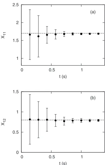
To illustrate this point, we calculate the eigenvalues of ⌶ˆ−1 _{under various assumptions about the number of known} parameters in the model. The results of this analysis are shown in Fig.6. It can be seen from the figure that when no information is available about model parameters共i.e., all the parameters are unknown兲, the largest eigenvalue of⌶ˆ−1_has an initial value of the order 102 and decays to 10−2 over a measurement timet= 1.3 s. The correlation between the de-cay of the largest eigenvalue and the convergence of the ␩ parameters in this case is evident from Fig. 5. When the coefficients of the cubic and quadratic terms in system 共4兲

are known, the value of the largest ␭iof ⌶ˆ−1共shown by the blue dashed line in Fig. 6兲 is reduced by three orders of

magnitude. When all parameters of the system共4兲are known except the control parameters ␩i, the largest value of ␭i of ⌶ˆ−1 _{共shown by the black dotted lines in Fig. 6兲 is further} reduced by two orders of magnitude.

In the latter case, convergence of the inferred parameters

␩ito their true values is much faster. To verify this point, the following test was performed: 共i兲first a signal of length 1 s was generated with stationary dynamics and used to infer all the model parameters; 共ii兲 next, the parameters ␩i were changed in a steplike manner; and 共iii兲 the convergence of the inferred parameters␩iwas analyzed as a function of the length of the step. The results are shown in Fig. 7. It is

0.2 0.4 0.6 0.8 1

0 0.5 1

η1

t (s) (a)

10-5

100

105

0 0.5 1 1.5

<

λ

>

t (s)

0 0.2 0.4 0.6 0.8 1

0 0.5 1

η2

t (s) (b)

10-5

100

105

0 0.5 1 1.5

<

λ

>

[image:6.609.61.283.66.400.2]

t (s)

FIG. 5. 共a兲 and 共b兲 Convergence of the control parameters ␩1

[image:6.609.311.560.127.310.2]

and␩₂as functions of the measurement timet. Values of the model parameters for this numerical test are given in Table I. We have used nine data blocks with 5000 points in each block. The standard deviations of the inferred parameters shown by the vertical bars are calculated over 1000 realizations. The horizontal lines show the true values of the control parameters. The sampling rate was 35 kHz. The insets in both figures show the decay of the largest eigenvalue of⌶ˆ−1_.

TABLE III. Values of some of the original coefficients inferred using 30 000 points obtained from measurement matrix and real parameter reconstruction. The actual values 共second column兲 are compared with the inferred values共third column兲; relative errors are given as percentages in the last column.

Parameter Real Inferred Rel. error

X11 1.7 1.686459 0.796526

X₁₂ 0.8 0.794263 0.717092

X21 0.2 0.196746 1.626811

X₂₂ 0.9 0.898222 0.197610

␩1 0.4 0.406227 1.556788

␩2 0.3 0.302462 0.820660

␣1 −0.35 −0.351992 0.569082

␣2 −0.2 −0.200376 0.188228

b₁ 1.35 1.357427 0.550145

b2 1.2 1.203863 0.321885

c₁ −1.0 −0.999520 0.047957

c2 −1.0 −0.999114 0.088582

10-6

10-4

10-2

100

0.1 0.5 0.9 1.3

<

λi

>

t (s)

FIG. 6. 共Color online兲The largest eigenvalues␭iof the matrix ⌶ˆ−1_{under different assumptions: 共i兲when none of the coefficients}

[image:6.609.326.545.476.626.2]

evident that the time scale for the convergence of ␩ is ⬃20 ms as compared to the convergence over⬃1 s in Fig.

6. It is therefore clear that the computational delay time of ⬍500 ms desired for physiological applications can be achieved easily within our Bayesian framework. Next, we consider the efficiency of the method under nonstationary conditions.

IV. NONSTATIONARY DYNAMICS

We consider the situation when all parameters except ␩i 关Eq. 共4兲兴 are fixed at the values given in Table I, but the control parameters␩iare allowed to change, either stepwise or continuously.

A. Stepwise changes of control parameters

1. Unknown parameters

In this section, it is assumed that none of the parameters of the model are known and that they have to be inferred at each step of the measurements. The parameters␩1and␩2are allowed to change at random in time in a steplike manner, and remain constant between steps. The time interval

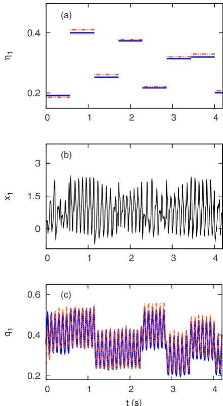
be-tween steps is approximately five periods of firing of the action potential and contains one block of data with 20 000 points. Other parameters of the model are fixed at the con-stant values given in Table I. At each step, we infer all pa-rameters of the model assuming their initial values to be zero and their initial dispersion to be infinity, as already discussed above.

The results of this test are shown in Fig.8. The inferred values of parameter␩1are compared with their true values in Fig.8共a兲. The time trace of the unknown coordinateq1共t兲 is compared with the corresponding reconstructed time trace q

˜₁共t兲in Fig.8共c兲. The latter time traces were reconstructed as

follows. First, the initial coordinates qi共t= 0兲 and variables

0 0.2 0.4 0.6 0.8

0 15 30 45 60

η1

t (ms)

(a)

-0.2 0 0.2 0.4 0.6 0.8

0 15 30 45 60

η2

t (ms)

[image:7.609.324.544.66.466.2]

(b)

FIG. 7. Typical example of the fast convergence of the control parameters共a兲␩1and共b兲␩2, as functions of time共length of signal兲.

The first point corresponds to 200 data points in one block. For each next point, the number of data points was increased by 200. The vertical lines show the standard deviations of the inferred values of the control parameters calculated over 1000 runs. The horizontal dashed lines indicate the true values of the parameters. The mixing matrix is defined in TableIII. The inferred parameters␩istart from an initial value of ␩₁=␩₂= 0.2 and converge quickly to the true values of ␩1= 0.4, ␩2= 0.3. The coefficients␣i, ␤i, ␥i, anddij are given in TableI. The noise amplitude is

冑

d₁=

冑

d₂= 0.012 25.

0.2 0.4

0 1 2 3 4

η1

(a)

0 1.5 3

0 1 2 3 4

x1

(b)

0.2 0.4 0.6

0 1 2 3 4

q1

[image:7.609.79.263.67.340.2]

t (s) (c)

FIG. 8. 共Color online兲 Inference of the parameters of two un-coupled FHN systems mixed by the measurement matrix. It is as-sumed that␩₁and␩₂change stepwise while all other parameters of the system are fixed and unknown. 共a兲 The inferred values of␩1 共dashed red lines兲 are compared with their true values 共full blue lines兲. 共b兲 Measured mixed values of the coordinate x1共t兲.共c兲 In-ferred values of the coordinateq1共t兲 共red dotted line兲are compared with its true values共blue solid line兲. The other parameters are fixed at the values given in Table I. The noise amplitude is

冑

d₁=

冑

d₂

vi共t兲were reconstructed using the inferred measurement ma-trix Xand Eqs. 共3兲and共10兲. Second, the variableq˜共t兲 was reconstructed using Eq. 共33兲of关6兴,

qi共t= 0兲=Xij −1

q ˜j共t= 0兲,

yi共t兲=Xij −1

yj共t兲,

q

˜共tk兲=␥h

兺

r=0 k

e−␤共tk−tr兲_y共_tr兲_+e−␤tk_q共0兲

−h␥

2 关y共tk兲+e −␤t_k

y共t0兲兴. 共17兲

It can be seen from the figure that the time resolution of the method is of the order of 500 ms even in the case when none of the model parameters is known. As mentioned above, however, the time resolution of the method can be improved substantially by considering the other parameter of the model to be known on the time scale of a few seconds

共corresponding to their correlation time, see Sec. II兲 and

tracking in time only the time-varying control parameters␩i.

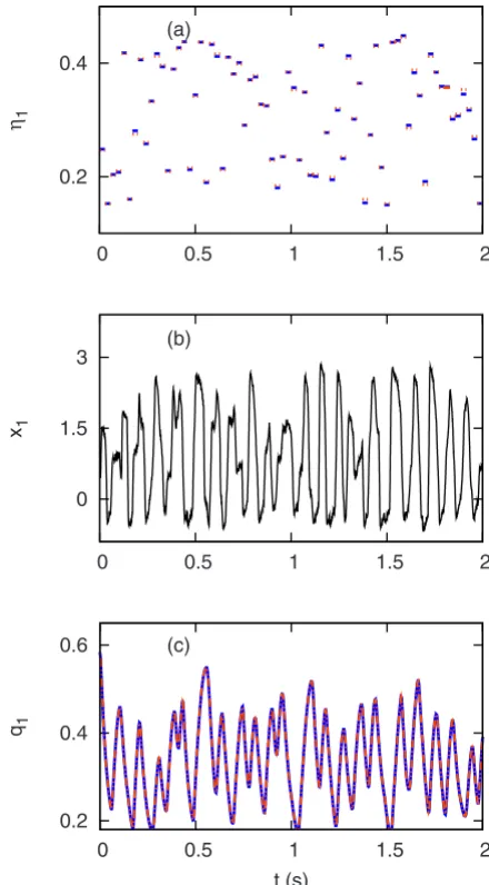
2. Tracking control parameters with known dynamics

We now investigate how fast physiological parameters can be tracked in time. It was shown above共see Sec. III C兲 that the convergence speed depends on information about the model parameters that is availablea priori, and that the fast-est time resolution can be achieved when all the parameters of the model, except the control parameters ␩i, are known. To demonstrate this effect, we now assume that ␩₁ and ␩₂ change stepwise at random and remain constant between steps as above, but that all other parameters of the model remain fixed at known values. The time interval between steps is now approximately 0.03 s and contains one block of data with 1000 points. The results of Fig. 9 show that the method can track random, stepwise variations of the control parameters with a time resolution of less than 0.03 s 共i.e., smaller by more than two orders of magnitude than in the previous case where all parameters had to be inferred兲.

B. Continuously varying control parameters with noise

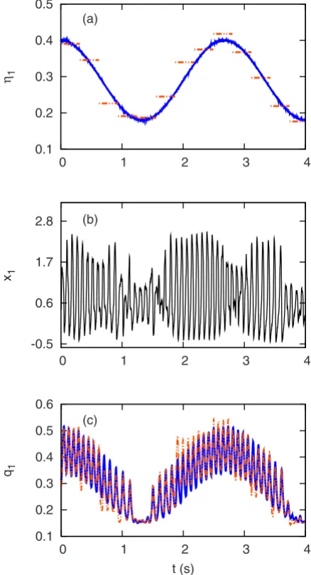
To complete our analysis of the reconstruction of nonsta-tionary dynamics of the physiological model, we now infer smoothly varying parameters ␩₁ and ␩₂ with added noise, without knowing any other parameters of the model. The test is performed as follows:共i兲 all parameters of the model are inferred from the first block共with 30 000 points兲of station-ary dynamics; 共ii兲 for all other blocks of data, we use ac-quired information to fix the model parameters constant at the inferred values, and track in time only variations of the control parameters ␩i. Each block of data 共except the first one兲contains 12 000 points and has a time lengtht⬇0.34 s. The time traces of the unknown variables qi共t兲 are recon-structed at every step using Eqs. 共17兲 as explained above. The inferred time evolution of the control parameters ␩i is compared with its true variation in Fig.10. It is evident from the figure that the method allows us to infer the unknown

constant parameters of the model, and then also to use this information to track in time the nonstationary control param-eters of the system with a time resolution of the order of 0.3 s.

V. CONCLUSION

In summary, we have explored the performance of the Bayesian inferential framework for nonstationary dynamics that we introduced in paper I 关6兴in relation to physiological applications. We did so by modeling a physiological signal as a set of fast variablesyi, mixed by an unknown

measure-0.2 0.4

0 0.5 1 1.5 2

η1

(a)

0 1.5 3

0 0.5 1 1.5 2

x1

(b)

0.2 0.4 0.6

0 0.5 1 1.5 2

q1

[image:8.609.324.544.66.464.2]

t (s) (c)

FIG. 9. 共Color online兲Inference of the model parameters of two uncoupled FHN systems mixed by the measurement matrix. It is assumed that␩1and␩2change stepwise while all other parameters

of the system are fixed and known. 共a兲 Inferred values ␩1 共short

elements of red dashed line兲 are compared with their true values

共short elements of full blue line兲as a function of time.共b兲The time trace of the measured coordinate x1共t兲. 共c兲 The time trace of the inferred coordinate˜q1共t兲 共red dotted line兲is compared with its true valueq1共t兲 共blue solid line兲. The values of the other parameters are fixed, as given in Table I. The noise amplitude is

冑

d1=

冑

d2

ment matrix, corresponding to the action potentials of sto-chastic FHN oscillators. Our goal was to see whether we could track on-line the control parameters ␩i of the model, given that these can vary with correlation time ␶cor ⱗ500 ms. It was assumed that the slow recovery variables of the FHN oscillators were unavailable for measurement and that the correlation time of all other unknown parameters of the model was of the order of 5 s. We have established that the method does indeed facilitate on-line tracking of␩iwith a time resolution ⬍0.3 s. This was achieved by embedding

the fast on-line tracking of the control parameters within a Bayesian learning framework for the more slowly varying parameters of the system with a time resolution⬍1 s.

We showed that the time resolution of the method is de-termined by the eigenvalues of the matrix⌶ˆ−1_=Dˆ_丢⌽ˆ

k −1_{, and} therefore depends essentially on the choice and scale of the base functions. Note that, while the eigenvalues of Dˆ are intrinsic to the system, the choice and scale of the base func-tions can be controlled by the researcher. Specifically, we demonstrated that by accumulating a priori information about slowly varying model parameters, one can enhance the time resolution of the control parameters by an order of mag-nitude.

Several limitations of the method should be borne in mind in adapting it to any particular application. As we have al-ready mentioned, fast online applications require that mea-surement noise be small. In addition, it was assumed that the equations for the hidden variables are linear and determinis-tic. The latter limitations can be removed, at least partially, by writing the equation for the hidden variables in the more general form q˙=f共q兲+g共y兲, where the homogeneous equa-tion q˙=f共q兲 is integrable and the nonlinear function of the measurable variableg共y兲 is arbitrary. One can then proceed in exactly the same way as described in the present paper. Furthermore, the method can be extended to encompass the case of an integrable stochastic differential equation for the hidden variables. To do so, a stochastic integral must be added to the right-hand sides of the equations of reduced dynamics. Finally, the method can be applied to the case in which the dynamics of the system jumps at random between different states, as, for example, in gating dynamics. Note, however, that if the different states are characterized by dif-ferent dynamical models, then the solution of the inference problem can be obtained more generally within the frame-work of a hybrid probabilistic approach, as will be described in more detail elsewhere. We note that the method is also useful when the low-dimensional dynamics is only a rough approximation to the actual multidimensional complex dy-namics of the system. The latter situation is often the case in physiological and aerospace applications关21,22兴.

We conclude, therefore 共see also关6兴兲, that the results

ob-tained are of broad interdisciplinary interest. They were re-cently shown to be particularly useful in medical applica-tions 关20兴 and for the development of prognostics and diagnostics techniques in aerospace applications关21,22兴. The

method can readily be extended to encompass systems with multiplicative and colored noise, and efforts toward these ends are already in progress.

ACKNOWLEDGMENTS

We are grateful to the Engineering and Physical Sciences Research Council共UK兲and NASA for financial support, and to A. Stefanovska for valuable discussions.

0.1 0.2 0.3 0.4 0.5

0 1 2 3 4

η1

(a)

-0.5 0.6 1.7 2.8

0 1 2 3 4

x1

(b)

0.1 0.2 0.3 0.4 0.5 0.6

0 1 2 3 4

q1

[image:9.609.62.281.70.474.2]

t (s) (c)

FIG. 10. 共Color online兲Inference of␩₁and␩₂while smoothly varying in the presence of noise. No prior knowledge of the model parameters is assumed.共a兲The inferred values of ␩₁共dashed red lines兲are compared with their true values共full blue lines兲.共b兲The measured time trace of the mixed coordinatex1共t兲.共c兲The inferred time trace of the mixed coordinate˜q1共t兲 共dashed red line兲is com-pared with its true value q1共t兲 共full blue line兲. The values of the other parameters are given in Table I. The noise amplitude is

冑

d₁

关1兴R. Mukkamala and R. J. Cohen, Am. J. Physiol. Heart Circ. Physiol. 281, H2714共2001兲.

关2兴S. Lu and K. H. Chon, IEEE Trans. Signal Process. 51, 3020

共2003兲.

关3兴A. B. Schwartz, X. T. Cui, D. J. Weber, and D. W. Moran, Neuron 52, 205共2006兲.

关4兴F. Lotteet al., J. Neural Eng. 4, R1共2007兲.

关5兴S. Eyal and S. Akselrod, Methods Inf. Med. 39, 118共2000兲.

关6兴D. G. Luchinsky, V. N. Smelyanskiy, A. Duggento, and P. V. E. McClintock, preceding paper, Phys. Rev. E 77, 061105共2008兲.

关7兴R. FitzHugh, Biophys. J. 1, 445共1961兲.

关8兴J. Nagumo, S. Animoto, and S. Yoshizawa, Proc. IRE 50, 2061

共1962兲.

关9兴A. T. Winfree, The Geometry of Biological Time 共 Springer-Verlag, New York, 1980兲.

关10兴J. Keener and J. Sneyd, Mathematical Physiology共 Springer-Verlag, New York, 1998兲.

关11兴E. N. Best, Biophys. J. 27, 87共1979兲.

关12兴J. Rogers and A. McCulloch, IEEE Trans. Biomed. Eng. 41, 743共1994兲.

关13兴R. R. Aliev and A. V. Panfilov, J. Theor. Biol. 81, 33共1996兲.

关14兴P. Chen, SIAM J. Math. Anal. 23, 81共1992兲.

关15兴O. Berenfeld and S. Abboud, Med. Eng. Phys. 18, 615共1996兲.

关16兴D. Bullock, P. Cisek, and S. Grossberg, Cereb. Cortex 8, 48

共1998兲.

关17兴S. Rajasekar and M. Lakshmanan, J. Theor. Biol. 166, 275

共1994兲.

关18兴R. Mannella, Int. J. Mod. Phys. C 13, 1177共2002兲.

关19兴D. M. Bates and D. G. Watts, Nonlinear Regression and Its Applications共Wiley, New York, 1988兲.

关20兴D. G. Luchinsky, M. M. Millonas, V. N. Smelyanskiy, A. Per-shakova, A. Stefanovska, and P. V. E. Mcclintock Phys. Rev. E

72, 021905共2005兲.

关21兴V. V. Osipov, D. G. Luchinsky, V. N. Smelyanskiy, and D. A. Timucin, Proceedings of the AIAA/ASME/SAE/ASEE Joint Propulsion Conference and Exhibit, AIAA Conference Pro-ceedings共AIAA, Cincinnati, OH, 2007兲, AIAA 2007-5823.