Volume 12, Number 9, 2005 © Mary Ann Liebert, Inc. Pp. 1183–1201
Algorithms for Selecting Informative Marker Panels
for Population Assignment
NOAH A. ROSENBERG
ABSTRACT
Given a set of potential source populations, genotypes of an individual of unknown origin at
a collection of markers can be used to predict the correct source population of the individual.
For improved efficiency, informative markers can be chosen from a larger set of markers to
maximize the accuracy of this prediction. However, selecting the loci that are individually
most informative does not necessarily produce the optimal panel. Here, using genotypes from
eight species—carp, cat, chicken, dog, fly, grayling, human, and maize—this univariate
ac-cumulation procedure is compared to new multivariate “greedy” and “maximin” algorithms
for choosing marker panels. The procedures generally suggest similar panels, although the
greedy method often recommends inclusion of loci that are not chosen by the other
algo-rithms. In seven of the eight species, when applied to five or more markers, all methods
achieve at least 94% assignment accuracy on simulated individuals, with one species—dog—
producing this level of accuracy with only three markers, and the eighth species—human—
requiring
∼
13–16 markers. The new algorithms produce substantial improvements over use
of randomly selected markers; where differences among the methods are noticeable, the
greedy algorithm leads to slightly higher probabilities of correct assignment. Although none
of the approaches necessarily chooses the panel with optimal performance, the algorithms
all likely select panels with performance near enough to the maximum that they all are
suitable for practical use.
Key words: ancestry inference, informativeness, microsatellites, population structure.
1. INTRODUCTION
S
ituations often arise in which the source populationor populations for genetic material from individuals of unknown origin must be determined (Anderson and Thompson, 2002; Davies et al., 1999; Guinand et al., 2002; Hansen et al., 2001; Lowe et al., 2001; Manel et al., 2005; Waser and Strobeck, 1998; Ziv and Burchard, 2003). In a typical scenario, allele frequencies at a set of loci are given for several predefined groups, and using their genotypes at these loci, unknown individuals are each assigned to a single source population (Banks and Eichert, 2000; Baudouin et al., 2004; Buchanan et al., 1994; Paetkau et al., 1995; Primmer et al., 2000; Pritchard et al., 2000; Rosenberg et al., 2003).Department of Human Genetics, Bioinformatics Program, and the Life Sciences Institute, University of Michigan, Ann Arbor, MI.
In an increasing number of species, the number of markers for which allele frequencies are available exceeds that required for accurate assignments. Thus, to perform assignment procedures efficiently, the panel of loci for genotyping of unknowns can be chosen from a larger collection of markers to contain as much information about ancestry as possible. Two of the questions that arise in the selection of an efficient panel are:
1. Given a collection of L loci and a desired number of markers M < L to genotype, which markers
should constitute a panel of sizeM?
2. How should the number of markers to genotype,M, be determined?
To answer question 2, for each number of markers from 1 to L, a measure of the “performance” of
marker panels (either random panels or those selected using answers to question 1 can be evaluated, andM
can be chosen as the smallest number for which the performance exceeds a specified threshold (Bamshad et al., 2003; Banks et al., 2003; Bernatchez and Duchesne, 2000; Campbell et al., 2003; Cornuet et al., 1999; Edwards, 2003; Manel et al., 2002; Risch et al., 2002; Rosenberg et al., 2001, 2003; Turakulov and Easteal, 2003). In this analysis, one of several possible procedures for measuring performance can be used. Question 1 poses greater difficulties. A simple answer suggests evaluation of an information-content
statistic for each marker, followed by assembly of a panel consisting of theMmost “informative” markers,
or of any M markers individually more informative than a specified threshold (Collins-Schramm et al.,
2002; Dean et al., 1994; Manel et al., 2002; Rosenberg et al., 2001, 2003; Shriver et al., 1997). These approaches produce higher performance than use of random markers (Rosenberg et al., 2001, 2003). However, they need not lead to the set with maximal performance (Pfaff et al., 2004; Rosenberg et al., 2003): in Fig. 1, Locus 1 is most informative, but the most informative pair of loci is {Locus 2, Locus 3}. In fact, in Fig. 1, the two loci that are most informative individually comprise the least informative pair.
The explanation for why selecting markers that are most informative individually need not lead to an optimal panel lies in the fact that the ability of a marker to assign an individual correctly depends on the source population of the individual. A panel of markers that are generally useful for all source populations
may be less efficient than a panel of markers that are generally poor but in which for eachm, the mth
marker is extremely informative for themth source population. ConsiderK≥3 populations and a setX
[image:2.612.88.487.444.653.2]ofKloci, numbered 1 throughK, in which each locus hasKalleles. For locusm∈X, themth allele has
frequency 1 in themth population and frequency 0 in all other populations; all other alleles of locusm
have frequency 1/(K−1) in all except the mth population. Using the fORCA measure of performance
(Section 2.2), which gives the probability of correct assignment if multilocus genotypes are assigned to the population from which they are most likely to have originated, for one of these loci, the probability that an
individual is assigned to the correct source population is 2/K. However, using allK loci, this probability
is 1, because every possible multilocus genotype for theK loci is observed in only one population.
Now consider a second set Y of K loci, each of which also has K alleles. For each locus in Y, the
mth allele has frequency 1−(K −1)ε in themth population and frequency ε in all other populations,
where 0 < ε < (K −2)/[K(K −1)]. Using fORCA, the probability of correct assignment for such a
locus is 1−(K−1)ε, which is larger than 2/K. Thus, any locus inY gives a higher correct assignment
probability than any locus in X. However, because every genotype is found in every population, no
multilocus genotype at the loci in Y can be assigned with certainty to a particular source population.
Consequently, the probability of correct assignment for the setY is less than 1, and the panel of generally
informative markers is less useful than the panel of markers that are each informative for only one source population.
To account for the fact that the performance of a set of markers need not be expressible solely in terms of performances of individual markers, I consider multivariate algorithms for selecting efficient panels of size
M from amongL loci. In analytical and simulation-based forms, these algorithms, as well as sequential
accumulation of individually informative markers, are applied to data from various species. Using simulated individuals, the performances of the algorithms in population assignment are then compared.
2. ALGORITHMS FOR SELECTING MARKER PANELS
2.1. Algorithms based on a given “performance function”
For a finite set SLcontainingLloci, denote the set of all its subsets byP(SL). Letφdenote the empty
set.
Definition. Consider a function f : P(SL) → R. Function f is a performance function for SL if f (T1)≤f (T2)for any finiteT1, T2⊂SLwithT1⊂T2.
Informally, a performance function measures “performance” of a collection of markers in population assignment; higher values indicate better performance, so that subsets of a set of markers have equal or poorer performance than the set itself. Specific examples are discussed in Section 2.2; we will see later that
iff is the function that measures the probability of correctly assigning individuals when each multilocus
genotype for a set of loci is assigned to the population in which it is most likely to occur, thenf is a
performance function.
Question 1 from Section 1 can now be rephrased: given a set SL ofL loci, a performance function f
and a positive integer M < L, identify the subset of SL that maximizes f over all subsets of SL with
cardinalityM. Several methods can be used to choose a setSM to serve as a candidate for this optimal set.
In each of the following approaches, ties for the choice of set are broken randomly. The first method is
to evaluatef for all possible candidate sets.
Method 1 (exhaustive evaluation). ForM≥1, define
SM =arg max
T∈P(SL)
|T|=M
f (T ).
Two computational difficulties arise in application of Method 1. First, for sufficiently largeM, evaluation
of f (T ) may be impractical when |T| = M. Second, for sufficiently large L and M, even if it were
possible to evaluatef (T )when |T| =M, the number LCM of subsets ofSL with cardinalityM is very
large and the subsets cannot be exhaustively tested.
If L or M is large enough that Method 1 is not feasible, an algorithm that is less computationally
follow each sequentially accumulate loci to marker panels. Thus, Methods 2–4 are all greedy algorithms,
in that each constructsSM from SM−1 together with the “best” remaining locus by some criterion. For
convenience, however, Methods 2, 3, and 4 are labeled “univariate,” “greedy,” and “maximin,” respectively. The simplest of the three computationally feasible algorithms is the procedure discussed in Section 1,
which proposes evaluation of loci individually, and which definesSM as the set containing theMloci that
have the highest individual values.
Method 2 (univariate accumulation). DefineS0=φ, and forM≥1, define
SM =SM−1∪
arg max
v∈SL\SM−1 f ({v})
.
This algorithm is convenient, but as discussed in Section 1, iff depends on interactions among contributions
of individual markers, the procedure might fail to choose the set with maximal performance.
To incorporate multivariate dependence of f while reducing the computational burden of Method 1, a
procedure can be used that chooses the next marker in the panel conditional on the information obtained from those markers that have already been included.
Method 3 (greedy accumulation). DefineS0=φ, and forM≥1, define
SM =SM−1∪
arg max
v∈SL\SM−1
f ({v} ∪SM−1)
.
To choose theMth marker, this algorithm evaluates each of the remaining markers together with theM−1
markers that have already been chosen and selects the marker that gives the highest value off. Method 3
is more computationally feasible than Method 1 in that for eachM, only L−M+1 rather than LCM
sets must be tested. However, like Method 1, Method 3 is not practical ifM is sufficiently large. This
procedure is also not guaranteed to locate the set with maximal performance (Fig. 1).
The final algorithm takes into account multivariate dependence and has greater computational feasibility than Methods 1 and 3, but also does not necessarily maximize performance.
Method 4 (maximin accumulation). Chooser≥2 small enough that for M≤r,SM is obtained by Method 1. ForM > r, define
SM =SM−1∪
⎧ ⎨
⎩argv∈SmaxL\SM−1
min
T∈P(SM−1)
|T|=r−1
f ({v} ∪T )
⎫⎬ ⎭
Note that this algorithm has two parts: for smallM, exhaustive evaluation is performed. For larger M,
the method accumulates loci that contribute new information, conditional on the information from markers
that have already been selected: it chooses theMth marker from among the remaining markers as the one
with the maximal value of the minimumf, where the minimum is taken across all sets in which the other
M−1 markers are among those that have already been selected.
Other “hybrid” algorithms are possible. In increasing order of ability to locate the set with maximal performance, but also in increasing order of difficulty of computation, the methods are ordered 2, 4, 3, 1.
Thus, for a given set of loci, asM is increased, Method 1 can be used until LCM becomes too large
for exhaustive evaluation of all subsets of cardinalityM. Method 3 can then be used to add new loci to
the existing set untilM becomes too large for evaluation of any sets with cardinalityM. Method 4 can
then be used untilLCr is too large for evaluation of all subsets of cardinalityr, reducingr to 2 as the
computational burden increases. Finally, if no other options are available, Method 2 is likely to be feasible
in any realistic scenario. The specific choice of the performance functionf affects the values ofLandM
2.2. Performance functions
To evaluate the potential of a set of loci to provide information about ancestry, I consider an analytical approach and a closely related simulation approach. The simulation procedure and modifications of it are frequently used to assess performance of sets of loci (Banks and Eichert, 2000; Banks et al., 2003; Buchanan et al., 1994; Campbell et al., 2003; Paetkau et al., 1995, 2004; Waser and Strobeck, 1998); the analytical approach uses the formula that underlies the simulation procedure (Rosenberg et al., 2003).
Consider a set SM containing loci m=1,2, . . . , M, with locus mhaving alleles j =1,2, . . . , N(m).
Consider populationsi =1,2, . . . , K, with the relative frequency of allelej of locusmin population i
equalingp(m)ij . Suppose that at each locus, in each population, the two alleles of a diploid individual are
independent: that is, for each i, j, h, and m, an individual in populationi has genotypejh at locus m
with probability(2−δjh)p(m)ij pih(m), where jh is the same genotype as hj andδjh is 1 if j =h and 0
otherwise. Suppose also that within each population, genotypes are independent across loci, and that for
each i, individuals of unknown origin have prior probability 1/K of having derived from population i.
If we consider decision rules where each possible multilocus diploid genotype has a specified probability of being assigned to each of the potential source populations, the rule that produces the optimal rate of correct assignment (ORCA) simply assigns an individual to the population from which its genotype is most likely to have originated (Rosenberg et al., 2003). The probability that an individual is assigned to its correct population of origin is
fORCA(SM)=
N(1)
j(1)
1 =1
N(1)
j(1)
2 =j(
1)
1 N(2)
j(2)
1 =1
N(2)
j(2)
2 =j(
2)
1 · · · N
(M)
j1(M)=1 N(M)
j2(M)=j1(M)
max i∈{1,2,...,K}
1 K
M
m=1
(2−δj(m)
1 j2(m))p
(m) ij1(m)
p(m)
ij2(m)
.
(1)
For the empty set, fORCA(φ) = 1/K. It can be shown that fORCA is indeed a performance function
(Theorem 2 in the appendix).
Conveniently, because of its relationship to assignment by most likely source population, fORCA(SM)
can be approximated using the following simulation.
1. From a uniform prior on{1,2, . . . , K}, simulate the source population, q, of an individual.
2. Independently for each locusm∈SM, simulate two independent alleles,j1(m) andj2(m), from the allele
frequency distribution of population q.
3. Compute
γ =arg max
i∈{1,2,...,K}
1 K
M
m=1
(2−δj(m)
1 j2(m))p
(m) ij1(m)
pij(m)(m)
2
.
In case of a tie in the value of the product for two or more values ofi, randomly assign one of thesei
to equalγ. Ifγ =q, the individual is assigned correctly.
4. Repeat steps 1–3 many times, computing the fraction of simulated individuals that are correctly assigned.
The result is f˜ORCA(SM).
For the empty set, f˜ORCA(φ) = 1/K. An advantage of evaluating the less precise f˜ORCA rather than
fORCA is that the simulation can be performed quickly for large values ofM, whereas if the number of
terms summed in Equation (1), orMm=1(N(m)+1)N(m)/2, is large, then Equation (1) cannot realistically
be evaluated. In a strict sense,f˜ORCA is only approximately a performance function (Corollary 6 in the
appendix), as stochasticity makes it possible for a set of loci to have a lower value off˜ORCAthan one of its
proper subsets; however, because of its close relationship tofORCA,f˜ORCAis treated here as a performance
3. DATA
Methods 2–4 and fORCA and f˜ORCA are applied to selection of marker panels using data from eight
species (Table 1). The datasets each consist of unphased individual multilocus diploid genotypes for autosomal microsatellite loci (Goldstein and Schlötterer, 1999) spread throughout the genomes of their respective species. They span a wide range in number of markers and populations, as well as in levels of genetic diversity within populations and of genetic divergence across populations.
4. IMPLEMENTATION
4.1. Computation of
fORCA
and
fORCA
˜
Allele frequencies at a locus were estimated from the data using the ratios of the numbers of ob-served copies of alleles to the total number of observations for the locus. In each dataset, for each locus and population, individuals were assumed to have two independent alleles. This assumption of Hardy– Weinberg proportions holds for most locus-population pairs, although the fraction of pairs at which it is violated is large in some populations (Irion et al. [2003] for example). A substitute for this assumption is
replacement of the product of allele frequencies,(2−δj(m)
1 j2(m))p
(m) ij1(m)
p(m)
ij2(m)
, in Equation 1 and in Step 3
of the simulation procedure, with the genotype frequencyp(m)
i(j1(m)j (m)
2 )
, and simulation from the genotype
frequency distribution in Step 2 rather than from the allele frequency distribution. However, the large number of possible genotypes compared to typical per-population sample sizes makes it more difficult to obtain accurate estimates of genotype frequencies than of allele frequencies. When sample sizes are too small for this approach to be feasible, genotype frequencies estimated from allele frequencies and a single parameter measuring the deviation from Hardy–Weinberg proportions—the inbreeding coefficient (Ayres and Balding, 1998)—could potentially be used. For simplicity, however, Hardy–Weinberg propor-tions were assumed here. Additionally, because markers were generally widely spaced across the genomes of the various species, in each population, genotypes at different loci were assumed to be independent.
Because the allele frequencies were estimated from samples that were in general small compared to the numbers of alleles at loci, similarly to previous implementations (Banks and Eichert, 2000; Campbell et al., 2003; Paetkau et al., 2004; Waser and Strobeck, 1998), a slight alteration was made to the computation
off˜ORCA: 1/(Z+1)was substituted in place of allele frequencies of 0 in Step 3, whereZ is the largest
number of alleles genotyped at any locus in any population. This substitution reflects the fact that even if its sample frequency is 0, an allele may be present in a population at nonzero frequency. However, because the simulations were performed assuming that the sample frequencies equal the true allele frequencies
(Step 2), the use of 1/(Z+1)in place of a true frequency of 0 systematically decreasesf˜ORCAcompared
tofORCA; note that this change has little effect if most alleles are found in most populations, so that allele
frequencies of 0 are rare. The corresponding substitution of 0 with 1/(Z+1)was not made in computation
offORCA, as this substitution can only increase the value of fORCAand therefore is anticonservative.
4.2. Selection of marker panels
Because of the sizeable number of alleles at the microsatellite loci in the data, for sets of approximately
four or more loci, the number of possible multilocus genotypes was quite large and evaluation offORCA
forM ≥4 proceeded very slowly. Thus, in Method 4, r =2 was chosen, as the use of evenr =3 was
impractical for the datasets with the largest numbers of loci and alleles. In each of the datasets, the number
of loci was sufficiently small thatfORCAandf˜ORCAcould be evaluated relatively rapidly for allLC2pairs
of loci.
Of the eight possible combinations of methods (1, 2, 3, and 4) and functions (fORCA andf˜ORCA), five
were practical to implement on the datasets for all possible values ofMandL: panels were obtained using
bothfORCA andf˜ORCA with Methods 2 and 4 and usingf˜ORCA with Method 3. In case two or more loci
Table2. Robustness of Sets of Selected Markers that Were Obtained Using Simulations withf˜ORCAa
Kendall coefficient of Mean across loci of standard concordance of rankings deviation of rank across replicates
Method 2 Method 3 Method 4 Method 2 Method 3 Method 4 Species (univariate) (greedy) (maximin) (univariate) (greedy) (maximin)
Carp 0.977 0.740 0.972 0.39 1.46 0.49
Cat 0.923 0.808 0.910 0.66 1.18 0.70
Chicken 0.984 0.445 0.961 0.90 5.71 1.38
Dog 0.966 0.183 0.981 5.12 26.74 3.85
Fly 0.979 0.208 0.978 3.09 20.29 3.17
Grayling 0.976 0.622 0.973 0.55 2.31 0.63
Human 0.940 0.125 0.980 26.09 105.63 15.21
Maize 0.983 0.177 0.988 3.55 26.85 2.98
aFor Method 4, if the marker ranked 1 was not included in the top-ranked pair, the two loci in the top-ranked pair were assigned
rank 1.5 and the top-ranked marker was assigned rank based on the later stage at which it re-entered the list. This scenario was generally unusual, occurring for none of the 10 replicates in chicken, grayling, and maize, 1 of 10 in carp, cat, and dog, and 3 of 10 in fly, but 8 of 10 in human.
In application off˜ORCA, it is necessary to simulate enough individuals that robust rankings are obtained.
Thus, for each dataset, 10 replicates were performed for each of Methods 2, 3, and 4, using 1,000
individu-als to evaluatef˜ORCAfor each proposed panel. For each replicate, each locus was associated with a number
in{1,2, . . . , L}, indicating the step at which the locus was accumulated to the set of selected markers (for
example, in Fig. 1, using Method 3, Locus 1 is added at the first step, Locus 3 at the second step, and Locus 2 at the third step). The Kendall coefficient of concordance (Gibbons, 1985, p. 250) of the ten marker “rankings” obtained in this manner was then computed. Also, the mean across loci of the standard deviation of locus “ranks” across replicates was calculated. Except for those based on simulations with the greedy algorithm, rankings in independent replicates were highly concordant, and loci varied little in rank across replicates (Table 2). For the greedy algorithm, after enough markers for nearly perfect assignment have been accumulated, additional markers are selected essentially randomly, because none of the markers contribute to an increase in performance. Thus, less concordance of marker sets is to be expected if the number of markers is sufficient for highly accurate assignment. Even though the marker panels in replicate simulations differed in composition, however, these panels had very similar performance. For all datasets and each
pos-sible number of markersM, the values off˜ORCAfor the 10 panels suggested by the greedy algorithm were
nearly always within 0.04 of each other; only occasionally was the range of the 10 values larger than 0.01.
Thus, use of 1,000 simulated individuals to compute f˜ORCAwas assumed to be sufficient for selection
of marker panels; to be conservative, in all f˜ORCA computations other than those that underlie Table 2
(and those applied to random sets of markers—Section 4.3), 10,000 individuals were simulated. In larger datasets for which the simulation time with this number of individuals is prohibitive, fewer individuals could potentially be used, with a consequent decline in robustness of the rankings obtained.
In addition to the variability that results from the stochasticity of simulation, sampling provides a separate source of variability for rankings. However, in a previous analysis (Rosenberg et al., 2003), using
a performance function similar tofORCAwith datasets of comparable complexity to those in Table 1, values
of the performance function and the associated rankings based on Method 2 showed little variation across datasets in which bootstrap resamples of individuals were taken. Thus, although it might be nontrivial for the smallest of the datasets in Table 1, the impact of sampling variation on marker rankings was not investigated here.
4.3. Evaluation of performance
After marker panels were chosen using each of the five approaches, simulations were used to evaluate ˜
fORCAon the panels selected with Methods 2 and 4. For each set of loci, 10,000 individuals were simulated.
FIG. 2. Relationship of the difference between simulated and analytically obtained probabilities of correct assignment to the analytical probability. (A) Simulations performed with replacement of allele frequencies of 0 by 1/(Z+1). (B) Simulations performed retaining allele frequencies of 0. Both graphs were generated using the same simulated individuals. In (A), locus 3-4 in carp lies below the graph at (0.734,−0.151).
The performances of the five approaches were compared to those of random sets of markers. Each
marker was associated with a random number. For each number of lociM,f˜ORCA was evaluated (using
1,000 simulated individuals) for the set containing theM markers with the M highest random numbers.
This procedure was repeated for 100 random orderings of the markers.
5. RESULTS
As described in Section 2.2, f˜ORCA in principle estimates by simulation the same quantity computed
analytically byfORCA. Similar values of f˜ORCA andfORCA for individual markers were observed in all
data sets, withf˜ORCA< fORCA more often thanfORCA<f˜ORCA(Fig. 2A). The generally smaller values
off˜ORCAcompared tofORCAresult from the substitution of 1/(Z+1)for 0 in Step 3 of the computation
off˜ORCA. This interpretation is supported by the fact that when the substitution is not made, the simulated
and analytically obtained values are nearly equal (Fig. 2B). Note that for cat, in which most alleles have nonzero frequencies in both populations (Table 1), the substitution has little impact on the simulation.
Although f˜ORCA was sometimes ∼10% smaller than fORCA (Fig. 2A), when the same algorithm was
applied to selection of panels—Method 2 or 4—locus ranks when f˜ORCA was used as the performance
function were nearly identical to those obtained withfORCA (Tables 3 and 4). With the same algorithm
applied, correlation coefficients of marker rankings based on the analytically computed fORCA and the
simulatedf˜ORCAwere in most datasets larger than 0.99 (Table 3).
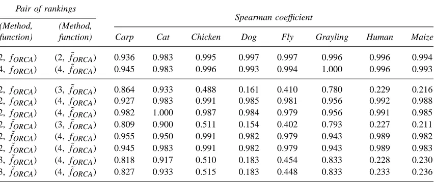
Table3. Spearman Coefficients of Rank Correlation between Pairs of Rankings of Markers
Pair of rankings
Spearman coefficient (Method, (Method,
function) function) Carp Cat Chicken Dog Fly Grayling Human Maize
(2,fORCA) (2,f˜ORCA) 0.936 0.983 0.995 0.997 0.997 0.996 0.996 0.994 (4,fORCA) (4,f˜ORCA) 0.945 0.983 0.996 0.993 0.994 1.000 0.996 0.993
[image:9.612.113.539.552.731.2]T able 4 . Ranks of Markers Selected Using Ea ch of Five Procedures a Locus rank (carp) Locus rank (cat) Locus f (2, f ) (2,
˜f)
(3,
˜f)
(4,
f
)
(4,
˜f)
Locus f (2, f ) (2,
˜f)
(3,
˜f)
(4,
f
)
(4,
˜f)
21-22 0.739 1 1 1 1 1 Fca96 0.831 1 1 1 1 1 3-4 0.734 2 4 2 3 3 Fca90 0.819 2 2 2 2 2 51-52 0.723 3 2 3 2 2 Fca23 0.812 3 3 3 3 3 85-86 0.671 4 3 5 5 4 Fca8 0.771 4 5 4 4 4 69-70 0.598 5 7 6 6 5 Fca45 0.763 5 4 6 6 5 111-112 0.588 6 6 9 7 6 Fca43 0.759 6 6 7 5 6 57-58 0.584 7 5 7 4 7 Fca77 0.680 7 7 5 7 7 29-30 0.511 8 8 4 8 8 Fca126 0.653 8 8 9 8 8 17-18 0.462 9 9 8 1 0 1 0 Fca35 0.578 9 9 8 9 9 55-56 0.387 10 10 11 9 9 89-90 0.337 11 11 10 11 11 Locus rank (c hic ken) Locus rank (do g) Locus f (2, f ) (2,
˜f)
(3,
˜f)
(4,
f
)
(4,
˜f)
Locus f (2, f ) (2,
˜f)
(3,
˜f)
(4,
f
)
(4,
˜f)
Locus rank ( fly) Locus rank (gr ayling) Locus f (2, f ) (2,
˜f)
(3,
˜f)
(4,
f
)
(4,
˜f)
Locus f (2, f ) (2,
˜f)
(3,
˜f)
(4,
f
)
(4,
˜f)
2189/2190 0.739 1 1 1 1 1 One2 0.728 1 1 1 1 1 2117/2118 0.708 2 2 6 3 3 BFR O13 0.594 2 2 2 2 2 1908/1909 0.701 3 5 5 7 5 BFR O18 0.509 3 3 4 3 3 2185/2186 0.700 4 3 3 4 4 BFR O12 0.500 4 4 8 6 6 2137/2138 0.680 5 4 2 2 2 Ogo2 0.500 5 5 5 5 5 2151/2152 0.679 6 9 22 8 9 BFR O10 0.453 6 6 7 8 8 1761/1762 0.676 7 6 10 6 6 BFR O11 0.438 7 7 3 4 4 2127/2128 0.664 8 7 27 9 8 BFR O15 0.428 8 9 13 7 7 2141/2142 0.660 9 8 15 15 15 BFR O5 0.424 9 8 10 10 10 2115/2116 0.659 10 12 19 11 10 MST73 0.374 10 10 6 9 9 2147/2148 0.655 11 14 25 10 12 MST85 0.242 13 13 9 1 3 1 3 2139/2140 0.652 12 10 4 5 7 2109/2110 0.597 22 25 9 1 4 1 4 2145/2146 0.568 31 30 7 2 3 2 1 1932/1933 0.566 32 32 8 2 4 2 3 Locus rank (human) Locus rank (maize) Locus f (2, f ) (2,
˜f)
(3,
˜f)
(4,
f
)
(4,
˜f)
Locus f (2, f ) (2,
˜f)
(3,
˜f)
(4,
f
)
(4,
˜f)
D21S2055 0.468 1 1 15 6 6 BNGL244 0.829 1 1 1 1 1 D2S1356 0.467 2 3 2 1.5 1.5 BNGL619 0.786 2 2 2 2 2 D22S683 0.463 3 2 12 5 5 MC1046 0.765 3 3 26 b 33 D1S1589 0.461 4 4 1 9 8 MC1191 0.738 4 4 5 4 5 D9S1871 0.456 5 6 3 4 4 MC1523 0.719 5 7 23 b 77 D8S560 0.452 6 5 5 1.5 1.5 MC1940 0.716 6 1 0 8 6 6 D14S1007 0.444 7 1 0 4 3 3 DUP28 0.711 7 9 53 b 81 3 D16S3401 0.441 8 8 116 b 11 10 MC1662 0.710 8 1 1 6 2 b 10 10 D7S2477 0.440 9 7 29 14 11 MC1890 0.702 9 1 3 7 5 1 1 F13A1-D6S 0.437 10 11 9 7 9 MC1194 0.701 10 5 4 6 b 99 D20S851 0.434 11 9 187 b 10 16 MC1371 0.694 11 8 1 2 1 2 8 D2S2986 0.423 15 15 6 1 7 1 4 BNGL105 0.687 12 12 4 1 5 4 D9S1779 0.409 19 23 7 8 7 MC1288 0.681 13 6 3 11 12 D11S2000 0.403 22 32 10 33 19 MC1740 0.658 17 16 6 1 3 1 4 D5S1501 0.402 24 28 8 4 0 2 4 MC1329 0.509 50 53 9 5 4 5 2 MC1931 0.455 66 63 10 55 54 aOnly those mark ers that appear among the 10 top-rank ed for one or more of the fiv e procedures are sho wn. F o r the maximin algorithms, the situation in whic h the top-rank ed pair of loci did not include the top-rank ed locus w as treated in the same w ay as in T able 2. Symbols f and
˜frefer
to
fORCA
and
˜fORCA
, respecti v ely . bIn the non-human datasets, these loci were added in the greedy algorithm at a stage when the pre vious combination of loci already produced perfect assi gnment (
˜fORCA
For pairs of rankings that used the same marker selection algorithm but different performance functions, correlation coefficients were generally larger than for pairs that used different marker selection algorithms and the same performance function (Table 3). However, Methods 2 and 4 produced highly correlated
rankings and lists with similar composition, regardless of whether fORCA or f˜ORCA was used as the
performance function (Tables 3 and 4). Note also that for chicken, a previous application of a univariate procedure based on a heterozygosity performance function (Rosenberg et al., 2001) produced the same
choice of the seven best-performing markers as Method 4 withfORCA.
Partly because of the fact that after enough markers for nearly perfect assignment have been selected, the greedy algorithm chooses new markers in an essentially random manner, lists of high-performing markers suggested by Method 3 were not very closely related to those obtained using the other algorithms (Tables 3 and 4). Especially for the larger datasets—dog, fly, human, and maize—the lists contained markers that were not included in panels suggested using the other algorithms. Simultaneously, many markers that were obtained using other algorithms did not appear among the lists suggested by the greedy method.
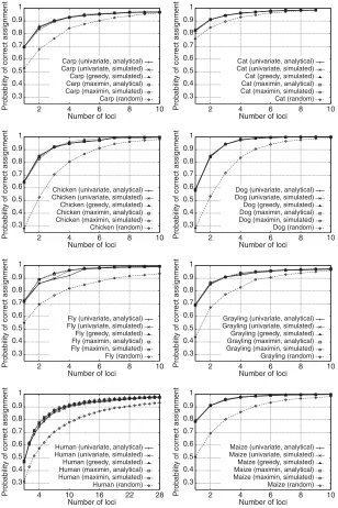
When f˜ORCA was evaluated for panels recommended by the selection algorithm/performance function
combinations, performance was substantially higher than that of random panels (Fig. 3). Other than in the human dataset, in which performance differed across combinations for many choices of the number of loci, all five combinations had nearly identical performance for most numbers of loci. In the human data, as the
number of loci ranged from 2 to 28, the greedy algorithm withf˜ORCAaveraged 0.013 higher performance
than the univariate algorithm withfORCA, and 0.015 higher than the univariate algorithm withf˜ORCA. Over
this range, the combinations involving the univariate algorithm were also slightly outperformed by those involving the maximin algorithm. When performance differences were noticeable in the other datasets—for example, in the situations when it exceeded 0.015 (carp with 2 loci, chicken with 2, 4, 5, and 6 loci, fly with 2, 3, and 4 loci, and grayling with 2 and 4 loci)—as was true in humans, the greedy algorithm
withf˜ORCA generally outperformed the other approaches. For each algorithm, performance function, and
dataset, performance appeared to converge as the number of loci increased.
6. DISCUSSION
Several combinations of marker selection algorithms and performance functions appropriate for choosing
a panel for use in ancestry inference have been suggested. As a consequence of the fact thatf˜ORCA has
expected value equal tofORCA(Rosenberg et al., 2003), the analytical and simulated performance functions
produced nearly identical panels. The panels obtained by straightforward selection of the most informative individual markers, although this procedure does not take into account interactions among markers, had nearly identical composition and performance to those obtained by the maximin procedure, which in the cases studied, makes use of bivariate interactions. The greedy procedure, although its recommended markers differed from those of the other procedures, generally did not produce substantially different performance.
The similarity in performance of the various procedures suggests that although counterexamples do exist, performance of a set of markers can almost be decomposed into univariate contributions of individual loci, with only a small contribution of bivariate and higher-order interactions. The greedy method is perhaps appropriate when slightly higher performance is desired. However, when simplicity, robustness, and ease of computation are needed, performance changes little when the univariate or maximin procedure is used in its place. Although none of the three algorithms—univariate, greedy, or maximin—is guaranteed to identify the panel of maximal performance, each likely selects panels that have performance sufficiently close to the optimum that any of the algorithms is suitable for use with data.
FIG. 3. Probability of correct assignment as a function of number of markers for five methods of selecting marker sets. The median probability of correct assignment based on 100 random orderings of the markers is also shown. For zero markers (not shown), the correct assignment probability is the reciprocal of the number of populations in the dataset. Note that the x-axis is scaled differently for the plots with the human dataset.
APPENDIX
It has sometimes been observed for certain ancestry inference procedures that accuracy of inference does not necessarily increase as markers are accumulated (Alaska Department of Fish and Game, 2000).
This appendix investigates the relationship offORCAandf˜ORCAto the number of loci, demonstrating that
fORCAdoes have the property that accumulating loci increases performance, and thatf˜ORCA“almost” has
this property. Thus, when evaluating the performance of f˜ORCA in assignment of individuals, although
Lemmas 1 and 3 give bounds for fORCA. Lemma 1 motivates the choice fORCA(φ) = 1/K, so that nonempty sets of loci produce correct assignment probabilities at least as large as those obtained with
no loci. Theorem 2 proves that fORCA is a performance function: if allele frequencies are known, the
probability of correct assignment for the procedure that assigns individuals to their most likely source
populations increases as additional loci are considered. Theorem 4 shows that the values offORCA for a
nested sequence of sets of loci converge to a constant, providing an explanation for the apparent convergence of performance in Fig. 3. This constant need not equal 1—for example, consider an infinite set of loci in
which for each locusl, each allele has frequency 1/N(l) in every population. For this set of loci, fORCA
equals 1/K.
Corollary 6 of Theorem 5 explains the assertion that f˜ORCA is “almost” a performance function. It
shows that if enough simulated individuals are used in the evaluation of f˜ORCA, with high probability,
accumulation of additional loci either increases performance, does not affect it, or decreases it by a small
amount. Corollary 8 of Theorem 7 gives a similar result in casefORCA is computed using sample allele
frequencies rather than true frequencies. If large enough samples are used in evaluation of this estimate, ˆ
fORCA, accumulating loci is likely to either increase performance, not affect it, or decrease it by a small
amount.
Finally, Corollary 10 of Theorem 9 shows that iff˜ˆORCA—performance based on simulations that employ
estimated allele frequencies—is used to evaluate assignments, then both the number of simulations and the sample sizes can be made large enough so that with high probability, accumulating additional loci either increases performance, does not affect it, or decreases it by a small amount. This result demonstrates that even under realistic conditions—in which simulations rather than the analytical formula are used and allele frequencies are estimated rather than known—the genotyping of additional loci is likely to increase the probability of correct assignment.
We now introduce additional notation before proving the theorems. Consider a vector Q of nonnegative
numbersq1, q2, . . . , qK with
K
i=1qi =1. The choice of Q corresponds to a prior probability distribution
for the source population of an individual; the purpose of introducing a general prior is to allow more general assignment rules. With the prior distribution Q, the probability of correct assignment if individuals
are assigned to their most likely source populations, denotedfQ, is obtained by replacing 1/K withqi in
Equation (1). The following form of this generalized quantity is more convenient for the proofs than is that of Equation (1) (though it is less convenient for evaluation due to its increased number of terms):
fQ(SM)=
N(1)
j(1)
1 =1
N(1)
j(1)
2 =1
N(2)
j(2)
1 =1
N(2)
j(2)
2 =1
· · · N(M)
j1(M)=1 N(M)
j2(M)=1 max i∈{1,2,...,K}
qi
M
m=1
pij(m)(m)
1
p(m)ij(m)
2
. (2)
The functionfORCA(Equation (1)) is the special case offQ in whichq1=q2=. . .=qK =1/K.
Definef˜Qby the simulation procedure in Section 2.2, replacing Step 1 with simulation ofqfrom the prior
Q. For a set of lociT, letf˜Q,α(T )be the (random) value off˜Q(T )obtained fromαsimulated individuals. Let fˆQ,(n1,n2,...,nK)(T ) be the (random) value of fQ(T ) obtained using allele frequency estimates from
a sample withni ≥1 observations in population i and abbreviate (n, n, . . . , n)by n. Let f˜ˆQ,α,n(T ) be
the (random) value off˜Q(T )obtained usingα simulated individuals based on allele frequency estimates
from a sample with size vector n. For the empty set, definef˜ˆQ,α,n(φ)= ˆfQ,n(φ)= ˜fQ,α(φ)=fQ(φ)=
maxi∈{1,2,...,K}qi.
Until now, we have viewed fORCA and its extensions as real-valued functions on sets of sets. For
a given set with M loci, it is convenient to also view them as functions on the set of possible allele
frequencies for the loci. In this framework, these functions have domainKN(1)×NK(2). . .×KN(M), where
N = {(p1, p2, . . . , pN|pj ≥ 0,
N
i=1pj = 1} is the set of possible allele frequencies for a single
population at a locus withN alleles. Henceforth, allele frequencies of 0 are retained in all computations.
Let WM = {(j1(1), j2(1), . . . , j1(M), j2(M))|j1(m), j2(m) ∈ {1,2, . . . , N(m)}for eachm}. Consider a
denu-merable set of lociSL, and without loss of generality, label the loci 1,2,3, . . . .LetRM denote the subset
ofSL that contains loci 1,2, . . . , M (R0 is the empty set). Note that in the main text,SL is assumed to
specifically assumes infinite SL. In case SL is finite, this result applies to infinite sets obtained by
ap-pending loci toSL so that for each positive integerl, at locusL+l, each allele has frequency 1/N(L+l)
in every population.
Lemma 1. For anyv∈SL,fQ({v})≥ max i∈{1,2,...,K}qi.
Proof. It suffices to show that for each Q, fQ(R1) ≥ max
i∈{1,2,...,K}qi. Using Equation (2), for any
k∈ {1,2, . . . , K},
fQ(R1)=
N(1)
j1=1
N(1)
j2=1
max i∈{1,2,...,K}
qip(1)
ij1pij2(1)
≥ N(1)
j1=1
N(1)
j2=1
qkp(1)
kj1pkj2(1).
Using the fact that for anym
N(m)
j1=1
N(m)
j2=1
p(m)kj1pkj2(m)=1, (3)
it follows thatfQ(R1)≥qk. Because this inequality holds for eachk,fQ(R1)≥ max
i∈{1,2,...,K}qi.
Theorem 2. FunctionfQ is a performance function forSL.
Proof. It suffices to show that for anyM ≥1, fQ(RM−1)≤fQ(RM). For M=1, the result follows
from Lemma 1. Otherwise, writing outfQ(RM−1)andfQ(RM)(Equation (2)), it suffices to show that for
any j∈WM−1,
max i∈{1,2,...,K}
qi M−1
m=1
p(m)ij(m)
1
pij(m)(m)
2
≤ N(M)
j1(M)=1 N(M)
j2(M)=1 max i∈{1,2,...,K}
qi M
m=1
p(m)ij(m)
1
pij(m)(m)
2
. (4)
For j ∈ WM−1, abbreviate ai = qi
M−1
m=1pij(m)(m) 1
p(m)
ij2(m)
. For j1(M), j2(M) ∈ {1,2, . . . , N(M)} and k ∈
{1,2, . . . , K},
akp(M)kj(M)
1
p(M)
kj2(M)
≤ max i∈{1,2,...,K}
aip(M)ij(M)
1
p(M)
ij2(M)
.
Summing this inequality over all possiblej1(M), j2(M)and using Equation (3), we obtain
ak≤
N(M)
j1(M)=1 N(M)
j2(M)=1 max i∈{1,2,...,K}
aip(M)ij(M)
1
p(M)
ij2(M)
.
Because this inequality holds for each k, we can take the maximum of the left hand side to obtain (4).
Lemma 3. For anyT ⊂SL,fQ(T )≤1.
Proof. By definition offQ, the result holds for the empty set. Otherwise, it suffices to show that the
result holds for everyRM,M≥1. ChooseM, and for eachk∈ {1,2, . . . , K}, let
WM,k =
j∈WM|arg max i∈{1,2,...,K}
qi
M
m=1
p(m)
ij1(m)
p(m)
ij2(m)
=k
For a given j, ifi1, i2, . . . , iC tie for the maximum, place j inWM,minc∈{1,2,...,C}ic. Rearranging Equation (2),
fQ(RM)=
K
i=1
qi
j∈WM,i M
m=1
p(m)
ij1(m)
p(m)
ij2(m)
≤ K
i=1
qi
j∈WM M
m=1
p(m)ij(m)
1
pij(m)(m)
2
=K i=1
qi
M
m=1
N(m)
j1(m)=1 N(m)
j2(m)=1
p(m)
ij1(m)
p(m)
ij2(m) .
Applying Equation (3), it follows thatfQ(RM)≤
K
i=1qi =1.
Theorem 4. Ifm1≤ m2 implies Tm1 ⊂Tm2 ⊂SL for allm1, m2, then {fQ(Tm)}∞m=1 converges to a
number in[maxi∈{1,2,...,K}qi,1].
Proof. As a consequence of Theorem 2, the sequence is monotonically nondecreasing. As a
conse-quence of Lemmas 1 and 3, it is bounded below by maxi∈{1,2,...,K}qi and above by 1. Using the fact that
monotonic bounded sequences of real numbers converge (Rudin, 1976, Theorem 3.14), the result follows.
Theorem 5. Consider T ⊂ SL. As α→ ∞,f˜Q,α(T )converges almost surely in and probability to ˜
fQ(T ).
Proof. The almost sure convergence is a consequence of the strong law of large numbers (Serfling,
1980, Theorem 1.8B), using the fact that for anyT,E[ ˜fQ,1(T )] =fQ(T )(see Section 2.2). Convergence
in probability then follows (Serfling, 1980, Theorem 1.3.1).
Corollary 6. ConsiderT ⊂SL, setsT1, T2 ⊂T with T1⊂T2, and1, 2>0. There exists α∗ such
that ifα≥α∗, thenP[ ˜fQ,α(T2) >f˜Q,α(T1)−1]>1−2.
Proof. Applying Theorem 5 and the definition of convergence in probability, there existsα∗ such that
forα≥α∗, bothP[| ˜fQ,α(T1)−fQ(T1)|< 1/2]>1−2/2 andP[| ˜fQ,α(T2)−fQ(T2)|< 1/2]>1−2/2.
Then P[ ˜fQ,α(T1) < fQ(T1)+1/2] > 1−2/2 and P[fQ(T2) < f˜Q,α(T2)+1/2] > 1−2/2, from
whichP[(f˜Q,α(T1) < fQ(T1)+1/2)∩(fQ(T2) < f˜Q,α(T2)+1/2)]>1−2. The intersection in this
expression has probability less than or equal to that off˜Q,α(T1)+fQ(T2) < fQ(T1)+ ˜fQ,α(T2)+1, which,
using Theorem 2 to obtain fQ(T1)≤ fQ(T2), has probability less than or equal to that of f˜Q,α(T2) >
˜
fQ,α(T1)−1.
Theorem 7. Consider T ⊂SL. Asn → ∞,fˆQ,n(T ) converges almost surely and in probability to ˆ
fQ(T ).
Proof. If T =φ the result is trivial. Otherwise, by the strong law of large numbers (Serfling, 1980,
Theorem 1.8B), for eachi,m, andj(m), asn→ ∞, the sample frequency pˆ(m)ij(m),n estimated from sample
size n converges almost surely to the true frequency p(m)ij(m). Because each component sample frequency
converges a.s. to the appropriate true frequency, the sample frequency vector converges a.s. to the true
frequency vector (Serfling, 1980, Problem 1.P.2b). As a composition of sums, products, and maxima,fQ
is continuous onK
N(1)×KN(2). . .×KN(M), and it follows thatfˆQ,n(T )converges a.s. tofQ(T )(Serfling,
Corollary 8. ConsiderT ⊂SL, setsT1, T2 ⊂T withT1 ⊂T2, and1, 2>0. There exists n∗ such
that ifn≥n∗, thenP[ ˆfQ,n(T2) >fˆQ,n(T1)−1]>1−2.
Proof. Using Theorem 7, fˆQ,n(T2) converges in probability to fQ(T2) and fˆQ,n(T1) converges in
probability tofQ(T1)(trivially ifT1=φ). The remainder of the proof follows the same argument as in
the proof of Corollary 6, usingfˆQ,n in place off˜Q,α andn, n∗ in place ofα, α∗.
Theorem 9. ConsiderT ⊂SL. Asα, n→ ∞,f˜ˆQ,α,n(T )converges in probability tofQ(T ).
Proof. Let 1, 2 >0 and Dα,n = P[| ˜ˆfQ,α,n(T )−fQ(T )| > 1]. Because| ˜ˆfQ,α,n(T )−fQ(T )| ≤
| ˜ˆfQ,α,n(T )− ˆfQ,n(T )| + | ˆfQ,n(T )−fQ(T )|, it follows that Dα,n ≤P[| ˜ˆfQ,α,n(T )− ˆfQ,n(T )|> 1/2] +
P[| ˆfQ,n(T )−fQ(T )| > 1/2]. By definition of convergence in probability, it suffices to show that there
exist(α∗, n∗)such that for anyα≥α∗ and anyn≥n∗,Dα,n < 2. By Theorem 7, using the definition
of convergence in probability, there existsn∗ such that forn≥n∗,P[| ˆfQ,n(T )−fQ(T )|> 1/2]< 2/2.
Applying Chebyshev’s inequality (Durrett, 1996, p. 15) and usingE[ ˜ˆfQ,α,n(T )] = ˆfQ,n(see Section 2.2),
P[ ˜ˆfQ,α,n(T )− ˆfQ,n(T )|> 1/2] ≤Var[ ˜ˆfQ,α,n(T )]/[(1/2)2]
=4Var[ ˜ˆfQ,1,n(T )]/(α21)
<4/(α12),
where the last step follows from the fact that the variance of a random variable on [0,1] is less than 1. The
bound 4/(α12)applies for anyn. Choosingα∗>8/(122),P[ ˜ˆfQ,α,n(T )− ˆfQ,n(T )|> 1/2]< 2/2.
Corollary 10. ConsiderT ⊂SL, sets T1, T2⊂T with T1⊂T2, and1, 2>0. There existα∗ and
n∗such that ifα≥α∗and n≥n∗, then P[ ˜ˆf
Q,α,n(T2) >f˜ˆQ,α,n(T1)−1]>1−2.
Proof. By Theorem 9, there exist (α∗, n∗) so that for α ≥ α∗ and n ≥ n∗, both P[| ˜ˆfQ,α,n(T1)−
fQ,n(T1)|< 1/2]>1−2/2, andP[| ˜ˆfQ,α,n(T2)−fQ,n(T2)|< 1/2]>1−2/2. The argument in the
proof of Corollary 6 then applies.
ACKNOWLEDGMENTS
This research was supported in part by a Burroughs Wellcome Fund Career Award in the Biomedical Sciences. I thank S. Kalinowski for helpful conversations, an anonymous reviewer for comments on the manuscript, V. Plagnol for a very careful reading of the Appendix and for correcting an earlier error in the proof of Theorem 9, and D. Irion, C. Schlötterer, M. Koskinen, and Y. Vigouroux for assistance with the dog, fly, grayling, and maize datasets, respectively.
REFERENCES
Alaska Department of Fish and Game. 2000. SPAM Version 3.2: User’s Guide, Alaska Department of Fish and Game, Anchorage.
Anderson, E.C., and Thompson, E.A. 2002. A model-based method for identifying species hybrids using multilocus genetic data. Genetics 160, 1217–1229.
Ayres, K.L., and Balding, D.J. 1998. Measuring departures from Hardy–Weinberg: A Markov chain Monte Carlo method for estimating the inbreeding coefficient. Heredity 80, 769–777.
Banks, M.A., and Eichert, W. 2000. WHICHRUN (version 3.2): A computer program for population assignment of individuals based on multilocus genotype data. J. Hered. 91, 87–89.
Banks, M.A., Eichert, W., and Olsen, J.B. 2003. Which genetic loci have greater population assignment power?
Bioinformatics 19, 1436–1438.
Baudouin, L., Piry, S., and Cornuet, J.M. 2004. Analytical Bayesian approach for assigning individuals to populations.
J. Hered. 95, 217–224.
Beaumont, M., Barratt, E.M., Gottelli, D., Kitchener, A.C., Daniels, M.J., Pritchard, J.K., and Bruford, M.W. 2001. Genetic diversity and introgression in the Scottish wildcat. Mol. Ecol. 10, 319–336.
Bernatchez, L., and Duchesne, P. 2000. Individual-based genotype analysis in studies of parentage and population assignment: How many loci, how many alleles? Can. J. Fish. Aquat. Sci. 57, 1–12.
Buchanan, F.C., Adams, L.J., Littlejohn, R.P., Maddox, J.F., and Crawford, A.M. 1994. Determination of evolutionary relationships among sheep breeds using microsatellites. Genomics 22, 397–403.
Campbell, D., Duchesne, P., and Bernatchez, L. 2003. AFLP utility for population assignment studies: Analytical investigation and empirical comparison with microsatellites. Mol. Ecol. 12, 1979–1991.
Collins-Schramm, H.E., Phillips, C.M., Operario, D.J., Lee, J.S., Weber, J.L., Hanson, R.L., Knowler, W.C., Cooper, R., Li, H., and Seldin, M.F. 2002. Ethnic-difference markers for use in mapping by admixture linkage disequilibrium.
Am. J. Human Genet. 70, 737–750.
Cornuet, J.-M., Piry, S., Luikart, G., Estoup, A., and Solignac, M. 1999. New methods employing multilocus genotypes to select or exclude populations as origins of individuals. Genetics 153, 1989–2000.
David, L., Rosenberg, N.A., Lavi, U., Feldman, M.W., and Hillel, J. 2005. Genetic diversity and population structure inferred from the partially duplicated genome of Cyprinus carpio L. Submitted.
Davies, N., Villablanca, F.X., and Roderick, G.K. 1999. Determining the source of individuals: Multilocus genotyping in nonequilibrium population genetics. Trends Ecol. Evol. 14, 17–21.
Dean, M., Stephens, J.C., Winkler, C., Lomb, D.A., Ramsburg, M., Boaze, R., Stewart, C., Charbonneau, L., Goldman, D., Albaugh, B.J., Goedert, J.J., Beasley, R.P., Hwang, L.-Y., Buchbinder, S., Weedon, M., Johnson, P.A., Eichel-berger, M., and O’Brien, S.J. 1994. Polymorphic admixture typing in human ethnic populations. Am. J. Human
Genet. 55, 788–808.
Durrett, R. 1996. Probability: Theory and Examples, 2nd ed., Duxbury, Belmont, CA. Edwards, A.W.F. 2003. Human genetic diversity: Lewontin’s fallacy. BioEssays 25, 798–801. Gibbons, J.D. 1985. Nonparametric Statistical Inference, 2nd ed., Marcel Dekker, New York.
Goldstein, D.B., and Schlötterer, C., eds. 1999. Microsatellites: Evolution and Applications, Oxford University Press, Oxford, UK.
Guinand, B., Topchy, A., Page, K.S., Burnham-Curtis, M.K., Punch, W.F., and Scribner, K.T. 2002. Comparisons of likelihood and machine learning methods of individual classification. J. Hered. 93, 260–269.
Hansen, M.M., Kenchington, E., and Nielsen, E.E. 2001. Assigning individual fish to populations using microsatellite DNA markers. Fish Fish. 2, 93–112.
Irion, D.N., Schaffer, A.L., Famula, T.R., Eggleston, M.L., Hughes, S.S., and Pedersen, N.C. 2003. Analysis of genetic variation in 28 dog breed populations with 100 microsatellite markers. J. Hered. 94, 81–87.
Kauer, M., Dieringer, D., and Schlötterer, C. 2003. Nonneutral admixture of immigrant genotypes in African Drosophila
melanogaster populations from Zimbabwe. Mol. Biol. Evol. 20, 1329–1337.
Koskinen, M.T., Nilsson, J., Veselov, A., Potutkin, A.G., Ranta, E., and Primmer, C.R. 2002. Microsatellite data resolve phylogeographic patterns in European grayling, Thymallus thymallus, Salmonidae. Heredity 88, 391–401.
Lewis, P.O., and Zaykin, D. 2001. GDA (Genetic Data Analysis): Computer program for the analysis of allelic data (version 1.0 d16c). hydrodidyon.eeb.uconn.edu/people/plewis
Lowe, A.L., Urquhart, A., Foreman, L.A., and Evett, I.W. 2001. Inferring ethnic origin by means of an STR profile.
Forensic Sci. Int. 119, 17–22.
Manel, S., Berthier, P., and Luikart, G. 2002. Detecting wildlife poaching: Identifying the origin of individuals with Bayesian assignment tests and multilocus genotypes. Conserv. Biol. 16, 650–659.
Manel, S., Gaggiotti, O.E., and Waples, R.S. 2005. Assignment methods: Matching biological questions with appro-priate techniques. Trends Ecol. Evol. 20, 136–142.
Matsuoka, Y., Vigouroux, Y., Goodman, M.M., Sanchez, G.J., Buckler, E., and Doebley, J. 2002. A single domestication for maize shown by multilocus microsatellite genotyping. Proc. Natl. Acad. Sci. USA 99, 6080–6084.
Nei, M. 1987. Molecular Evolutionary Genetics, Columbia University Press, New York.
Paetkau, D., Calvert, W., Stirling, I., and Strobeck, C. 1995. Microsatellite analysis of population structure in Canadian polar bears. Mol. Ecol. 4, 347–354.
Paetkau, D., Slade, R., Burden, M., and Estoup, A. 2004. Genetic assignment methods for the direct, real-time estimation of migration rate: A simulation-based exploration of accuracy and power. Mol. Ecol. 13, 55–65. Pfaff, C.L., Barnholtz-Sloan, J., Wagner, J.K., and Long, J.C. 2004. Information on ancestry from genetic markers.
Primmer, C.R., Koskinen, M.T., and Piironen, J. 2000. The one that did not get away: Individual assignment using microsatellite data detects a case of fishing competition fraud. Proc. R. Soc. Lond. B 267, 1699–1704.
Pritchard, J.K., Stephens, M., and Donnelly, P. 2000. Inference of population structure using multilocus genotype data.
Genetics 155, 945–959.
Risch, N., Burchard, E., Ziv, E., and Tang, H. 2002. Categorization of humans in biomedical research: Genes, race and disease. Genome Biol. 3, comment2007.
Rosenberg, N.A., Burke, T., Elo, K., Feldman, M.W., Freidlin, P.J., Groenen, M.A.M., Hillel, J., Mäki-Tanila, A., Tixier-Boichard, M., Vignal, A., Wimmers, K., and Weigend, S. 2001. Empirical evaluation of genetic clustering methods using multilocus genotypes from 20 chicken breeds. Genetics 159, 699–713.
Rosenberg, N.A., Li, L., Ward, R., and Pritchard, J.K. 2003. Informativeness of genetic markers for inference of ancestry. Am. J. Human Genet. 73, 1402–1422.
Rosenberg, N.A., Pritchard, J.K., Weber, J.L., Cann, H.M., Kidd, K.K., Zhivotovsky, L.A., and Feldman, M.W. 2002. Genetic structure of human populations. Science 298, 2381–2385.
Rudin, W. 1976. Principles of Mathematical Analysis, 3rd ed., McGraw-Hill, New York. Serfling, R.J. 1980. Approximation Theorems of Mathematical Statistics, Wiley, New York.
Shriver, M.D., Smith, M.W., Jin, L., Marcini, A., Akey, J.M., Deka, R., and Ferrell, R.E. 1997. Ethnic-affiliation estimation by use of population-specific DNA markers. Am. J. Human Genet. 60, 957–964.
Turakulov, R., and Easteal, S. 2003. Number of SNPS loci needed to detect population structure. Human Hered. 55, 37–45.
Waser, P.M., and Strobeck, C. 1998. Genetic signatures of interpopulation dispersal. Trends Ecol. Evol. 13, 43–44. Weir, B.S. 1996. Genetic Data Analysis II, Sinauer, Sunderland, MA.
Ziv, E., and Burchard, E.G. 2003. Human population structure and genetic association studies. Pharmacogenomics 4, 431–441.
Address correspondence to: Noah A. Rosenberg Department of Human Genetics, Bioinformatics Program, and the Life Sciences Institute University of Michigan 2017 Palmer Commons 100 Washtenaw Ave., Box 2218 Ann Arbor, MI 48109-2218
This article has been cited by:
1. H. Chen, P. L. Morrell, V. E. T. M. Ashworth, M. de la Cruz, M. T. Clegg. 2008. Tracing the Geographic Origins of Major Avocado Cultivars. Journal of Heredity100:1, 56-65. [CrossRef]